Universal properties of the entanglement entropy in quantum integrable models

(1)

City, University of London Institutional Repository

Citation:

Levi, Emanuele (2013). Universal properties of the entanglement entropy in quantum integrable models. (Unpublished Doctoral thesis, City University London)

This is the unspecified version of the paper.

This version of the publication may differ from the final published

version.

Permanent repository link:

http://openaccess.city.ac.uk/3041/

Link to published version:

Copyright and reuse: City Research Online aims to make research

outputs of City, University of London available to a wider audience.

Copyright and Moral Rights remain with the author(s) and/or copyright

holders. URLs from City Research Online may be freely distributed and

linked to.

City Research Online: http://openaccess.city.ac.uk/ publications@city.ac.uk

(2)

Universal Properties of the Entanglement

Entropy in Quantum Integrable Models

Emanuele Levi

Department of Mathematical Sciences

City University London

A thesis submitted for the degree of

Doctor of Philosophy

(3)

Candidate

Mr Emanuele Levi

Int. Examiner

Dr Vincent Caudrelier

Ext. Examiner

Prof. Francesco Ravanini

Chair

(4)

Where is the Life we have lost in living? Where is the wisdom we have lost in knowledge? Where is the knowledge we have lost in information?

(5)

Acknowledgements

A special thanks must first go to my supervisor Dr Olalla Castro-Alvaredo for the support she has given me during my doctoral studies, and for mo-tivating and inspiring my work on more than one occasion. Her guidance has helped me throughout the three years, especially whilst writing this manuscript, as her suggestions and proof-reading have been invaluable. Besides my supervisor, I wish to thank also Dr Benjamin Doyon for sharing his insight during our collaborations. His knowledge of the field, which he shared with me during some delightful chats, has been a source of inspira-tion. I also thank Dr P. Calabrese, and Prof. J. I. Latorre for their useful suggestions during our correspondence, and the guys from the ALPS project for sharing such an amazing platform for numerical simulations. Among them a special thanks goes to Prof. M. Troyer, and Prof. A. Feiguin for their help.

My sincere thanks go to Dr G. Adesso for inviting me to present my work at Nottingham. Also to Davide and Luis, for entertaining me during that visit. I would also like to express my gratitude to all the guys from the QFGI 2013 conference for the amazing meeting they organised.

(6)

hard times.

I thank my parents Mario and Laura for their constant support, and for giv-ing me that love that only family can give. This duty was certainly shared with my beloved sisters Elisabetta and Federica, my grandmothers Paola and Francesca, Adam and Andrea, and the new members Bianca, Stefano and Gabriele.

My most special thanks goes to Daniela for staying by my side every single day for the last three years. You have supported me in the hard times show-ing me your smile when you could, and you exalted my good times. There is nothing more precious, and gratefulness does not even come close in de-scribing my feelings about it.

(7)

Abstract

This thesis is a review of the works and ideas I have been develop-ing in my doctoral studies, and it is mainly based on Castro-Alvaredo & Levi [2011]; Castro-Alvaredo et al. [2011]; Levi [2012]; Levi et al.

[2013]. The specific aims of these works were to explore the methods developed in Calabrese & Cardy [2004]; Cardy et al.[2008] with the

purpose of quantifying entanglement in a quantum field theory, and have a deeper understanding of their predicting power on lattice sys-tems.

The first chapter is meant to be a review of quantum entanglement in many-body physics, and the methods we use to establish the link to QFT. In the second chapter, after a small introduction on confor-mal field theory, we collect the results of Calabrese & Cardy [2004], focusing in particular on the replica trick and the twist field.

The third chapter is devoted to adapting these tools to massive QFT, as performed in Cardyet al.[2008]. In particular we focus on the form

factor program for the twist field, by means of which we are able to outline the behavior of entanglement entropy in massive theories in a non perturbative way. We expand on the results found in Castro-Alvaredo & Levi [2011], where higher particle form factors were stud-ied for the roaming trajectory model, and the SU(3)2-homogenous

sine-Gordon model. We then carry out a numerical study of the ∆ -function of the twist field for these two models.

In the fourth chapter we focus on the connection between the ∆ -function of the twist field and Zamolodchikovc-function, as performed

in Castro-Alvaredoet al.[2011]. In addressing this issue we perform

(8)

(9)

List of Figures

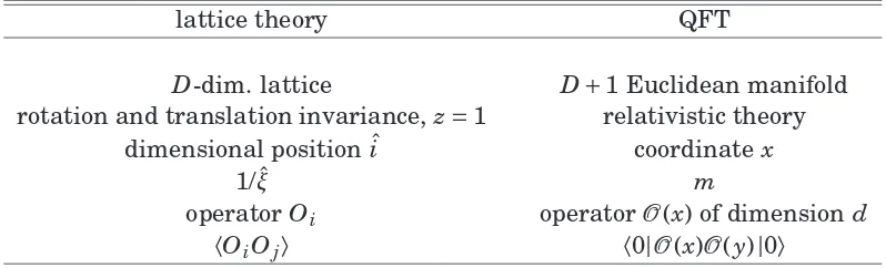
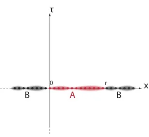
2.1 In this picture we represent a one dimensional lattice system on the real lineT ₌0 which is partitioned into the two regions _Aand

B. Due to translation invariance the region Ais only defined by its

length r, and we choose A_∈[0,r]. The blurred curves around the

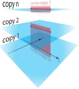
lattice represent the field configurations of the scaling quantum field theory. . . 40 2.2 Representation of the multi-sheeted surface M. Each blue layer

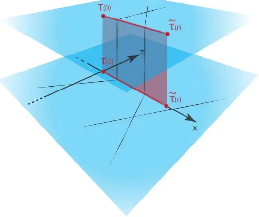
represents a copy of the model at hand, and they are connected through the red branch cut. . . 44 2.3 We show the effect ofT and ˜T on fields configurations. The black

lines can be interpreted as the centre of some wave packets propa-gating in the incrasingτdirection. . . 47

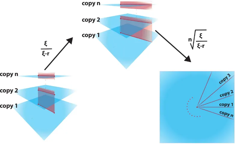
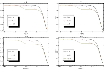
2.4 We show the sequence of transformations which unravel the man-ifoldM onR2. . . 48 3.1 The function ∆(_t) :₌∆_T(_t) with _t₌2log( ˜_r) and ˜_r₌_mr. In these

(13)

con-LIST OF FIGURES

4.1 In this picture we show the difference between ∆(_t), and _c(_t) for two copies of the Ising model (n₌2). We carried out the same

analysis until n₌10, finding the same qualitative behaviour. The

scale is logarithmic, and we can see that, even if at the critical point∆_T(0)₌ c(0)

24

¡

n₋1_n¢, along the RG flow this equality does not

hold anymore. . . 102 4.2 In this picture we are representing the self-interaction

contribu-tions to the stress energy tensor with an arrowed solid line. We chose to place the branch cut on the negative real axis. The dashed line represent those contributions which are forced to loop around other copies to close. . . 108 5.1 phase diagram of the XY spin chain. . . 133 5.2 Energy levels of the scaling Ising chain. . . 137 5.3 Representation of the bipatition in the two regions A, and its

com-plement. The external magnetic field is aligned along the z-axis,

while the black links between spins represent the bond interaction. 140 5.4 Behavior of the entanglement entropy for fixed block length as a

function ofh. . . 146

5.5 Behavior of the entanglement entropy for fixed h as a function of

the block length. . . 147 5.6 Plot of the critical entanglement entropy S(L,1). The numerical

data are shown in red, along with the fitting logarithmic behaviour (5.49) as a blue dashed line. . . 148 5.7 In this figure we plot the numerical data obtained for the

Bessel-like term in eq. (5.52) for different values of the correlation length

ξ. We can observe how even for relatively small ξ the scaling

be-haviourK0(2L_ξ)/8 (black dashed line) fits our numerical data. . . 149

5.8 The numerical values obtained forU₊c′₁ are presented and

com-pared against the analytical prediction in Calabrese et al. [2010]

forS(_∞,ξ)₋1₆logξ, pictured as a dashed black line. The agreement

(14)

LIST OF FIGURES

5.9 The running of the constant αx(ξ) outside the scaling region is

shown for different values ofx. . . 151

5.10 We show data obtained forαx(∞) in the region 1.5≤x≤4,5 with a

numerical fit represented by the black dashed line. . . 152 5.11 Numerical data for the Bessel-like term in eq. (5.76) are compared

with the analytical behaviour represented by the dashed black line. 165 5.12 The numerical results obtained forU₊c′₁ are displayed, and

com-pared with the analytic prediction in Ercolessi et al. [2010]. The

accordance is lower than for the Ising case, but good enough to confirm confidently the analytic behaviour. . . 166 5.13 Numerical estimate of α(ξ) obtained with a best fit of the

Bessel-like term in eq. (5.52). The black dashed line is the best linear fit

(15)

List of Tables

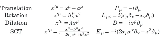
1.1 Summary of the map between a lattice theory and its correspond-ing scalcorrespond-ing quantum field theory. . . 22 2.1 Finite conformal transformations, and generators of the

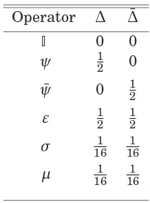
infinitesi-mal transformations in general dimensions. . . 29 3.1 Operator content of the Ising model. σ andµ are usually referred

to as order and disorder operators respectively in light of the cor-respondence with the two-dimensional Ising lattice theory. . . 60 3.2 Two particle contribution to the conformal dimension in the

RT-model. The second column shows the exact values of the conformal dimension of the twist field corresponding to central charge c3=

1/2. The third column shows the numerical values of the same quantity in the two-particle approximation forθ0=20. . . 91

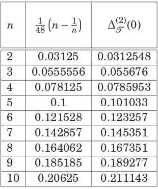
3.3 Four-particle contribution to the conformal dimension in the RT-model. The second column shows the difference between the val-ues of the conformal dimension of the twist field corresponding to central chargesc4=7/10 andc2=1/2. The third column shows the

(16)

LIST OF TABLES

3.4 In this table we display the value ∆T(t) for different n when we

approach the UV limit t_{→ −∞} considering different values of the

resonance parameters σ. We observe a good agreement with the

CFT prediction (2.67) with c₌6/5. . . 95

5.1 Asymptotic behavior for large distance of the correlation functions of the XY chain near the Ising critical lineh₌1. . . 136

5.2 In this table the details of our DMRG simulations are reported.

Ls is the length of the chain, mi the number of states kept in the

infinite phase, mf the number of states kept in the finite phase,

(17)

1

Introduction

The first two decades of the 20th century were characterized by great intellectual ferment in the physics community. The works of J. C. Maxwell on the electromag-netic waves, summarized in his 1873A Treatise on Electricity and Magnetism1,

paved the way to a technological boost which in turn gave access to a new set of experiments. Consequently new problems rose, which were not interpreted by any mathematical theory available to a scientist of that time. A first exam-ple was Maxwell’s incapability of explaining the propagation of electromagnetic waves in the vacuum. The only kind of waves known then were pressure waves, which clearly needed a medium for propagation. This led to the supposition of the existence of a luminiferous aether, that was a fine substance which acted as

a bearer of light.

It was in 1887 that an experiment led by A. Michelson and E. Morley demon-strated the nonexistence of such a substance. The problem of how electromag-netic waves could propagate in the vacuum remained then unsolved, and opened a quest that found its end with the formulation of a theory of relativity, and quan-tum mechanics. In particular it was A. Einstein who first introduced the concept of a light quantum (particle) in his most celebrated work on the photoelectric effect Einstein [1905].

This wave-particle duality helped solving many other difficulties that mathe-matical models had in describing experiments of the time. The most remarkable example was the ultraviolet catastrophe of the black-body radiation. Maxwell’s

(18)

theory describes the energy of the electromagnetic field inside a cavity as an in-tegral over the whole frequency spectrum. This leads to the divergence of the heat capacity, and then to infinite energy at any non-zero temperature. This di-vergence was clearly not observed in experiments. This problem was solved by M. Planck in 1900, when he assumed that the energy distribution were discrete in frequencies, finding a perfect agreement between his prediction and experi-mental results. The discreteness of the spectrum led again to the natural inter-pretation of the radiation as jets of particles, that were calledquanta.

The scientific community started then a thorough investigation of this duality, which finally was embedded in a more comprehensive theory of quantum me-chanics. Two parallel mathematical descriptions of quantum mechanics were born during those years, a matrix mechanics developed by W. Heisenberg, and

a wave mechanics developed by E. Schrödinger. These two apparently distant

formulations were proven equivalent, and unified later by P. M. Dirac. Such theories were based on few shared very solid principles:

1. thewave-particle duality. Not only radiation, but any kind of object can

show particle or wave properties, depending on how it is tested.

2. The uncertainty principle. There are some conjugated couples of

ob-servables which cannot be measured on the same system. This can be rephrased as if the measurement of one observable would lead to errors on the second observable large enough to frustrate any prediction.

3. The quantum essence of nature. Performed at small scales,

measure-ments’ outcomes of any physical quantity can be counted in multiples of a

quantum.

4. The superposition principle. Until a physical quantity is measured, it

does not have a defined value, it is instead in a superposition of all possible outcomes of a supposed forthcoming measurement.

(19)

quan-in the quan-interaction picture. In this language a physical system is described by a vector_|v_〉which lives in a Hilbert spaceH. The superposition principle is natu-rally interpreted in this formalism, as the possibility of representing a state by a linear combination of vectors

|v_{〉 =}X

j

αj

¯

¯aj〉, with αj∈C,

¯

¯aj〉 ∈H,∀j. (1.1)

The coefficientsαj are bounded byPj

¯ ¯αj

¯

¯2₌1, and they are linked to the prob-ability that a measurement on any physical quantity contained in _|v_〉 gives the

value contained in¯¯aj〉. Physical quantities are called observables, and they are

represented by self-adjoint operators O₌O†. The measurement process is

re-sponsible for the collapse of the state in one of the possible eigenstates of the measured observable. Calling Ok the eigenvalues of O, and |ok〉 its

eigenvec-tors we define the expectation value ofOin the physical setting described by the

vector_|v_〉as

〈O_{〉 =}X

k

|〈ok|v〉|2Ok. (1.2)

The interpretation of (1.2) is that a measure ofOgivesOkas a result with

proba-bility_|〈ok|v〉|2. This forces the state|v〉to “align” with the vector|ok〉,

constrain-ing the possible outcomes of followconstrain-ing measurements.

The probabilistic interpretation of a quantum state was unpalatable to A. Ein-stein, who, with B. Podolsky and N. Rosen, collected his doubts in the renowned paper Einsteinet al. [1935]. In their opinion any theory which aims to describe

the physical reality, must be complete1. The first objection to quantum mechan-ics is that if two variables do not commute (e.g. position and momentum of a wave packet) they cannot be measured at the same time, indeed a measurement on one variable which exactly determines its value would constrain the second one to have a flat statistics. Then the second quantity has no physical reality. This means either that the two quantities cannot have both physical reality, or that the theory is not complete. Their conclusion was that if both the quantities have an experimental counterpart the theory must not be complete.

(20)

There is a second example in that paper, which goes a bit deeper on the matter, and opened a long history of debate. It is worth reporting it here in the fashion of the original paper. Suppose we have two quantum system, namely A and B,

which interact together for a finite time t_∈[0,T]. At timeT we divide them, and

we give them to two observers, Alice and Bob, who are spatially separated. The quantum state of the two systems is determined for t_<0, while later on it

be-comes the state of the composite system A_∪B, which has to be determined. The

authors used the Schrödinger wave function formalism to describe the problem, so that the whole system is described by a wave function Ψ(_x). Now suppose that Alice performs a measurement of some observable U. We callu1,u2,... the

eigenvalues of such operator, and u1(xA),u2(xA),... the corresponding

eigenvec-tors, where xAis the set of variables associated to the system A. Then the wave

function can be rewritten as

Ψ(_x_A,_x_B)₌X∞

n=1

ψn(xB)un(xA), (1.3)

and the measurement performed by Alice has the effect of “selecting” one of the

uk(xA) by the outcome of uA, and then projecting Bob’s system onto the state

ψk(xB). Now suppose Alice chooses to measure another quantity V, then we can

write

Ψ(_x_A,_x_B)₌

∞

X

n=1

φn(xB)vn(xA). (1.4)

A measurement of V will project A onto a particular eigenstate vl(xA), and B

onto φl(xB). The conclusion is that two different measures on the system A

would leave the state Bdescribed by two different wave functions. On the other

hand, since there is no more physical interaction between AandB, an action on

one of the two sub-systems should not influence the state of the other. In their work the authors were using this feature to demonstrate the non-completeness of quantum mechanics, but this goes beyond the scope of this introduction, and we will take for granted their point of view.

(21)

managed to describe how the existence of local hidden variables influences the statistical correlations of a model by a set of inequalities, and finally showed that quantum mechanics violates those inequalities. By doing so he demonstrated that quantum mechanics is not a local hidden variables theory, and that its cor-relations cannot be reproduced by classical corcor-relations.

We need to wait until the works of Freedman & Clauser [1972] and Aspectet al.

[1981, 1982] to have the first convincing experimental realizations of the vio-lation of Bell’s inequalities. In the meantime the scientific community started identifying this long range effect typical of a quantum system under the name ofquantum entanglement. In the following section we aim to formally define

this phenomenon.

1.1 Quantum entanglement

Entanglement is probably the deepest (certainly the most obscure) manifesta-tion of the quantum approach to reality. It finds its origin in the superposimanifesta-tion principle when one is dealing with a composite system. The classical description of the dynamics of a many-body problem is performed in the phase space, whose dimension grows linearly with the number of components1_{. In a quantum}

me-chanical description the corresponding concept is the Hilbert space H, which is a tensor product of its componentsH ₌NN

i=1Hi, such that its dimension grows

exponentially with the number thereof.

We will take the Hilbert spaces of each component to have the same dimension

d, then a global state is represented as the vector

|Ψ_{〉 =}

dN

X

{ι}

aι

¯

¯ψι〉, (1.5)

where ιis a N-tuple, and it is summed over all its possible configurations, that

aredN. The vector part of each term can be decomposed on the complete basis of

(22)

the subsystems¯¯uk_〉in the following way

¯ ¯ψι〉 =

¯ ¯

¯u1_i₁_{〉 ⊗}¯¯_¯u2_i₂_{〉 ⊗}..._⊗¯¯_¯uN_i

N〉, with 1≤ik≤d,∀ik∈ι. (1.6)

In order to ease the notation we will use the two components case in our forth-coming definitions, and will refer to it as a bipartite system. Unless stated dif-ferently all the considerations we make can be extended trivially to the generic

Ncase. In the case of two subsystems eq. (1.5) can be written as

|Ψ_{〉 =}

d

X

i,j=1

ai j

¯

¯u1_i_{〉 ⊗}¯¯_¯u2_j_〉. (1.7)

Here two cases must be distinguished:

1. the coefficients ai j can be factorized into products, e.g. ai j =αiαj. The

state can be rewritten then as

|Ψ_{〉 =}

Ã

d

X

i₌1

αi

¯ ¯u1_i_〉

!

⊗

Ã

dN

X

j₌1

αj

¯ ¯ ¯u2_j_〉

!

, (1.8)

and it is calledseparable, orfactorizable.

2. The coefficientsai j cannot be factorized, and the state is calledentangled.

The case in which the two subsystems’ Hilbert spaces have different dimensions needs extra care. This case can be treated using the Schmidt decomposition Schmidt [1907]. Suppose the two systems have dimensionsmandnwithm_<n.

Then considering the state (1.7) the coefficientsai j can be written as the entries

of an m_×n rectangular matrix A. This in turn can be written as A₌UλV†,

whereUis an m_×m, andVan n_×nunitary matrix, whileλis an m_×n matrix

with null off-diagonal entries, and a numberrof non-zero real diagonal elements

λ1≥λ2≥...≥λr. The number of non-zero eigenvaluesr is usually referred to as

rank, and it is a property shared by the two subsystems.

(23)

rank1

¯ ¯ψ_{〉 =}

r

X

i=1

λi

¯

¯u1_i_〉¯¯u2_i_〉

¯ ¯φ_{〉 =}

r

X

j=1

ηj

¯ ¯ ¯v1_j_〉

¯ ¯ ¯v2_j_〉.

(1.9)

It can be demonstrated that¯¯ψ_〉 can be transformed into¯¯φ_〉 by local operations

and classical communication (LOCC) iff

k

X

i=1

λi≤ k

X

j=1

ηj, ∀k∈[1,r]. (1.10)

This is calledmajorization rule.

1.2 The density matrix

States of the kind (1.6) are usually calledpure states. There exist a second class

of states which are referred to asmixed states, and they are described by a

sta-tistical ensemble of pure states. The stasta-tistical distribution can be for example canonical, and induced by considering a thermal state. The standard way to tackle this situations is by introducing thedensity matrix

ρ₌X

i₌1

pi

¯

¯ψi〉〈ψi

¯

¯, (1.11)

where pi are the probabilities associated to the states

¯

¯ψi〉 with the

aforemen-tioned distribution2. This matrix is positive definite, and of trace 1, and the expectation value of any observableOcan be defined as_〈O_{〉 =}Tr£ρO¤.

In parallel with the definitions in section 1.1, Werner [1989] defined as separable

1_{from now on we will drop the tensor product symbol between Hilbert spaces for convenience,} such that_|a_{〉 ⊗ |}b_〉will be abbreviated_|a_〉|b_〉.

2_{in the example of a quantum state in equilibrium with a thermal bath} _p

i=e−

E i

kT, where we are considering the case where¯¯ψ_i_〉are eigenstates of the Hamiltonian, with eigenvaluesEi,

(24)

those mixed states that can be written as

ρ₌X

i=1

piρi₁⊗ρ₂i, (1.12)

and called entangled those states which cannot.

A very interesting and well understood setting in which entanglement can be studied is that of a bipartite pure system. Suppose we have a global system described by the pure state ¯¯ψ_〉, which we bipartite into two subsystems A and B (a setting which is totally analogue to the one of Einsteinet al. [1935]). The

density matrix associated to this global state contains clearly just the state ¯¯ψ_〉,

with probability pψ=1, that isρAB=

¯

¯ψ_〉〈ψ¯¯. The question we want to answer

is: Given the knowledge of ρAB can we make predictions for the outcomes of a

measurement on A or B?

It is generally impossible to associate a pure state to one of the two subsystems, but if we want to study the properties of say A, we can trace out the system B.

In detail this means first choosing a complete basis of B, which we call_|bi〉, and

then acting on the global density matrix with the projectors on this basis in the following way

ρA=

X

i

〈bi|ρAB|bi〉. (1.13)

The reader may be confused by the notation adopted in eq. (1.13). In the rhs of eq. (1.13) we are performing a partial trace on the subsystemBof the whole

sys-tem A_∪Bon whichρAB has support. As a result the outcome of such a trace is

not a scalar, but rather a matrix, which we callreduced density matrixof the

sys-temA. If there is entanglement between the two subsystems this will be a mixed

state’s density matrix. This is equivalent to admitting total ignorance about the system B, hence associating equal probability to the outcomes of any

measure-ment of an observable with support on B. This process is usually referred to

as “tracing out” the region B, such that an equivalent notation for eq. (1.13) is

ρA=TrBρAB.

(25)

are two electrons, and their spin wave function is in the singlet state

¯

¯ψ_〉_AB₌_p1

2(|↑〉A|↓〉B− |↓〉A|↑〉B), (1.14) where_|↑〉and_|↓〉are the two spin eigenstates along the z-axis1_{. It is easy to check}

that the two electrons are entangled in this case, as with simple calculations one manages to expressρA=1₂(|↑〉A〈↑|A+ |↓〉A〈↓|A).

Now that we have a way to distinguish two entangled bipartitions from non-entangled ones we aim to define a way of quantifying entanglement.

1.3 Entanglement measures

In order to define an entanglement measure it is helpful to think about the con-cept of reduced density matrix (1.13). That matrix is used to define the expecta-tion values of any operators acting on the subsystem A. The more these

expec-tation values are correlated with those on B, the more the two subsystems are

entangled, the more ρA will be mixed2. As a consequence the more this matrix

is mixed the more we have access to information about B, and possibilities to

influence the outcomes of measures of its observables3.

Another very important aspect of entanglement is its relationship with informa-tion. Referring to the usual example of the bipartite system if the bipartitions are entangled, somehow their density matrices capture more information about the state thanρAB. This feature, even if already noticed by Schrödinger in the

Thirties, was put on a solid basis and quantified in Schumacher [1995]. In this latter work a quantity called entanglement entropy was defined, which extends

the concept of the Shannon entropy of a statistical distribution to the quantum

1_{this example actually works with any binary systems.}

2_{there is no measure of how mixed a density matrix is, more mixed means that its eigenvalues} are closer to being all equal.

(26)

case, and is defined as1

S(ρ)_{= −}Trρlogρ. (1.15)

The entanglement entropy as defined here is usually calledvon Neumann entan-glement entropy, and has the following interesting properties:

• It is null for separable states and maximal in the case in which the density matrixρhas all nonzero equal eigenvalues. In that case, due to the

normal-ization ofρ, if the Hilbert space isd-dimensional, we will haveS(ρ)₌logd.

States of the kind defined in eq. (1.14) are the easiest examples, and they are calledmaximally entangledstates.

• If ρAB is the density matrix of a pure state, S(ρA)=S(ρB). This can be

shown trivially by Schmidt decomposing the state, and has remarkable implications explained in section 1.7.

• It is invariant under unitary transformations of the density matrixU†ρU,

and then independent of the basis in which it is expressed.

• It is concave, in the sense that for a mixed state P_ipiρi the property

P

ipiS(ρi)≤S(Pipiρi) holds.

• It has the remarkable propertyS(ρAB)≤S(ρA)+S(ρB). This property does

not have a counterpart in classical information theory, where the entropy of a system can never be lower than that of its components, and is called

subadditivity. A more general version of this property can be written if one

considers the possibility of an intersection between the two subsystems A

and B, where the subadditivity states that S(ρA∪B)+S(ρA∩B)≤S(ρA)+

S(ρB).

The entanglement entropy (1.15) plays a central role in determining how many singlet states can be distilled from a general mixed state, outlining an operative definition of it2_{. Before walking this way though we have to consider}

(27)

if a general state is transformable at all, and to which states. The answer comes from the majorization rule (1.10), which tells us which states are compatible, and which are not. A problem in this approach is the presence of discontinuities in the probability of transformation from one state to the other. To make this statement clearer we borrow an example from Plenio & Virmani [2007]. Let us consider the composition of two ternary states, such that the Hilbert spaces of each component are spanned by the basis {_|0_〉,_|1_〉,_|2_〉}. It is easy to check with (1.10) that the state (_|00_〉+|11_〉)/p2 can be transformed into 0.8_|00_〉+0.6_|11_〉. That means there exists a local transformation which links the two states with probability equal unity. If we introduce a deformationεleading to (0.8_|00_〉+0.6_|11_〉+ε_|22_〉)/p1₊ε2, we can

check that this state cannot be reached for any nonzero value of ε. This can be

easily understood by considering that LOCC cannot increase the rank of a state. This feature is somehow unwanted, as the expectation values of any physical quantity will depend on ε, and we do not expect discontinuities varying such a

parameter.

This problem can be tackled by considering a less ideal setting. Instead of ask-ing if two states are compatible we can ask if a set of n identical states can be

transformed into a set of m states, “close enough” to a target state, that is a

de-formationεof a target state which tends asymptotically to it for large n andm.

Formally calling ρ the density matrix of an initial state, andσ that of a target

state, we want to see if it is possible to transform n copies ofρ,Nn_i₌₁ρi→σm(ε),

where σm(ε)→Nm_i₌₁σi for m→ ∞. An important question is then which is the

biggest rate r₌m/n at which we can perform this transformation?

In particular we would like to define the entanglement cost EC(ρ) as the rate

at which we can convert a set of n maximally entangled binary states as (1.14)

(whose density matrix we call ρ) into a set of mtarget states σ. So that calling

Λthe LOCC that mapsNn

i₌1ρi→σn(ε)

EC(σ)=MIN

"

r

¯ ¯

¯ _nlim

→∞D

Ã

Λ

Ã _n O

i=1

ρi

!

,Orn

i=1

σi

!

=0

#

(1.16)

where D(ρ,σ)₌p2(1₋F(ρ,σ)) is the Bures distance, F(ρ,σ)₌Trq£pρσpρ¤ is

(28)

is the minimum number of maximally entangled states that we have to employ to “build” a set ofntarget states. We can invert the definition and ask ourselves

how many maximally entangled statesρwe can get out ofnidentically prepared

noisy singletsσ. This leads to the definition of theentanglement of distillation.

This time we define the LOCC which performs the mapΛ(Nn

i=1σi)→ρn(ε)

ED(σ)=MAX

"

r

¯ ¯

¯ _nlim

→∞D

Ã

Λ

Ã

n

O

i=1

σi

!

,Orn

i=1

ρi

!

=0

#

. (1.17)

The entanglement cost, and entanglement of distillation are of central relevance when dealing with experimental realizations of quantum protocols. In fact in the real world preparing a binary system in a maximally entangled state is gener-ally a difficult task. Moreover, as those protocols are based on the transmission of a quantum state, one has to deal with decoherence due to noisy channels. Quantum information is mediated by qubits, extracted from maximally entan-gled states, hence understanding how to optimize the conversion of a noisy state into a maximally entangled one is very important.

It was demonstrated by Bennettet al.[1996] that for pure statesEC(σ)=ED(σ),

so that the process is asymptotically reversible. Most remarkably they are both equal to the Von Neumann entropy, which in this case is the only relevant mea-sure of entanglement.

Other measures of entanglement are theRényi entropies, introduced in their

classical version by Rényi [1961]. These quantities are dependent on a real pa-rameterα_≥1, and are defined as

Sα(ρ)= 1

1₋αlogTrρ

α_. _(1.18)

They clearly have the Von Neumann entropy as the limit for α_→1. To

under-stand their utility we have to diagonalize the density matrixρ, such that

Sα(ρ)= 1 1₋αlog

Ã

d

X

i=1

λα_i !

(29)

where d is again the dimension of the Hilbert space. AsPd_i

=1λi=1, the sum in

eq. (1.17) converges for any value of α_∈[1,_∞), andSα(ρ) is well defined. More-over considering large values ofαsuppresses the lowest eigenvalues ofρ(lowest

levels in the entanglement spectrum 1_{), while small values of}_α _{take them into}

account. From these considerations follows that the knowledge of the Rényi en-tropies for general αgives access to information about the whole entanglement

spectrum. In particular now we have a way to understand the majorization rule in eq. (1.10). It is telling us that LOCC cannot increase the entanglement be-tween the two components, in the sense that Sα(ρφ)≤Sα(ρψ), for anyα.

Another interesting question one can ask is: Considering a single copy of a generic state, which is the dimension of a maximally entangled state distilled with

certainty?

The answer is given by the single-copy entanglement as defined by Eisert &

Cramer [2005]. Suppose that the a density matrixρcan be transformed by LOCC

into ¯¯ψD〉〈ψD

¯

¯, where ¯¯ψD〉 =

¡

|α1〉¯¯β1〉 + |α2〉¯¯β2〉 +...+ |αD〉

¯ ¯βD〉

¢

/pD, then we

define its single-copy entropy as E1(ρ)₌logD2.

For this transformation to be possible condition (1.10) must be satisfied, then calling againλi the eigenvalues ofρ, and ordering them as decreasing withi, we

have

k

X

i=1

λi≤

k

D, ∀k∈[1,D]. (1.20)

This naturally impliesλ1≤1/D. We can then express the single-copy

entangle-ment in terms of the original density matrix eigenvalues as

E1(ρ)=log¡⌊λ−11⌋¢, (1.21)

1_{we use the notion of entanglement spectrum as introduced by Li & Haldane [2008], and}

Calabrese & Lefevre [2008].

2_{the reader may be surprised by the fact that we are talking here about a}_D_-dimensional

(30)

where with_⌊..._⌋we are taking the integer part. In particular, exploiting the fact that logTrρα_∼αlogλ1 for α→ ∞, we can link the single copy entanglement to

Rényi entropies

E1(ρ)= lim

α→∞Sα(ρ). (1.22)

1.4 Quantum entanglement and many-body

sys-tems

One of the most intriguing challenges in modern physics is the description of quantum many-body systems. In particular in recent years a great deal of atten-tion has been given to the connecatten-tions with quantum informaatten-tion theory. Indeed many open problems in many-body physics have been successfully treated with quantum information techniques. On the other hand many new protocols in quantum computing have been inspired by many-body problems, as a quantum processor is itself a many-body system.

Quantum mechanics is very effective in studying single-body problems, or sys-tems composed of few constituents. As we increase the number of components though, systems become rapidly intractable due to the exponential growth of the Hilbert space explained in section 1.1.

A real system is seldom composed by few components, hence quantum mechan-ics would seem powerless in predicting any outcomes of an experiment. For-tunately in a great deal of cases interactions between components are fairly small compared to the energy scale of each constituent. Therefore the prob-lem can be treated perturbatively using single-body techniques. Many cases though cannot be treated as such as they are characterized by strong interac-tions. Among them there are some very relevant problems in modern physics, such as bosonic condensates, strongly correlated electrons, studied in the quest for high-temperature superconductivity, and last but not least the physical real-ization of a quantum computer.

(31)

be-Hilbert space quickly grows too large to be implemented even on the most re-cent machines. Then it becomes very important to understand when a quantum system can be simulated efficiently on a classical computer1_{. The answer was}

given indirectly by White [1992], and it was cast in a quantum information per-spective. The system’s components must be weakly entangled more than weakly interacting, in order to succeed with a numerical simulation. This observation gave rise to a set of very powerful numerical techniques which go under the name

ofdensity matrix renormalization group(DMRG).

There are many other examples of cases in which the study of entanglement properties of a many-body system leads to new insights. One of the most re-markable is the existence of quantum phase transitions (QPT). The remaining

part of this section is devoted to explaining qualitatively the main features of QPT. For a more detailed analysis we redirect readers to Sachdev [2007]. We fo-cus on the zero temperature case, so that any phase transition will be driven only by quantum effects, and the system will be in a pure state rather than a thermal ensemble. We take the system to be in its ground state. To help the understand-ing we focus on a quantum magnet as an example. The degrees of freedom are concentrated in the magnetic cells, which, with a drastic simplification, can be represented by sites with a spin degree of freedom. The interaction among them can be represented by a link on a lattice. Here and throughout this manuscript we will consider only the case of nearest neighbours interactions. The cells can be coupled to an external magnetic field by their spin magnetic momentµh.

Sum-marizing all these considerations we can write the general Hamiltonian of this system as

H(_J,_h)₌_J X

〈i,j〉

~

Si~Sj−gµhh

X

i

~

Si~ui, (1.23)

where _S~

=~_σ/2, _J sets the microscopic energy scale of the interaction between sites, g is the g-factor (_≃2 for electrons),h is the intensity of the magnetic field,

and~_u is a versor pointing in the direction of the external field. Notice that al-though eq. (1.23) is independent of the lattice spacing a and the lattice shape,

the physics will depend to a great extent on these quantities.

The Hamiltonian (1.23) is a representative of a family of systems which can be

(32)

written asH(_h)₌H₀₊_hH₁,_hbeing a dimensionless parameter. For any fixed value ofhwe can diagonalize the Hamiltonian, and find the energy levelsEi(h),

and the respective eigenstates¯¯ψi(h)〉. We focus on the case in whichH1is a

con-served quantity, that is, it commutes withH₀1. This means that the eigenvectors do not depend on h, as for any value of this parameter they are the eigenstates

of H₀. The energy levels on the other hand are smooth functions of _h. We fo-cus then on the ground state energy E0(h), and we want to study its behaviour.

It can happen that for a given h₌hc, the eigenvalue of an excited state equals

E0(hc), then we have a point of non-analyticity of the ground state energy2. We

call these points quantum critical points, and they usually separate two regions in which the system shows very different responses to an external perturbation. In particular we focus on second order QPT which are characterized by collective phenomena which in turn give rise to long-range correlations. This features can be formalized considering the model (1.23) in the case of an infinite, traslational-invariant lattice. We can define the correlation between spin components along e.g. thez-axis as

〈Sz_iSz_j_{〉 = 〈}ψ0(h)¯¯SziS z j

¯

¯ψ0(h)〉 − 〈ψ0(h)¯¯Szi

¯

¯ψ0(h)〉〈ψ0(h)¯¯Szj

¯

¯ψ0(h)〉. (1.24)

It is generally a hard task, but it can be demonstrated that the large distance limit of this quantity is exponentially suppressed as

〈S_izSz_j_{〉 ∼}e−| i−j|

ξ(h) ₍₁₊Σ_d_), (1.25) where ξ(h) is called correlation length3. The quantity Σ_d is a sum of infinitely many terms having a more suppressed exponential behaviour. There are some integrable theories for which it is possible to sum this series finding a power law.

1_{notice that this is not usually the case, but we assume this in order to be able to explain the} main features of a QPT in a compact and direct fashion.

2_{to be precise this feature, called}_{level crossing}_{, is possible only when}_H

1 is a conserved quantity. In the most general case the two energy levels only come very close, but do not meet, and this feature is calledavoided level crossing. In certain limits though many of these avoided level crossings become level crossings, so that our arguments are of wide applicability.

(33)

dimen-In a second order phase transition we have ξ(hc)= ∞ and it is actually much

easier to sumΣ_d. The correlation function will be described by a power law

〈Sz_iSz_j_{〉 ∼ |}i₋j_|−2d, (1.26)

allowing for long-range interactions. The constant dis usually calledscaling di-mension.

The correlation length is then again an analytic function of h, except at the

crit-ical point, and it is particularly interesting to study its behaviour approaching

hc. For the model at hand, it diverges with the power law

ξ(h)_{∼ |}h₋hc|ν, (1.27)

whereνis calledcritical exponent.

Another interesting feature is the collapse of the first excited state onto the ground state. This means that if we define theenergy gapas∆(_h)₌_E₁(_h)₋_E₀(_h) we have ∆(_h_c)₌0. The way this quantity approaches zero, and the correlation length diverges are related by

∆(_h)_{∼ |}_h₋_h_c_|zν, (1.28)

which means that∆_∼_ξ−z. The exponent_zis usually called_{dynamical exponent}. To elucidate this relation we consider the model (1.23) on a D-dimensional

infi-nite lattice as an example. In what follows is crucial that the lattice is invariant under rotations, that is under exchange of two axes and respective coupling con-stants.

The Hamiltonian describes the temporal evolution of the system, and we per-form a Wick rotation so that we work with imaginary time τ. Then for τ small

enough we can define the transfer matrixT₌1₋τH _≃_e−Hτ. We take a discrete time that we count in terms of the lattice spacing a, which we set to be equal

one for simplicity. Then we can study this problem as a statistical model on a

D₊1-dimensional lattice, where the wave function at two consecutive times will

be connected by the transfer matrix ¯¯ψ(τ₊1)_{〉 =}T¯¯ψ(τ)_〉. Due to the invariance

(34)

subspace in any D dimensions, evolving in the orthogonal dimension. We want

to study the same site, different times correlation function, that is _〈Sz_i(0)Sz_i(τ)_〉.

We represent our operators in the Heisenberg picture, such that

〈S_iz(0)S_iz(τ)_{〉 = 〈}ψ0¯¯Sz_i(0)e−HτSz_i(0)eHτ¯¯ψ0〉 − 〈ψ0¯¯S_iz(0)¯¯ψ0〉〈ψ0¯¯Sz_i(0)¯¯ψ0〉 =

= X

k≥1

¯

¯_〈ψ0¯¯S_iz(0)¯¯ψk〉

¯

¯2e−(Ek−E0)τ_,

(1.29)

where we have assumed the theory has a discrete set of eigenvalues1_{. The first}

gap is usually much wider than the others, and we can rewrite the latter in terms of it asEk+1−Ek=αk∆, wherek≥1, and 0<αk<1.

We can then rewrite (1.29) as

〈Sz_i(0)Sz_i(τ)_{〉 =}¯¯_〈ψ0¯¯Szi(0)

¯

¯ψ1〉¯¯2e−∆τ

Ã

1₊X

k_>1

δke−αk

∆_τ

!

, (1.30)

where δk=

¯

¯_〈ψ0¯¯Sz_i(0)¯¯ψk〉/〈ψ0

¯

¯Sz_i(0)¯¯ψ1〉¯¯2 . Is now easy to compute the

expo-nentially decaying behaviour in the limitτ_{→ ∞}in the off-critical case, where∆ has a fixed value. The series in the rhs of eq. (1.30) is generally very hard to sum, and one has to consider the fact that the spectrum is not entirely discrete. Rotation invariance gives us the correspondence ξ_∝1/∆, and a direct compari-son with eq. (1.26) tells us that the dynamical exponentz₌1, as usual for second

order phase transitions. This will generally be the case for the theories studied in this manuscript.

1.5 Generalities on relativistic quantum field

the-ory

(35)

rela-tivistic QFT.

One of the main goals of a QFT is the study of correlation functions of local fields, as they are the only physical quantities in the theory, in the sense that they can be related to observables. First we want to settle what we mean by locality. In a relativistic theory we say that a field is local if it is causally independent of any other fields for space-like intervals. We apply this definition on a countable set of fieldsφa(x)a∈N. This is a set of local fields if

£

φa(x),φb(y)

¤

=0 ∀a,b_∈N _∀_x,_y

¯ ¯

¯ ¡x0₋y0¢2_{< |}~_x₋~_y_|2 (1.31) This definition is quite cumbersome as it is, and can be simplified further. In fact the temporal evolution of a field is governed by the HamiltonianH ₌R_dxD_h(_x), where h(x) is the energy density. We can define locality by asking that h(x) do

not depend on any other fields for space-like intervals, that is

[φa(x),h(y)]=0 a∈N ∀x,y

¯ ¯

¯ ¡x0₋y0¢2_{< |}~_x₋~_y_|2 (1.32) If we prepare a configuration of fields which satisfy eq. (1.32) we can easily see that any later configuration will automatically satisfy eq. (1.31), so that the two definitions are equivalent. This is due to the fact that due to eq. (1.32) any later couple of fields will be quantum mechanically independent, and then eq. (1.31) holds.

As we will see in the next section the real equivalence is between quantum lattice theories close to criticality, and Euclidean QFT. The next step is then to define the correlation functions in the Euclidean QFT as

〈0|φa1(x1)φa2(x2)...φan(xn)|0〉 =

1

Z

Z_£

D_φ¤_φ_a

1(x1)φa2(x2)...φan(xn)e−

S[φ]_{, (1.33)} where S[φ] is the action functional, and Z₌R£D_φ¤_e−S[φ] the partition function. The connections of this expression with a lattice theory, and in particular of the integration measure, will be explained in section 1.6.

(36)

linearly as

O(_x)₌ X

n∈N

anφn(x), (1.34)

where an are c-numbers. Here we are simplifying heavily the notation and we

are not expressing explicitly any quantum number, but clearly all quantum num-bers of the lhs and the rhs must match. Examples of such a set are the ordered products of powers of the field and its derivatives for a free bosonic theory. Equa-tion (1.34) has to be taken in the weak sense, viz. is true only when the operator O appears into an expectation value.

Another remarkable feature of a relativistic QFT is the existence of anoperator product expansion. Consider a physical process which is characterized by two

op-eratorsO₁(_x₁) andO₂(_x₂) separated by a very small distance1 compared with all the other operatorsϕi(yi) taking part in the process. It is sensible to think that

fluctuations of these two operators are not felt by ϕi, so that their product can

be replaced by an effective vertex in the diagrams contributing to the process. Following this idea we can then state

O₁(_x₁)O₂(_x₂)₌ X

n_∈N

cn₁₂(_|x1−x2|)φn(x1), (1.35)

where cn₁₂ are c-number functions, dependent only on the nature and relative

positions of the operatorsO₁(_x₁) andO₂(_x₂). Again as in eq. (1.34) the only fields allowed in the rhs are those with quantum numbers compatible with the lhs.

1.6 Quantum field theory as scaling limit

(37)

ask ourselves if a quantum field theory can be used even outside criticality. The answer to this question is yes, but in a very particular case.

The idea comes from the fact that if we are “close enough” to the critical point the physics is described by low energy excitations. This can be seen with (1.28), that is in the region where ξ is very large, the gap is almost null, and energy

levels are shifted towards the ground state. This means that the wave function’s spectral decomposition is governed by low energy modes, whose oscillations are very big compared to the lattice spacing. Describing the low energy physics of the model means looking at large distance, and looking at larger distance is in turn equivalent to reducing the lattice spacing. The equivalence we are after is then between the low energy physics of a quantum lattice model, and a quantum field theory.

We want then to consider a vanishing lattice spacing, but the “naive” limita_→0

changes sharply the physics, as all dimensional physical quantities are mea-sured in lattice spacings. In order to maintain the same physics we have to keep the characteristic length unmodified, and this is achieved by increasing ξ. This

means taking the limit a_→0, and the limit ξ_{→ ∞}. Loosely speaking we are

reducing the lattice spacing, but at the same time we are zooming into the sys-tem, in such a way that we observe the same characteristic distance. In a more physical fashion it means changing the couplinghin the following way

lim

h→hc

lim

a→0[aξ(h)]=

ˆ

ξ, (1.36)

such that ˆξ does not change. The definition of the characteristic length ˆξ is

ar-bitrary, and is this definition which defines the way the two limits in the lhs of eq. (1.36) must be performed. In fact these limits are taken to keep ˆξconstant.

Along with the correlation length, all the lengths have to be rescaled accordingly. That is we want to keep the coordinate of the site ˆi₌ai untouched, and this

means performing the limit i_{→ ∞}. Performing these two limits we can observe

that_〈OiOj〉vanishes asa2d→0. We regularize the correlator by a multiplicative

renormalization. Defining the quantitym₌1/ ˆξwe compute

lim

h→h alim→0

h

(mξ)2d_〈OiOj〉

i

(38)

Under these limits then the correlation function can be rewritten as a two point function of an Euclidean QFT where we called O the quantum field counterpart of the lattice operatorO, and we identified the continuum coordinatesx,y₌iˆ, ˆj.

This relation explains better the meaning of eq. (1.33) in light of the lattice model. In particular allows us to define the integration measure in QFT as

Z_£

D_φ¤₌lim

a→0

" X

config

Y

n_∈N

Y

x

dφ˜n( ˆx)

#

, (1.38)

where ˜φn are the lattice counterparts of fields, and we are summing over all

the possible configurations. This quantity is generally divergent, but a rigorous definition would be far too detailed for our scope.

This sequence of limits is called the scaling limit, and the resulting QFT will

be denoted as scaling theory. A first consequence of eq. (1.37) is that the mass scale of the QFT m is equivalent to the lattice quantity 1/ ˆξ. In particular as it

corresponds to the dimensionful gap ˆ∆ in a relativistic theory, we can interpret this quantity as the mass of the lightest particle in the spectrum. A summary of all the relationships between QFT and lattice quantities is reported in table 1.1.

lattice theory QFT

D-dim. lattice D₊1 Euclidean manifold

rotation and translation invariance, z₌1 relativistic theory

dimensional position ˆi coordinatex

1/ ˆξ m

operatorOi operatorO(x) of dimensiond

[image:38.595.109.508.461.582.2]

〈OiOj〉 〈0|O(x)O(y)|0〉

Table 1.1: Summary of the map between a lattice theory and its corresponding scaling quantum field theory.

(39)

plained in the introduction of Montvay & Münster [1994], in QFT we regularize by discretizing continuum theory, that is introducing a lattice spacinga. In that

case there are ultra-violet divergences that come from the integration over mo-menta of the loop’s contributions. When the QFT is discretized on a lattice, due to the periodicity 2π/aof the Fourier series on the lattice, we can integrate only

over the first Brillouin zone₋π/a_≤p_≤π/a. This clearly gives a finite result, and

the next step would be sending the lattice spacing to zero, and renormalize the theory, exactly as we did in this section.

1.7 The area law

Now that we have a clearer picture on what is and how to quantify entanglement, we can ask ourselves which are the differences between a quantum system and a classical system. An attempt to answer this question is based on the comparison between the classical entropy and the von Neumann entropy.

The first difference is the very interpretation of these two quantities. Entropy enters the classical picture in thermodynamics, where it quantifies the “igno-rance” of a macroscopic observer on the microscopic state of a system. The easi-est example one could think about is an isolated system of fixed energy, volume, and number of constituents. CallingΩthe number of microscopic configurations compatible with the values of macroscopical quantities the entropy isS₌klogΩ. The entropy then quantifies the uncertainty we have on the microscopic configu-ration of the system.

We can make a second more complicated example which is more directly compa-rable with the bipartite setting. Suppose we have a classical many-body system at fixed temperature, volume and number of constituents, and we divide it in a region A and a sorrounding environmentB. We take the last to be big enough

to be considered an infinite energy thermal bath. We allow the two partitions to exchange only heat, and we wait long enough for the two parts to be in ther-mal equilibrium. If we focus on the system A it is sensible to suppose that the

(40)

real number. With a bit of work one can demonstrate that pi=e−

E i

kT holds1, and

the entropy, as defined in thermodynamics, corresponds toS_{= −}kPipilogpi. If

we fix a temperature we can compute the energy _〈E_〉, and the entropy will be S_{= −}k_〈logΩ(_E)_〉. The same statement applies then here, the entropy is again a function of the uncertainty we have on the microscopic configurations. Clearly at zero temperature, where only the lowest energy state is accessible, the two cases are equivalent.

In the quantum case we could have a non-zero entropy even with absolute cer-tainty on the microstate. This can be easily seen with the example of the bi-partite system. If we prepare a classical system in a given microstate, and we bipartite it both the entropies of its partitions are zero. This follows from the fact that we know the global state, so that we know with certainty the microstate of any of its partitions. In the quantum case, as we have seen in section 1.2 this is not true. Even if we prepare the global state with absolute certainty its par-titions can in general have a non-zero entropy. This difference is encoded in the subadditivity property of the entanglement entropy. In the classical case

S(ρAB)=S(ρA)+S(ρB), showing that the two partitions are uncorrelated, while

in the quantum case there is an inequality, showing that there are some left-over correlations between the parties, even at zero temperature.

We want to show an example in which these correlations are well quantified in terms of quantum information. We focus on the bipartite setting, and we calldA

and dB the dimensions of the Hilbert space of regions A andB respectively. An

interesting question is the following: if the global state were a random pure state, what would the average entropy of the region A be?

The answer was conjectured by Page [1993], and proven by Foong & Kanno [1994] and Sen [1996] to be

〈SA〉 ≃logdA−

dA

2dB

(1.39)

1_{this case is an example of a canonical ensemble, and its probability distribution is usually} normalized by a partition function Z. For simplicity of notation here we are assuming Z₌1, which is equivalent to dividing Ω(Ei) by the total number of possible microstates, such that

P