D
EPARTMENT OF
E
CONOMICS
U
NIVERSITY OF
S
TRATHCLYDE
G
LASGOW
CONTESTS WITH GENERAL PREFERENCES
B
Y
ALEX DICKSON, IAN A MACKENZIE AND PETROS SEKERIS
N
O
16-08
S
TRATHCLYDE
Contests with general preferences
Alex Dickson†, Ian A. MacKenzie‡, and Petros Sekeris§
†Department of Economics, University of Strathclyde, Glasgow, UK, G4 0QU. E-mail:
‡School of Economics, University of Queensland, Brisbane, Australia, 4072. E-mail:
§Department of Economics & Finance, University of Portsmouth, Portsmouth, UK.
E-mail: [email protected]
June 13, 2016
Abstract
This article investigates contests when heterogeneous players compete to obtain a share of a prize. We prove the existence and uniqueness of the Nash equilibrium when players have general preference structures. Our results show that many of the standard conclu-sions obtained in the analysis of contests—such as aggregate effort increasing in the size of the prize and the dissipation ratio invariant to the size of the prize—may no longer hold under a general preference setting. We derive the key conditions on preferences, which involve the rate of change of the marginal rate of substitution between a player’s share of the prize and their effort within the contest, under which these counter-intuitive results may hold. Our approach is able to nest conventional contest analysis—the study of (quasi-)linear preferences—as well as allowing for a much broader class of utility functions, which include both separable and non-separable utility structures.
Keywords: contest; general preferences; aggregative game.
JEL Classification: C72, D72
1
Introduction
Contests can be characterized by players expending sunk effort in order to obtain a prize. As this is a rather general economic phenomenon, contest theory has become a dominant framework to explain the incentive structures within a variety of applications, including— but not limited to—rent seeking, patent races, litigation, and conflict (Konrad, 2009). There are two key types of contest studied in the literature: those in which an indivisible prize is contested; and those in which a perfectly divisible prize is shared among contestants. With non-linear payoffs the two are not equivalent, and while the former has been well-studied, the latter has seen much less attention. Although there is large applicability of contests in which a perfectly divisible prize is shared among contestants, there remains a convention within the analysis of such contests to assume players have (quasi-)linear preferences. With such a variety of potential applications at hand, it is, however, perfectly plausible to envisage players with alternative preference structures. Thus the question arises as to whether a tractable analysis of contests with more general preference structures can be undertaken.
general—restrictions on players’ utility functions (such as utility increasing in prize share and decreasing in effort) and can therefore analyze a broad class of potential contest applications. Within such a setting, we show a fundamental component is the rate of change of the marginal rate of substitution between players’ prize share and their contest effort as the size of their share of the prize changes. In particular, we find that this, which is always monotonically decreasing in the standard contest model, has dramatic effects on how aggregate contest efforts (and the ratio of prize dissipation) change with respect to the size of the prize.
Within the classical literature on contests (e.g., Congleton et al., 2008), a standard result exists in which aggregate efforts are increasing in the size of the prize. Furthermore, it is also usually observed that the dissipation ratio of the prize is independent of the prize but increas-ing in the number of players. Thus as the number of players increases, the dissipation ratio tends to one (e.g, Hillman and Samet, 1987). Yet both these predictions—of increasing aggre-gate effort and invariance of the dissipation ratio with respect to the prize—are not universally observed. Thus we attempt to provide an encompassing model that explains the conditions on contestants’ preferences under which they do occur, and indeed, when this conventional wisdom is reversed. We begin with a simple Tullock share contest with a general preference structure, but then advance our framework to include a general contest success function as well as providing an analysis where the prize is endogenously determined by aggregate ef-forts. Throughout all advancements, we observe the rate of change of the marginal rate of substitution as pivotal to the outcome of the contest.
Our focus here is on Tullock contests in which a prize is shared, where the contest success function determines the shareof the perfectly divisible prize a contestant receives, rather than the other ‘winner-take-all’ interpretation where the contest success function determines the
probability that a player receives the prize. If each contestant is risk neutral and the cost of effort is linear the two interpretations are strategically equivalent, since then every contestants’ expected payoff in a winner-take-all contest is equivalent to their payoff in a prize-sharing contest. The equivalence, however, breaks down in all but this simplest of settings and the two types of contest command separate study.
In winner-take-all contests, non-linear evaluation of the contest outcome has been consid-ered by supposing that contestants evaluate the outcome of the contest using a (concave) utility function. This allows contestants’ risk preferences to be captured, study of which has com-manded substantial attention in the literature (Hillman and Katz, 1984; Long and Vousden, 1987; Skaperdas and Gan, 1995; Konrad and Schlesinger, 1997; Treich, 2010; Cornes and Hart-ley, 2012).1 This formulation does not, however, carry over to the prize-sharing interpretation of contests where the evaluation of the outcome of the contest should be the share of the prize re-ceived with certainty (after accounting for the cost of effort), not a probability-weighted average of utilities in the two states that may emerge in a winner-take-all contest.
Our contribution is to model and analyze more general preferences in Tullock sharing con-tests that extend the domain of applicability of these important models to situations where contestants might have more than simple linear evaluation of the context outcome. This ex-tension is not without consequence for, whilst we show that as in standard contests reasonable conditions admit a unique equilibrium, a conventional wisdom of the contest literature—that effort is increasing in the size of the prize—does not hold when preferences satisfy some very standard conditions. Understanding this is of key importance when modeling contests in which contestants might have more general preferences.
The remainder of the article is structured as follows. Section 1.1 provides an illustrative example to highlight the importance of non-linear preferences in contests. In Section 2 we outline share contests in which players have general preferences. In Section 3, we characterize
1Note that Long and Vousden (1987) analyzes risk aversion but within the context of a rent being shared. That
the Nash equilibria. Section 4 shows the influence of the size of the rent and Section 5 analyzes the dissipation ratio. Section 6 provides further extensions to general contest success functions and prizes endogenously determined by aggregate effort. Section 7 provides our concluding remarks.
1.1 An illustrative example
To provide an illustrative example, consider a simple Tullock contest for a perfectly divisible exogenously-given prize Rin which all contestants are identical and have the utility function
ui(z,x) = (z−k)α−cx,
wherez= xi
XRis the contestant’s share of the prize,xi andXare playeri’s effort and aggregate
effort, respectively, α∈ (0, 1], andk ≥ 0. Since settingα= 1 yields the familiar contest setting
with linear cost of effort, this illustrative example is well suited for exploring the implications of diminishing returns in the allocation of the prize. We can deduce that the equilibrium effort of any contestant, written as a function ofR, is given by
x∗(R) = α(n−1)R
n2c
R n −k
α−1
,
where we assume R/n > k. The study of contests usually identifies a positive relationship between the size of the contested prize and equilibrium effort. Yet this may no longer hold when players’ preferences are transformed from the conventionalα=1. To see this note that:
x∗0(R)R0⇔ RR kn
α .
We deduce that with linear preferences (α = 1) it is always the case that individual—and by
extension (in the case of homogeneous contestants) aggregate—effort is increasing in the prize
R: the conventional contest outcome holds. Interestingly, however, when α < 1 there is a
non-empty range of prizes kn < R < kn/α where individual—and thus aggregate—effort is
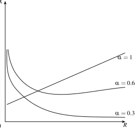
decreasing in the prize. To illustrate the effect of allowing for diminishing marginal returns in the prize sharezi, Figure 1 plots the players’ aggregate equilibrium effort against the size of the
prizeRfor different concavity parameters: we observe that the degree of concavity determines whether aggregate effort is monotonically increasing in the size of the prize, or not.
Using this example it is clear that if the structure of players’ preferences differ from the conventional structure, many of the main conclusions of contest theory may fail to hold. In this article we are interested in how contests are affected when players have alternative preference structures. As already mentioned, we show that the key to understanding contests with gen-eral preferences is the relationship between the rate of change of marginal rate of substitution between the prize share and effort.
2
Contests with general preferences
Consider a set of individual playersN={1, . . . ,n}that participate in a contest to obtain a rent, or prize, R. Their success in the contest is determined by their effort relative to the effort of other contestants and is given by the contest success function φ(xi,x−i), where xi denotes the
costly effort of playeri∈ Nandx−i denotes the vector of all other contestants’ effort levels. In this article we focus on contests in which the prize is perfectly divisible and is shared between contestants in accordance with the contest success function. Define zi as being contestant i’s allocation of the prize from the contest:
X
R
0
α=1
α =0.3
[image:5.595.166.434.62.323.2]α =0.6
Figure 1:Aggregate equilibrium effort in contests
We begin by studying a ‘simple’ Tullock contest for an exogenously-given prize of size R in which
φ(xi,x−i) =
(
xi
xi+X−i if X>0 or 1
n otherwise,
where X ≡ ∑j∈Nxj is the aggregate effort and X−i ≡ X−xi. Later in the article we consider
more general contest success functions, as well as situations in which the size of the prize is influenced by the effort of contestants, i.e., where the prize is endogenously determined by contestants’ efforts.
For each contestantiwe define a utility functionui(z,x)over their prize allocation from the contest, z, and their effort in contesting the prize, x. We denote MRSi(z,x) as contestant i’s
marginal rate of substitution betweenzandxsuch that:2
MRSi(z,x)≡ −u i x
ui z
.
Consider the(xi,zi)-space. Since utility is increasing inz but decreasing in effort, the indiffer-ence curves derived from the utility function defined above will have an upward slope (mea-sured by the marginal rate of substitution just defined) and utility is increasing in a north-west direction.
We focus on cases where (heterogenous) contestants’ utility is increasing in their allocation of the prize, at a decreasing rate; decreasing in effort, at an increasing rate; and if there are complementarities between the allocation of the prize from the contest and effort then these are sufficiently small.
Assumption 1. For each i∈ N, the utility function is differentiable as many times as required, uiz >0, ui
zz≤0, uix <0, uixx ≤0, and
uizx <min
MRSi u
i zz
,
1
MRSi
u
i xx
.
Concavity of the utility function is, of course, standard. The last condition in the assumption— which ensures complementarities betweenzandxare sufficiently small—implies that MRSzi >
0 andMRSi
x >0; to observe this note that
MRSiz =−u i
zuizx−uixuizz (ui
z)2
and MRSix =−u i
zuixx−uixuizx (ui
z)2
and therefore MRSiz > 0 ⇔ uizx < −MRSiuzzi and (noting thatuix < 0) MRSix > 0 ⇔ uizx < − 1
MRSiuixx.
Assumption 1 allows for a very broad class of preference structures. For instance, this framework nests the standard linear preference structure ui(z,x) = z−x, which is the dom-inant structure used within the contest literature. We can also capture convex costs of effort if we specified ui(z,x) = z−ci(x) with cix > 0,cixx > 0. The level of generality within our framework even allows for non-separable preferences betweenx andz allowing us to capture situations, where, for example, the marginal value of the prize is influenced by the effort exerted in contesting the prize. Thus by considering a general preference structure, our framework can not only provide an analysis that nests previous studies of share contests but also provides a tractable methodology by which to consider alternative and novel preference structures, which can be used to advance and expand the understanding and applicability of contests.
The dominant framework for exploring sharing contests in the literature has been to assume preferences are (quasi-)linear, with utility being linear in the share of the prize received. This means that existing studies have neglected to consider both diminishing marginal utility for contestants from their allocation of the prize, and complementarities between the effort in the contest and their enjoyment of the prize. To advance the analysis of contests toward a larger class of preference structures it is imperative to consider these issues.
3
Characterizing equilibria in Tullock contests with general
prefer-ences
We now turn to characterize equilibria in a simple Tullock contest over an exogenously-given perfectly divisible prize R. We seek a Nash equilibrium in the simultaneous-move game of complete information in which the player set is the contestants N= {1, . . . ,n}; their strategies are their choice of effort xi ∈ R+; and their payoffs are given by their utility of the contest outcomeui(z,x)wherex=xi andz= xi
xi+X−iR, which we assume satisfies Assumption 1. Note
that we allow all players to be heterogeneous, and we assumen≥2.
First, we note that at a Nash equilibrium of the contest each player may be seen as solving the problem
max
xi∈R+u
i
xi
xi+X−iR,x i
.
The necessary first-order condition forxito maximize utility givenX−i =∑j6=i∈Nxj, i.e. identify
a best response, is
X−i
(xi+X−i)2Ru
i
z+uix≤0, (2)
with equality ifxi >0.
Lemma 1. Suppose Assumption 1 is satisfied for a contestant, Then the first-order condition is both necessary and sufficient for identifying their best response.
Proof. The second-order sufficient condition is
uizx2 X−
i
(xi+X−i)2R+u
i zz
X−i (xi+X−i)2R
2
+uixx−uiz2 X−
i
For any xi > 0, the first-order condition implies (xi+XX−i−i)2R = −
ui x
ui
z = MRS
i. As such, the
second-order condition can be re-written
2MRSiuizx+MRSi
MRSiuizz+ 1
MRSiu i xx
− 2
xi+X−iMRS iui
z
<2MRSiuizx−MRSi
MRSi|uizz|+ 1
MRSi|u i xx|
<2MRSiuizx−2MRSimin
MRSi u i zz , 1 MRSi u i xx
=2MRSi
uizx−min
MRSi u i zz , 1 MRSi u i xx <0,
sinceuizx<minnMRSiuizz , 1
MRSi uixx
o
under Assumption 1.
Contestanti’s best response is thus given by bi(X−i;R) =max{0,xi}wherexi is the unique solution to
MRSi
xi
xi+X−iR,x i
= X− i
(xi+X−i)2R,
and we seek a Nash equilibrium in which players use mutually consistent best responses. Rather than working directly with best responses, we turn to analyze the contest using an extension of the ‘share function’ approach, as first developed by Cornes and Hartley (2005), to allow for general preferences. For each contestant we define a share function that gives their share of the prize that is consistent with a Nash equilibrium in which the aggregate effort of all contestants is X > 0. By replacing X−i with X−xi in the first-order condition (2) and letting
σi ≡xi/Xwe deduce that contestanti’s share function is given bysi(X;R) =max{0,σi}where σi is the solution to
li(σi,X;R)≡ MRSi(σiR,σiX)−(1−σi)R
X =0. (3)
Share functions shed light on individual behavior consistent with a Nash equilibrium: Xsi(X;R)
is the effort of contestanticonsistent with a Nash equilibrium in which the aggregate effort of all contestants is X > 0. To identify a Nash equilibrium, we require consistency at the aggre-gate level; that is, the sum of individual efforts being equal to the aggreaggre-gate effort, or for the sum of individual share functions to be equal to unity. Letting
S(X;R)≡
∑
j∈Nsj(X;R),
we have the following equivalence statement.
Lemma 2. In a contest with prize R, there is a Nash equilibrium with aggregate effort X∗ > 0if and only if
S(X∗;R) =1.
Proof. We seek to show that X∗ is a Nash equilibrium if and only if S(X∗;R) = 1. First, the “if” part. If X∗ is a Nash equilibrium then xi∗ = bi(X−i∗;R) for all i ∈ N. This implies
xi∗ = bi(X∗−xi∗;R) which in turn implies xi∗ = X∗si(X∗;R)for all i∈ N, and therefore that
X∗ = X∗∑j∈Nsj(X∗;R), and consequently S(X∗;R) = 1. For the “only if” part, note that for
eachi∈ N,X∗si(X∗;R) = bi(X∗−X∗si(X∗;R)). IfS(X∗;R) = 1 then X∗ =X∗S(X∗;R)and so
Questions of the existence and uniqueness of Nash equilibrium now rest on consideration of the behavior of the aggregate share function S(X;R), whose properties are derived from individual share functions, and its intersection with the unit line. The following proposition sets out the properties of individual share functions.
Proposition 1. For each i∈ N,
1. si(X;R)is a continuous function defined for all X >0and R.
2. si(X;R) → 1 as X → 0 and either si(X;R) = 0 for all X ≥ X¯i(R) ≡ R/MRSi(0, 0) if
MRSi(0, 0)>0or, if MRSi(0, 0) =0, si(X;R)→0as X →∞.
3. si(X,R)is strictly decreasing in X for0< X<X¯i(R).
Proof. 1. Recall from (3) that a contestant’s share function is implicitly defined as the value of
σi where
li(σi,X;R)≡ MRSi(σiR,σiX)−(1−σi)R
X =0,
ifσi is positive, otherwise the share function takes the value zero. Continuity of the share
func-tion is established by the assumed smooth nature of the funcfunc-tions in the first-order condifunc-tion. Next, note that
liσ=R MRSiz+X MRSix+ R
X >0, (4)
allowing us to conclude that there is at most one value of σi > 0 where li(σi,X;R) = 0, so
si(X;R)is a function.
2. When σi = 0, li(0,X;R) = MRSi(0, 0)−R/X. The fact just deduced thatlσi > 0 implies
that if li(0,X;R) ≥ 0 then li(σi,X;R) > 0 for all σi > 0, and therefore si(X;R) = 0. If
MRSi(0, 0)>0, ¯Xi(R)≡ R/MRSi(0, 0)is well-defined and we can conclude thatsi(X,R) = 0 for allX ≥ X¯i(R). If MRSi(0, 0) =0 then li(0,X;R) = −R/X. AsX→ ∞, li(0,X;R)→0 and
then the fact thatliσ>0 impliessi(X;R)→0.
As X → 0, Xli(σi,X;R) = XMRSi(σiR,σiX)−(1−σi)R → −(1−σi)R, so σi = 1 is the
only possibility to achieveli(σi,X;R) =0, implying si(X;R)→1.
3. Finally, to understand how share functions vary withXwe apply implicit differentiation to (3) to deduce that
siX =−lXi
li
σ
=− σ iMRSi
x+ (1−σi)XR2
R MRSi
z+X MRSix+ XR
<0, (5)
confirming the strict monotonicity.
The properties of individual share functions imply that in a contest with prize R the ag-gregate share functionS(X;R), being constructed from a sum of at least two individual share functions, exceeds 1 when X is small enough, is less than one when X is large enough, and is continuous and strictly decreasing in X implying there is exactly one value of X where
S(X;R) =1.
Proposition 2. In a contest with prize R there is a unique Nash equilibrium with aggregate effort X∗ such that
S(X∗;R) =1
in which the equilibrium effort of contestant i is xi =X∗si(X∗;R).
Proof. From Lemma 2 we know that Nash equilibria are identified by intersections of S(X;R)
with the unit line. From Proposition 1 we also know that individual share functions are single-valued, continuous and strictly decreasing in X > 0, and have the property si(X;R) → 1 as
Combined with the fact thatS(X;R)is continuous and strictly decreasing inX>0, this implies there is a single value of XwhereS(X;R) =1, and so the Nash equilibrium is unique.
As such, we confirm that in prize-sharing contests where players can have more general preferences over their allocation of the prize and the effort exerted in contesting the prize, the uniqueness of Nash equilibrium—as found in simple Tullock contests—is preserved under our stated assumptions.
4
The effect of the size of the contested prize
We now turn to investigate how contestants’ equilibrium behavior depends on the size of the prize they are contesting. We write X(R) for the equilibrium aggregate effort in a contest where the size of the prize isR, which is implicitly defined by
S(X(R);R) =1. (6)
To determine the sign of X0(R), we make use of expression (6) to deduce:3
X0(R) =−∑j∈Ns j R
∑j∈NsjX
(7)
Having already found that siX < 0 for all i ∈ N (Proposition 1), how equilibrium aggregate effort responds to a change in the size of the prize will rely on the features ofsjR, that we turn to investigate next.
Lemma 3.
siRR0⇔ziMRSiz−MRSiQ0.
Proof. Recall from (3) that a contestant’s share function is implicitly defined as the value of σi
where
li(σi,X;R)≡ MRSi(σiR,σiX)−(1−σi)R
X =0.
As such,
siR=−l i R
li
σ
=− σ iMRSi
z−(1−σi)X1
R MRSi
z+X MRSix+ RX
.
The denominator (as deduced in (4)) is positive. Noting that σiR = zi and that (1−σi)RX =
MRSi from the first-order condition, gives
siR =−wi(ziMRSiz−MRSi),
where wi = (R(R MRSi
z+X MRSix+ XR))−1 > 0, from whence the statement in the lemma
follows.
3Strictly speaking, we should not implicitly differentiate (6) since whilst it is continuous, where X = X¯i(R)
Putting the expression forX0(R)together with the expression forsi
R, it follows that
sgn{X0(R)}=−sgn{
∑
j∈N
wj(zjMRSzj −MRSj)}.
This allows us to draw the following conclusion regarding how the equilibrium aggregate effort in a contest changes with the size of the prize, which differs significantly from the standard conclusion for prize-sharing contests (that equilibrium aggregate effort always increases inR).
Proposition 3. Suppose the preferences of all contestants satisfy Assumption 1. If∑j∈Nwj(zjMRSzj−
MRSj) R 0 then X0(R) Q 0. A sufficient condition for this is for MRSi
zi to be increasing (constant,
decreasing) in zi for all contestants.
This proposition reveals that how aggregate effort changes with the size of the prize is crucially dependent on how the ratio MRSi/zi changes with the allocation of the prize (since the sign of the derivative of this object is equal to the sign of ziMRSi
z−MRSi). If MRSi/zi is
decreasing inzi for all contestants—as assumed in the contest literature so far as the marginal rate of substitution is constant inzi—then the equilibrium aggregate effort of contestants is al-ways increasing in the size of the contested prize. However, with our more general preferences
MRSi is increasing (weakly) inz, and if it increases sufficiently so that MRSi/zi also increases then aggregate effort may, in fact, decrease with a larger prize. This was the case in the moti-vating example at the start of the article and means that if we account for contestants having more general preferences in prize-sharing contests we must expel the conventional wisdom that larger prizes always command greater effort.
4.1 Interpreting the result
In a contest playerican be seen as solving the following constrained optimization problem:
max
xi∈R+u
i(zi,xi)s.t. zi = xi
∑j∈Nxj
R
Put differently, player imaximizes a utility function that is increasing in her share of the con-tested prize, zi, and decreasing in contest effort xi, subject to the constraint that implies her share of the contested prize is increasing in contest effort. This constraint can be interpreted as a budget constraint since it maps the combinations(zi,xi)that are achievable for a given R.
We have shown above that optimizing yields:
MRSi = X−x i
X2 R,
where the (positive) marginal rate of substitution equals the amount by which the budget constraint is being relaxed when contest effort increases. Bearing in mind that the marginal rate of substitution captures the relative increase of utility of marginally increasing the share of the contested prize enjoyed to marginally reducing the contest effort, we thus require that this relative increase in utility be equal to the relative relaxation of the budget constraint. This line of reasoning allows us to visualize the condition in (xi,zi)-space where we represent player
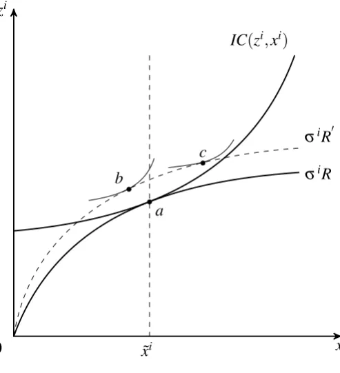
i’s (upward-sloping) indifference curves and budget constraint. Accordingly, at optimality, for playerito be attaining the highest indifference curve for a given budget constraint, the slopes of these two loci are equal, as illustrated in Figure 2, where pointa depicts the tangency between the budget constraint and an indifference curve.
Increasing the value of the prize (to R0) relaxes the budget constraint since it enables any player i to increasezi, while keeping xi constant. Since the slope of the BC equals XX−2xiR, an
zi
xi
0
σiR0
σiR
IC(zi,xi)
˜
xi
a b
[image:11.595.171.418.60.331.2]c
Figure 2:Equilibrium effort
the BC. To determine whether playeri’s effort will increase or decrease with a change in R, it is thus sufficient to look at the change of the slope of the indifference curve, when increasing
Rwhile maintainingxi constant. Should this slope increase by more than the slope of budget constraint, this will imply that with a higher value of the prize R, player i will be able to increase his consumption ofzi while expendinglesscontest effort. Should the opposite hold, at the new equilibrium more contest effort will be exerted by playeri. Mathematically, the relative change in slopes is such that we witness a decrease of contest effort at equilibrium if:
∂MRSi(σiR,xi) ∂R >
∂X−x
i
X2 R
∂R ⇔σ
iMRSi z >
X−xi X2 .
Utilizing (2), we deduce that XX−2xi = MRSi/R and therefore we can re-write the above
expression (noting thatσiR=zi) as
MRSi−ziMRSiz <0, (8)
which is exactly the same condition driving the result of Proposition 3.
Referring back to Figure 2, if an increase in the value of the prize R is accompanied by inequality (8) being satisfied, this will lead to a reduction of individual contest effort as reflected by pointb. If on the other hand, the inequality is violated, then individual effort will increase, as reflected by pointc.
Thus, we find that an increase in the value of the prize in a Tullock share-contest with general preferences may result in increases or decreases of individual contestants’ efforts, de-pending on their preferences. To better understand why the literature unambiguously identifies a positive relationship, we further explore inequality (8) by computing the components of the object on the left:
MRSi−ziMRSiz = u i
xuiz−zi uixuizz−uizuizx
(ui z)
2 (9)
their share if the prize, while the cost of effort is assumed to be (weakly) convex: ui(z,x) =
z−ci(x). Imposing such assumptions implies that uizz = uizx = 0 anduixx ≤0, so that the sign of expression (9) is unambiguously positive. Accordingly this implies a positive relationship between the value of the prize and individual contest effort.
From Condition (9), we realize that additive separability (uizx = 0) is not the defining fac-tor behind the monotonic relationship between prize-value and contest effort found in the literature. Indeed, diminishing marginal returns inzi (uizz <0) proves sufficient to yield a non-standard relationship between the value of the prize and effort even with additively separable utility functions.
On the other hand, neither are diminishing marginal returns on zi a necessary condition for obtaining a non-monotonic relationship between prize-value and contest effort. Consider Condition (9) once more, and setui
zz=0. In the presence of sufficiently strong substitutability
betweenzi andxi, increases inRmay generate decreases in contest effort. Strong substitutabil-ity implies that higher contest effort strongly reduces the marginal utilsubstitutabil-ity of the prize-share.
5
The dissipation ratio
We now consider how the dissipation ratio alters under a Tullock contest with general prefer-ences. Recall that the share function satisfies the first-order condition
MRSi(σiR,σiX) = (1−σi)R
X,
and let D= X
R be the dissipation ratio. Noting thatX =D·R, we can write the share function
assi(DR,R)which will satisfy
li(σi,DR;R)≡ MRSi(σiR,σiDR)−(1−σi)1
D =0.
Then the equilibrium dissipation ratio, writtenD(R), must satisfy
∑
j∈N
sj(D(R)R,R) =1.
How the dissipation ratio changes in the size of the prize can be derived as follows:
D0(R) =−∑j∈N
dsi dR
∑j∈N ds
i dD
(notice that the change from partial derivatives as, in particular,Renters both arguments of the share function). Now,
dsi
dR =−
dli dR
li
σ
and ds
i
dD =−
dli dD
li
σ
.
We deduce that
liσ= 1
σi
ziMRSiz+xiMRSix+ σ i
D
,
dli
dD =σ
iR
·MRSix+1−σ i
D2 and
dli
dR =
1
R(z
iMRSi
z+xiMRSix).
Under Assumption 1, each of these expressions is non-negative, and therefore we deduce that
D0(R) ≤ 0, and is exactly zero only whenziMRSi
z+xiMRSix = 0 for all contestants, as in the
size of the prize in our general case, it does not increase at a rate such thatD(R) = X(R)/R
also increases. In Tullock contests with linear preferences the dissipation ratio is constant; our result confirms that under more general preferences the same result as in contests with convex costs—that the dissipation ratio decreases in the size of the prize—also holds. Our findings thus complement the literature that attempts to explain the existence of under dissipation, such as justified by loss aversion (Cornes and Hartley, 2003) and behavioral considerations (Baharad and Nitzan, 2008).
6
Extensions
In this section we pursue two generalizations of our model of contests with general preferences: the first allows for a more general contest success function; and the second allows for the prize to be endogenously determined by contestants’ efforts.
6.1 General contest success function
So far, we have considered a simple Tullock contest in which the contest success function has taken the form φ(xi,x−i) = xi+xXi −i. Of course, Tullock contests can be more general than this,
typically considering an additional parameterr, and specifying φ(xi,x−i) = (x
i)r
(xi)r+∑
j6=i∈N(xj)r. To
capture this, we will follow Cornes and Hartley (2005) and specify that
φ(xi,x−i) = P
i(xi)
∑i∈NPi(xi)
, (10)
where we need to assume thatPi0 >0 andPi00 ≤0.4
We now need to re-consider our analysis with this more general contest success function. According to (1), zi = Pi(xi)
∑iPi(xi)R. So that the share function approach can be utilized, let us
change the variable of consideration and rather than focus on effort, xi, let us think of contes-tants choosing what Cornes and Hartley (2005) call the contestant’s “input” yi = Pi(xi), from
which effort can be derived since xi = Pi−1(yi) and the contest ‘technology’ is assumed to be monotonic so the inverse of Pi(·)is a singleton. With this change of variables, contestants can be seen as choosing their input to maximize their payoff ui(zi,Pi−1(yi)), where their share of
the prize iszi = yYiR(Ybeing the aggregate input∑j∈Nyj).
The first-order condition of this optimization problem that characterizes a contestant’s input best response is
Y−i
(yi+Y−i)2Ru
i
z+Pi−1uix ≤0
with equality if yi > 0. Replacing Y−i with Y−yi and letting ˆσi = yi/Y, this can be used to
define the contestant’s share function as ˆsi(Y;R) = max{0, ˆσi} where, making the arguments
of functions explicit, ˆσi is the solution to
ˆ
li(σˆi,Y;R)≡ MRSi(σˆiR,Pi−1(σˆiY))Pi−1(σˆiY)−(1−σˆi)R
Y =0. (11)
As with our previous analysis, we can use share functions to shed light on the properties of Nash equilibrium in the contest, since there is a Nash equilibrium with aggregate inputY∗ if and only if∑j∈Nsˆj(Y∗;R) = 1, in which contestanti’s input isyi∗ =Y∗sˆi(Y∗;R)and therefore their contest effort is xi∗ =Pi−1(Y∗sˆi(Y∗;R)).
4This implies that our CSF tracks the general function axiomatized by Skaperdas (1996) up to the difference that
As with our simple contest, we can deduce that individual share functions ˆsi(Y;R) are indeed functions that are continuous and strictly decreasing on Y > 0. To deduce this, note that
ˆ
lσˆi = (R·MRSzi +YPi−10MRSix)Pi−1+MRSiYPi−10+ R
Y >0
and
ˆ
liY =Pi−1σˆiPi−10MRSix+MRSiσˆiPi−10+ (1−σˆi)R
Y2 >0,
so the analog of Proposition 1 follows for this case.
Then let us define the aggregate equilibrium input as a function of the contested prize as
Y(R)which will satisfy
∑
j∈N
ˆ
sj(Y(R);R) =1.
Then we turn to consider how the aggregate input varies with the size of the contested prize, noting (with our usual apology for using implicit differentiation at parts of the domain where we should not) that
Y0(R) =−∑j∈Nsˆ j R
∑j∈Ns j Y
,
and therefore
sgn{Y0(R)}=sgn
(
∑
j∈N
ˆ
sjR
)
.
For each contestanti, ˆsi
R= −lˆRi/ˆliσˆ and therefore sgn{sˆ
i
R}=−sgn{lˆiR}. Now,
ˆ
liR =σˆiMRSizPi−1−(1−σˆi)1
Y
= 1
R
ˆ
σiR·MRSizPi−1−(1−σˆi)R
Y
= P i−1
R (z
iMRSi
z−MRSi),
where the last line exploits the first-order condition. As such,
sgn{sˆiR}=sgn{MRSi−ziMRSiz},
and therefore we can conclude that
Y0(R)Q0⇐ MRSi−ziMRSiz Q0 ,∀i∈ N
which is implied by the ratioMRSi/zi being increasing (constant, decreasing) inzi.
As such, we conclude that the aggregateinputinto the contest can vary with the size of the prize in much the same way as the aggregate effort in a simple Tullock contest. However, we wish to make conclusions about the aggregate effort in this more general case, which cannot be directly deduced from the aggregate input. Since X = ∑j∈Nxj where xi = Pi−1(yi), to be
sure of the change in aggregate effort, we need to make sure each individual contestant’s effort changes in the same direction, which requires each contestant’s input to change in the same direction. Of course, if we assume homogeneous contestants this is obvious, but we do not do so.
Now consider how individual inputs change. Writing ˆyi(Y(R);R) = Y(R)sˆi(Y(R);R), we find that
d ˆyi(Y(R);R)
dR =sˆ
iY0+Y(sˆi
YY0+sˆiR) =Y0(sˆi+YsˆiY) +YsˆiR.
SinceMRSi−ziMRSi
z <0 andY0 <0, we will have
d ˆyi(Y(R);R)
dR Q0 if ˆsi+YsˆiY >0. Since ˆsiY <0
this is not obvious, but if we decompose this expression, we can indeed conclude that it is true. For,
ˆ
σi+YsˆiY =σˆi−
YσˆiPi−10(pi−1MRSix+MRSi)(1−σˆi)RY
Pi−1(R·MRSi
z+YPi−10MRSix) +MRSiYPi−10+ RY
= σˆ
iRMRSi
zPi−1+σˆi RY −(1−σˆi)RY
Pi−1(R·MRSi
z+YPi−10MRSix) +MRSiYPi−10+ RY
by putting terms over a common denominator and cancelling. Now, the first-order condition can be exploited to reduce the numerator of this expression to
Pi−10(ziMRSiz−MRSi) +σˆiR
Y
which is positive when MRSi−ziMRSiz < 0. Combined with a positive denominator, this allows us to conclude that when MRSi−ziMRSiz < 0 for alli∈ N, not only isY0(R)< 0 but
d ˆyi(Y(R);R)
dR <0 for alli∈ Nwhich implies that each individual contestant’s effort will be lower,
and therefore aggregate effort will reduce.
6.2 Endogenous rent
We now turn to consider the case where the contested rent is not fixed, but is influenced by the effort of contestants. So that we can consider different rent-generating technologies and understand the effect on equilibrium effort from contestants, we define the rent asR= f(X,α)
where α is interpreted as a productivity parameter and is such that fα > 0. Whilst we allow
for the rent to be increasing or decreasing in aggregate effort5, we do impose the following assumption.
Assumption 2. f(X,α)is a continuous function that is differentiable as many times as required and
fXX ≤0. We also impose the technical assumptionslimX→∞ fX≯0;|fXX|is finite∀X; and, if fX <0
then for each contestant for whom MRSiz> 0, fX > fXX−MRS
i x
MRSi z .
According to (1),zi = xi
xi+X−i f(xi+X−i;α)and the first-order condition that will be used to
identify a contestant’s best response is:
uiz
x−i
(xi+X−i)2f(x
i+X−i;
α) + x
i
xi+X−i fX(x
i+X−i;
α)
+uix ≤0 (12)
with equality ifxi >0.
In the next lemma we demonstrate the concavity of the optimization problem contestants may be seen as facing.
Lemma 4. Suppose Assumptions 1 and 2 are satisfied. Then the first-order condition is both necessary and sufficient for identifying a contestant’s best response.
5Not restricting f
Xto be positive enables us to capture with our model the case of Cournot competition where
Proof. Omitting the arguments of functions and using the simplifying notation X = X−i+xi
andσi = xi/X, the second derivative of the objective function is
uizz
(1−σi)f
X +σ
if X
2
+uixx+2uizx
(1−σi) f
X +σ
if X
+uiz
−2(1−σi)
X
f X − fX
+σifXX
Since function f(X;α)is concave, f/X > fX, ∀X >0, thus implying that the forth term of the
above expression is necessarily negative. It is thus sufficient to show that:
uizz
(1−σi) f
X +σ
if X
2
+uixx+2uizx
(1−σi) f
X +σ
if X
<0
Since the first-order condition implies MRSi = (1−σi)f
X +σifX, the above expression can be
written as:
uizzhMRSii2+uxxi +2uizxMRSi <0
Following the steps of the proof of Lemma 1, we deduce that this inequality is satisfied given Assumption 1.
Adopting the same approach as in the rest of the paper, contestanti’s share function in this contest, that we write ˜si(X;α), is given by ˜si(X;α) =max{0,σi}, whereσi is the solution to:
˜
li(σi,X;α)≡ MRSi(σif(X;α),σiX)−(1−σi)f(X;α)
X −σ
if
X(X;α) =0. (13)
We seek a Nash equilibrium of the contest that we identify by the aggregate effortX∗such that ∑j∈Ns˜j(X∗;α) =1.
Following the reasoning of our previous analysis, we can establish the analog of Proposition 1 that elucidated the properties of share functions for the standard case.
Proposition 4. Suppose Assumptions 1 and 2 are satisfied. Then for each contestant i∈ N,
1. s˜i(X;α)is a function defined for all X >0andα;
2. s˜i(X;α) → 1 as X → 0, and either s˜i(X;α) = 0 for all X ≥ X¯i(α)where X¯i(α) is such that
MRSi(0, 0) = f(X¯i(α);α)/ ¯Xi(α)if MRSi(0, 0) > 0, or if MRSi(0, 0) = 0, s˜i(X;α) → 0as
X →∞.
3. s˜i(X;α)is strictly decreasing in X for0<X< X¯i(α).
Proof. 1. Note that:
˜
lσi = f(X;α)MRSzi +XMRSix+ f(X;α)
X − fX(X;α)>0
where the sign follows from the concavity of f(X;α) which implies f(X;α)/X > fX(X;α).
This in turn implies that there is at most one value ofσi where ˜li(σi,X;α) =0, so ˜si(X;α)is a
function.
2. When σi =0, ˜li = MRSi(0, 0)− f(XX;α). Since ˜lσi > 0, if ˜li(0,X;α)≥ 0, then ˜li(σi,X;α)> 0
for all σi > 0, and therefore ˜si(X;α) = 0. As such, if MRSi(0, 0) > 0, defining ¯Xi(α) as in
the proposition allows us to define ˜si(X;α) = 0 for all X ≥ X¯i(α). If MRS(0, 0) = 0, then
˜
li(0,X;α) = −f(XX;α). As X → ∞, and since limX→∞ fX ≯ 0, f(x;α)/X → 0 and the fact that
˜
lσi >0 implies ˜si(X;α)→0.
AsX→0, we show that Xl˜i(σi,X;α)→0 when σi =1. Consider the following expression:
Xl˜i(σi,X;α) =X
MRSi(σif(X;α),σiX)−σif(X;α)
X
+X
f(X;α)
X −σ
if
X(X;α)
This is composed of two terms. Focusing on the first term, as X → 0, since f(X;α) → 0,
the entire term tends to zero. Looking next at the second term. One candidate for satisfying
Xl˜i(σi,X;α) = 0 is that lim
X→0{f/X−σifX}= 0. Showing this is equivalent to showing the
following:
lim
X→0
f(X;α)
X
σifX
= lim
X→0
f(X;α) σiX fX
=1 (14)
Since the limit of this expression is indeterminate, we apply l’Hospital’s rule to obtain:
lim
X→0
f(X;α) σiX fX
= lim
X→0
fX
σi[fX+X fXX]
Since fXX ≤0 and is finite, we conclude that:
lim
X→0
f(X;α) σiX fX
= 1
σi
Thus implying that for equation (14) to be satisfied we requireσ =1. Since ˜lσi >0, there exists
at most one value ofσi satisfying the equality, thus implying that ˜si →1.
3. Applying implicit differentiation to (13) we deduce that:
˜
six =−l˜ix
˜
li
σ
=−σ if
XMRSiz+σMRSix−(1−σi)
X f X−f
X2
−σfXX
f MRSi
z+XMRSix+ Xf − fX
(15)
Since the denominator is positive, to establish the sign of (15) we thus need to determine the sign of the numerator, showing it is positive. Note first that−(1−σi)
X fX−f
X2
= 1−σi
X
f X− fX
>
0 by concavity of f. Now, since fX is allowed to take negative values, for (15) to be positive it
is sufficient to establish the numerator is positive for the case whereσi =1, i.e. the case where
the highest weight is being allocated to fX. We thus need to ensure that:
fXMRSiz+MRSix− fXX >0⇒ fX>
fXX−MRSix
MRSi z
,
which is assumed of the rent-generation technology.
We now explore the effect of productivity on individual and aggregate contest effort. In a contest with endogenous prize determination, the aggregate effort consistent with a Nash equilibrium is given by ˜X(α)which is defined such that
∑
j∈N
˜
sj(X;α) =1.
Applying implicit differentiation (again with apology) we deduce that the effect of a change in the way rent is generated on equilibrium aggregate effort is given by
˜
X0(α) =−∑j∈N
˜
sjα
∑j∈Ns˜ j X
.
Having already shown that the denominator is negative in the previous proposition, we deduce that the sign of this expression is equal to the sign of the numerator. The next lemma establishes the condition determining how individual shares vary with the productivity pa-rameter:
Lemma 5. Suppose Assumptions 1 and 2 are satisfied. Then
˜
siα R0⇔ 1
f
fα(ziMRSiz−MRSi) +σi(fαfX− f fXα)
Proof. Applying implicit differentiation to (13), we obtain:
˜
siα =−l˜ i
α
˜
li
σ
Having already established that ˜lσi <0, sgn{s˜αi}=sgn{l˜iα}. Now,
˜
lαi = σifαMRS
i
z−(1−σi)
fα
X −σifXα
= z if
αMRSiz
f −
h
(1−σi)Xf +σifX
i
fα
f +σ
i fXfα
f −σi fXαf
f
= 1
f
fα(ziMRSiz−MRSi) +σi(fαfX− f fXα)
.
This condition is slightly more elaborate than the one identified in the previous settings, and given that we allow for fX < 0, we obtain that for individual contest effort to decrease
with productivity it is not anymore sufficient forziMRSzi > MRSi.
Interestingly, for an entire category of production functions, we obtain that a necessary and sufficient condition for determining how individual effort varies with productivity is the same as in our benchmark model. More specifically, for any function admitting an effort-augmenting productivity such that f(X;α) =αg(X), withg0(X)R0 andg00(X)<0, we obtain
fαfX− f fXα =αgg0−αgg0 =0.
More generally, how effort varies with the productivity parameter requires conditions that combine properties of the rent generation function with conditions on preferences, where our condition on the direction of change of the ratio of the marginal rate of substitution to the prize share is of fundamental importance.
7
Conclusions
The purpose of this article is to investigate contests allowing for contestants to have more gen-eral preferences than have been assumed in existing treatments. We focus on heterogeneous players competing in share contests and prove the existence and uniqueness of a Nash equi-librium. Our main aim is to discover the links between the features of contestants’ preferences and the features of the contest equilibrium.
In the conventional literature—where players have (quasi-)linear preferences—aggregate contest efforts are increasing in the prize. We find that when preferences are allowed to be more general than this, and in particular when contestants have diminishing marginal utility over their prize share, this familiar result may no longer hold. We show a key determinant within the contest equilibrium is the rate of change of the marginal rate of substitution between players’ share of the prize and their sunk effort. We not only investigate this relationship in a simple Tullock contest, but also in the case of more general contest success functions, and where the prize is endogenously determined.
This encompassing framework now allows the study of contests with much more general preferences and thus increases the applicability of the contest model.
References
Congleton, R., Hillman, A., and Konrad, K. (2008) 40 Years of Rent-Seeking Research: Springer Verlag.
Cornes, R. and Hartley, R. (2003)Loss aversion and the Tullock paradox: Department of Economics, University of Nottingham.
Cornes, R. and Hartley, R. (2005) “Asymmetric contests with general technologies,” Economic Theory,26, pp. 923–946.
Cornes, R. and Hartley, R. (2012) “Risk aversion in symmetric and asymmetric contests,” Eco-nomic Theory,51, pp. 247–275.
Hillman, A. L. and Katz, E. (1984) “Risk-averse rent seekers and the social cost of monopoly power,”The Economic Journal,94, pp. 104–110.
Hillman, A. L. and Samet, D. (1987) “Dissipation of contestable rents by small numbers of contenders,”Public Choice,54, pp. 63–82.
Konrad, K. A. (2009)Strategy and dynamic in contests, Oxford: Oxford University Press.
Konrad, K. and Schlesinger, H. (1997) “Risk aversion in rent-seeking and rent-augmenting games,”The Economic Journal,107, pp. 1671–1683.
Long, N. V. and Vousden, N. (1987) “Risk-averse rent seeking with shared rents,”The Economic Journal,97, pp. 971–985.
Skaperdas, S. (1996) “Contest success functions,”Economic Theory,7, pp. 283–290.
Skaperdas, S. and Gan, L. (1995) “Risk aversion in contests,” The Economic Journal, 105, pp. 951–962.