City, University of London Institutional Repository
Citation
:
Haslip, G. G. & Kaishev, V. K. (2014). Lookback option pricing using the Fourier transform B-spline method. Quantitative Finance, 14(5), pp. 789-803. doi:10.1080/14697688.2014.882010
This is the accepted version of the paper.
This version of the publication may differ from the final published
version.
Permanent repository link:
http://openaccess.city.ac.uk/11975/Link to published version
:
http://dx.doi.org/10.1080/14697688.2014.882010Copyright and reuse:
City Research Online aims to make research
outputs of City, University of London available to a wider audience.
Copyright and Moral Rights remain with the author(s) and/or copyright
holders. URLs from City Research Online may be freely distributed and
linked to.
City Research Online: http://openaccess.city.ac.uk/ [email protected]
Lookback Option Pricing Using the Fourier
Transform B-spline Method
GARETH G. HASLIP
∗†
& VLADIMIR K. KAISHEV
∗∗†
†
Faculty of Actuarial Science and Insurance, Cass Business School, City
University London, 106 Bunhill Road, London EC1Y 8TZ, United Kingdom
(11 November 2013)
We derive a new, efficient closed-form formula approximating the price of discrete lookback options, whose underlying asset price is driven by an exponential semimartingale process in-cluding (jump) diffusions, L´evy models, affine processes and other models. The derivation of our pricing formula is based on inverting the Fourier transform using B-spline approximation theory. We give an error bound for our formula and establish its fast rate of convergence to the true price. Our method provides lookback option prices across the quantum of strike prices with greater efficiency than for a single strike price under existing methods.
We provide an alternative proof to the Spitzer formula for the characteristic function of the maximum of a discretely observed stochastic process, which yields a numerically efficient algorithm based on convolutions. This is an important result which could have a wide range of applications where the Spitzer formula is utilized.
We illustrate the numerical efficiency of our algorithm by applying it in pricing fixed and floating discrete lookback options under Brownian motion, jump diffusion models, and the variance gamma process.
Keywords:Lookback option pricing, Fourier transform, B-spline interpolation, Spitzer formula, jump diffusion, variance gamma
1. Introduction
Lookback options are among the most popular path dependent exotic options traded over-the-counter or embedded in structured notes or insurance contracts. The lookback option provides a payoff at expiry that depends on the continuously or discretely monitored extremum of the underlying asset over the lifetime of the contract. Discrete lookback options commonly arise in life insurance applications, since they feature in variable annuity and equity indexed annuity contracts, which are popular in North America. Lin and Tan (2003) note that these protection features appeal to investors of savings products, but also are a source of significant volatility for
∗Corresponding author. Email: [email protected]
∗∗Corresponding author. Email: [email protected]
Quantitative Finance
ISSN 1469-7688 print/ISSN 1469-7696 online c⃝200x Taylor & Francis http://www.tandf.co.uk/journals
insurance companies that underwrite the product. Wong and Lam (2009) consider the valuation of dynamic fund protection in the context of equity indexed annuities. In particular, the valuation of the embedded options have not always been carried out using market consistent principles.
The theory for pricing continuously monitored lookback options is well developed, and a variety of methods exist under popular continuous-time asset price models. For example, Goldmanet al.
(1979b), Goldman et al. (1979a), and Conze and Viswanathan (1991) obtain closed-form prices under the Black-Scholes model assumptions. More recently, Boyle and Tian (1999) and Linetsky (2004) consider pricing continuous lookback options under the Constant Elasticity of Variance model of Beckers (1980). Kou and Wang (2004) and Cai and Kou (2011) consider pricing options under the Laplace transform (LT), where asset prices follow the double exponential jump diffusion model of Kou and Wang (2004) and the mixed exponential jump diffusion model. The latter was first considered by Lipton (2002a), and more recently by Cai and Kou (2011).
In contrast to the continuous case, the development of the theory of pricing discrete lookback options has been slower and relies largely on numerical methods. Heynen and Kat (1995) demon-strate that approximating discrete lookback options in terms of their continuous counterparts can lead to significant pricing errors, and Broadie et al. (1999) provide a detailed comparison of pricing continuous and discrete lookback options. Pricing of discrete lookback options has devel-oped in several stages. Initially, pricing methods were based around (i) binomial methods, see, for example, Babbs (1992) and Hull and White (1993), (ii) partial differential equations (PDE), as shown by Wilmott et al. (1993) and Forsyth et al. (1999), and (iii) numerical integration in AitSahlia and Lai (1997) and Tse et al. (2001). Further extensions to the lattice based methods are proposed by Broadieet al.(1999) and Foufas and Larson (2004) that suggest a finite element based PDE methodology. However, with the exception of Tse et al. (2001), these methods focus on the Brownian motion model and are not easily extended to other models of asset return.
The next major breakthrough in the pricing of discrete lookback options was made by ¨Ohgren (2001), who used the Spitzer identity to derive a recurrence formula for the evaluation of the characteristic function of the discretely monitored maximum asset price. The latter recurrence was used by ¨Ohgren (2001) to price discrete lookback options at inception or at a monitoring point. This is an important result that Petrella and Kou (2004) and Borovkov and Novikov (2002) extend to a range of stochastic models, including the Black and Scholes (1973) model, and jump diffusion models, such as Merton (1976) and Kou (2002). Furthermore, Petrella and Kou (2004) extend the pricing method to value discrete lookback options at any point in time, not just at inception or at a monitoring point. It should be noted that related fluctuation identities were considered by Lipton (2002a) in the context of pricing path-dependent options. More recently, Broadie and Yamamoto (2005) propose a new pricing framework that utilizes the Fast Gauss Transform and demonstrate its use for pricing under the Merton (1976) jump diffusion model. Yamamoto (2005) applies this framework to pricing under the double exponential jump diffusion model of Kou and Wang (2004). Finally, two new pricing frameworks have been developed more recently. First, Atkinson and Fusai (2007) develop a method based on solving a Wiener-Hopf integral equation and show how this is closely related to the Spitzer formula. They provide a semi-closed-form solution for the option price under the Black-Scholes setting, and Green et al.
(2010) propose that this methodology can be applied to other L´evy models. Second, Feng and Linetsky (2009) propose an approach based on the Hilbert transform and demonstrate that it provides efficient and accurate prices for a range of L´evy models, including the double exponential jump diffusion process.
(see also Lewis (2000)), who applies the inverse Fourier transform to provide an option valuation formula as a contour integral in the complex plane. It should be noted that a similar approach to Lewis (2001) is described by Lipton (2002b) in the context of FX option pricing (see also Lipton (2001)). The Lewis-Lipton approach generalizes the method of Carr and Madan (1999) since their dampening factor corresponds to the path of the contour integral in the Fourier transform. Generalizations of the Lewis-Lipton framework have recently been considered by Dufresneet al.
(2009) and by Eberleinet al.(2010). The latter authors have shown that the Lewis-Lipton option pricing framework is valid for the more general class of exponential semimartingale models of the underlying asset price dynamics. This class is rich and encompasses the majority of models utilized in finance for pricing derivatives. Examples include (i) the general families of (jump) diffusion processes such as the Black and Scholes (1973) model, the Merton (1976) model and the mixed exponential model of Lipton (2002a), and (ii) pure jump L´evy processes such as the CGMY processes of Carr et al. (2002), the generalized hyperbolic models (see Eberlein (2001)), and the general class of linear combinations of gamma (LG) processes, recently introduced by Kaishev (2013), which includes as special cases, the variance gamma (VG) process introduced by Madanet al. (1998), and the bilateral gamma process considered by K¨uchler and Tappe (2008). For properties of some of the particular examples of semimartingale models see Eberlein et al.
(2008).
The FTBS method uses B-spline approximation theory to provide an accurate closed-form approximation to a Fourier transform representation of the discrete lookback option price. In common with Petrella and Kou (2004) and Borovkov and Novikov (2002), our method is based on the idea of applying the Spitzer formula to obtain the characteristic function of the discretely observed maximum asset price. A key advantage of the FTBS method is that it enables the valuation of discrete lookback options across a large number of strike prices in a single procedure with greater efficiency than for a single strike price under the methods of either Petrella and Kou (2004) or Borovkov and Novikov (2002). The FTBS method for pricing lookback options is an extension of the framework described in Haslip and Kaishev (2013) for pricing European options. Several key innovations are introduced in this paper. First, we apply the Fourier transform of Lewis (2001) and Lipton (2002b) as extended by Eberleinet al. (2010) to obtain a semi-closed-form pricing semi-closed-formula for discrete lookback options in terms of the characteristic function of the maximum of the underlying log-return process (see Proposition 2), Second, we propose a new con-volution algorithm (see Algorithm 1) for computing the characteristic function of the maximum, which is based on the Spitzer-recurrence expansion formula (see Theorem 4.1). The latter first appears in Wendel (1958) (see equation (1a) therein), but has since then remained unknown in the quantitative finance literature. In Theorem 4.1, we provide a new, simple proof of this formula (see Appendix B.1), and show that it gives rise to a new efficient, convolution based algorithm (see Algorithm 1) for the computation of the characteristic function of the maximum. We then apply it to evaluate the characteristic function of the maximum of the underlying log-return process over a large number of monitoring points. This provides a significant efficiency improvement over the Spitzer recurrence formula of ¨Ohgren (2001). Third, we use B-spline interpolation theory to develop a strike-separable pricing formula that enables valuation of lookback options across a large number of strike prices in a single procedure with greater efficiency than for a single strike price under the methods of either Petrella and Kou (2004) or Borovkov and Novikov (2002). Finally, using residue calculus, we apply the FTBS method for efficient pricing of discrete lookback options under the VG process.
Lev-endorski˘ı and Xie (2012), the Cosine method of Fang and Oosterlee (2008), and the Convolution method of Lordet al.(2008).
The paper is structured as follows. In Section 2, we first introduce the discrete lookback option, and then the Lewis-Lipton Fourier transform framework as extended by Eberlein et al. (2010), and use it to derive a discrete lookback option pricing formula (see Proposition 2.3). In Section 3 we develop our FTBS method for pricing discrete lookback options. In Section 3.2, we introduce a B-spline interpolation method by means of which we obtain our main result, the closed-form, Fourier transform B-spline discrete lookback option pricing formula given in Theorem 3.3. The latter theorem involves the characteristic function of the discretely observed asset price maximum. In order to efficiently evaluate this characteristic function, in Theorem 4.1 of Section 4.1, we derive an explicit expansion representation for it, based on the Spitzer recurrence formula (23), given by
¨
Ohgren (2001). We use the result of Theorem 4.1 which first appears in Wendel (1958) to develop an efficient convolution based algorithm (see Algorithm 1) for the evaluation of the characteristic function of the underlying log-return process. In Section 4.2, we provide a Fourier transform representation of the coefficients in the Spitzer-recurrence expansion representation formula given by Theorem 4.1. In Section 5 we illustrate how the FTBS method is applied to several popular models for the underlying asset price movement. Section 6 summarizes the numerical results and Section 7 provides conclusions and discussion. Proofs and auxiliary materials are given in Appendices A-B.
2. Discrete Lookback Options
In this section, we describe our proposed framework for pricing discrete lookback options. The risk-neutral dynamics of the asset price are modeled using an exponential semimartingale process given byS(t) =S(0)eLt, whereS(t) is the asset price at timet≥0, and L
t is a semimartingale process describing the log-return under probability measureQ. We refer the reader to, for example, Jacod and Shiryaev (2003), for a primer on semimartingale processes. For brevity, we refer to discretely monitored lookback options simply as lookback options throughout this paper.
2.1. Notation and Background
Let T denote the expiry time of the lookback option and [T0, T] be the lookback period over which the asset price is observed at q+ 1 evenly spaced monitoring times, tj =T0+ T−qT0j, for j = 0, . . . , q. The asset price at time tj is denoted Sj = S(tj) = S(0)eLtj. Let j∗ be such that tj∗ ≤t < tj∗+1, where t is the current time (T0 ≤t≤T). We denote the maximum value of the asset price realized fromT0 to tover the discrete monitoring times,tj, j = 0, . . . , j∗, by
M = max
j= 0, . . . , j∗
S(tj). (1)
We denote by Xk = maxj=1,...,kLj∗+j the observed future maximum log-return process over the monitoring timestj∗+1, . . . , tj∗+k for k= 1, . . . , q−j∗. To simplify the notation, denote bym the number of future monitoring time points, i.e.m=q−j∗. Several different types of lookback options exist, and without loss of generality in this paper we consider (i) the fixed-strike lookback call option, and (ii) the floating lookback put option. The pricing theory for the fixed-strike lookback put option and the floating lookback call option are similar and require only minor modification of the results presented in this paper.
call with strike price K and floating put lookback options are (i) (maxi=0,...,qSi−K)+, and (ii) maxi=0,...,qSi−ST, respectively. However, as highlighted by Petrella and Kou (2004), it is also important to be able to price a lookback contract at some current timet, after the time of inception, T0, i.e., when T0 < t < T. In this case, the payoff will be dependent on the observed maximum, M since inception. The following proposition explains how to price lookback options at any point in time by conditioning on the observed discrete extremum until the last monitoring point.
Proposition 2.1 Valuation of Lookback Options: The price at the current time t(T0 ≤t≤T)
of a fixed lookback call option, F C(t, T), and floating lookback put option, LP(t, T), that expires at future timeT >0and were incepted at time T0 in the past are given by
F C(t, T) =
S0e−r(T−t)EQ
[(
eXm− K
S0
)+]
, ifM < K
S0e−r(T−t)EQ
[(
eXm− M
S0
)+]
+ (M−K)e−r(T−t), ifM ≥K
(2)
LP(t, T) =
S0e−r(T−t))EQ
[
eXm]−S
0, ifM ≤S0
S0e−r(T−t)
{
EQ
[
eXm]+E
Q
[(
M S0 −e
Xm
)+]}
−S0, ifM > S0,
(3)
respectively, whereM = max j=0, ... ,j∗
S(tj) and r is the risk-free rate of interest.
Proof: The valuation formula forF C(t, T) andLP(t, T) are derived in two stages: (i) identifica-tion of the payoff funcidentifica-tion by condiidentifica-tioning on the value ofMrelative toKandS0, respectively, and (ii) application of the Fundamental Theorem of Asset Pricing in stage (i) to the payoff functions, see, for example, Delbaen and Schachermayer (1994). Thus, details are omitted.
Two useful and interesting simplifications to (2) and (3) occur in the case M ≥ K, which we describe in the following lemma. Part (i) is provided in Petrella and Kou (2004), and part (ii) was first obtained by ¨Ohgren (2001).
Lemma 2.2 Put-call Parity and Closed-form Price for Fixed Lookback Call Option:
(i) IfM ≥K then F C(t, T) =LP(t, T) +S0−Ke−r(T−t);
(ii) If M ≥ K and M ≤ S0 then F C(t, T) = S0e−r(T−t)
[
ϕXm(−i)−
K S0 ]
, where ϕXm(z) =
EQ(eizXm) is the characteristic function of Xm.
Proof: (i) It is easy to see that if M ≥K then maxi=0,...,qSi ≥K.
Therefore,F C(t, T) =e−r(T−t)EQ(maxi=0,...,qSi)−Ke−r(T−t)=LP(t, T) +S0−Ke−r(T−t). (ii) This follows from (3) using (i) above and the conditionM ≤S0.
2.2. The Fourier Transform
In order to evaluate the pricing formulae (2) and (3), we denoteC(T, R) =EQ
[(
eXm−R)+
]
, whereR >0 is the ratio of strike price or previous asset price maximum to the current asset price, that is, R = SK
0 or R =
M
S0. The following proposition shows how to evaluate C(T, R) using the
Fourier transform.
Proposition 2.3 Fourier Pricing Formula: If MXm(v) = EQ
(
evXm) exists for all v ∈ (a, b),
with a < 12 and b >1 then, using the Fourier transform,C(T, R) is given by
C(T, R) =ϕXm(−i)−
√
R 2π
∞
∫
−∞
Re
[
ϕXm(−u−
i 2)R
iu] du u2+1
4
, (4)
whereR >0, and ϕXm is the characteristic function of the maximum log-return,
Xm= maxj=1,...,mLj∗+j, over all monitoring points from current time t(T0 ≤t≤T) to timeT. Proof: The proof closely follows e.g. Example 5.1 of Eberlein et al. (2010) and therefore, is
omitted.
Proposition 2.3 provides a semi-closed-form pricing formula that can be implemented indepen-dently of the choice of asset model and forms the basis of our pricing framework.
3. The Fourier Transform B-spline Pricing Framework
The standard approach in option pricing for the evaluation of (4) is to apply efficient numerical integration techniques, such as the Gauss-Kronrod quadrature method, to calculate the integral to the desired level of accuracy. For the type of characteristic functions encountered in, for example, pricing European options, this is a quick and efficient procedure. However, in the case of lookback options, the characteristic functionϕXm of the asset log-return extremum is expensive to evaluate
when the number of monitoring points m is large, as we describe in Section 4. Therefore, the standard application of quadrature methods results in slow calculation times since they require a large number of evaluations of the integrand to achieve good accuracy. In this section, we provide a full derivation of a general approach for evaluating the Fourier pricing formula (4) utilizing spline approximation theory that we refer to as the FTBS method.
3.1. Simplifying the Pricing Formula
In this section, we present an alternative representation of the pricing formula in (4) that decom-poses the integrand into the product of (i) a trigonometric function dependent on R, the ratio of strike price or previous asset price maximum to the current asset price, and (ii) the real and imaginary parts of the semimartingale process characteristic function multiplied by the Fourier transform of the option payoff with strike 1, which is independent of the actual strike price.
Proposition 3.1 Strike-separable Pricing Formula: An alternative form of (4) for evaluating
C(T, R), for R >0, is given by
C(T, R) =ϕXm(−i)−
√
R
where
I(R) = 1
∫
0
cos(1−ttlogR)s1(t)dt+ 1
∫
0
sin(1−ttlogR)s2(t)dt (6)
s1(t) = Re
[
ϕXm(−
1−t t −
i 2)
]
1−2t+54t2 and s2(t) =− Im
[
ϕXm(−
1−t t −
i 2)
]
1−2t+54t2 . (7)
Proof: The proof follows by (i) decomposing the integrand in (4) into its real and imaginary parts, and (ii) changing variablesu= 1−tt to transform the limits of integration to the unit interval.
Remark 1 : We make two important observations about strike-separable pricing formula in (5). First, integration is now performed over the unit interval. Specifically, we have applied the change of variablesu=1−tt which transforms the upper limit of integration from infinity to zero, and the lower limits of integration from zero to one. Thus, integration is performed over the unit interval [0,1], which avoids making a truncation error at infinity. It should be noted that no truncation occurs at zero in the transformed integral, since as we will see in Section 3.3, we evaluate exactly the integrals in (6), by replacing functions s1(t) and s2(t) with their B-spline interpolants. This means that it is no longer necessary to carefully identify a truncation point for each asset price model by considering how quickly the characteristic function decays to zero.
Second, we have separated the integrand into the product of cos(1−ttlogR) or sin(1−ttlogR), which are dependent onR, and functionss1(t) and s2(t), which are independent ofR. This is an important feature of the FTBS method since it allows us to price lookback options at a range of different values ofR, and hence strike prices, in an extremely efficient manner.
Pricing is one key aspect of the field of derivatives, another equally important aspect is hedging, which is crucial for effective risk management. We now consider the problem of computing the Greeks and demonstrate how (5) is easily extended to calculate the option price sensitivities. The following corollary provides option price sensitivities for the fixed lookback call option, and we note that this is easily extended to the floating lookback put option via the put-call parity relationship provided in Lemma 2.2.
Corollary 3.2 The Greeks: The sensitivities of the fixed lookback call option price, F C(T, K), to movements in the asset price are provided by ∆F C(T, K) = ∂F C(T ,K)∂S
0 and ΓF C(T, K) =
∂2F C(T,K)
∂S2
0 . They are computed as
∆F C(t, T) =e−r(T−t)
[
ϕXm(−i) +
√
R π
(
−1
2I(R) + ∆I(R)
)]
(8)
ΓF C(t, T) = e−r(T−t)
√
R S0π
[1
4I(R)−ΓI(R)
]
, (9)
derivatives of I(R), defined in (6). These are computed as
∆I(R) =RI′(R) = 1
∫
0
cos(1−ttlogR)∆s1(t)dt+ 1
∫
0
sin(1−ttlogR)∆s2(t)dt (10)
ΓI(R) =R2I′′(R) + ∆I(R) = 1
∫
0
cos(1−ttlogR)Γs1(t)dt+ 1
∫
0
sin(1−ttlogR)Γs2(t)dt, (11)
where
∆s1(t) = 1−t
t s2(t), and ∆s2(t) =− 1−t
t s1(t), (12)
and
Γs1(t) = 1−t
t ∆s2(t) =−
(1−t)2 t2 s1(t),
Γs2(t) =−1−t
t ∆s1(t) =−
(1−t)2 t2 s2(t).
Proof: See Haslip and Kaishev (2013) for a very similar proof in the case of European options.
In the next section, we apply spline approximation theory to interpolate functionssi(t), ∆si(t), and Γsi(t), fori= 1,2.
3.2. Optimal Spline Interpolation
The standard approach in option pricing for the evaluation of (5) is to apply efficient numerical integration techniques, such as the Gauss-Kronrod quadrature method, to calculate the integral I(R) to the desired level of accuracy. In this section, we introduce a general approach for evaluating the strike-separable pricing formula that utilizes spline approximation theory.
A spline function, s(t) on [a, b] ∈ R, of order n, degree n−1, is defined on the set of points called knots,{ηi}
2n+l
i=1 where η1 =· · · =ηn =a, ηi < ηi+1 for i =n+ 1, . . . , n+l and ηn+l+1 =
· · ·=η2n+l=b, andlis some positive integer, as
s(t) = p
∑
i=1
ciMi,n(t), (13)
wherep=l+n, ci are certain real coefficients andMi,n(t) are the B-splines, defined as then-th order divided differences of the function f(y) = n(max{(y−t),0})n−1 = n(y−t)n+−1, that is, Mi,n(t) =Mi,n(t;ηi, . . . , ηi+n) = [ηi, . . . , ηi+n]f(y).
We recall that then-th order (n≥0) divided difference of a function f(t) is defined recurrently as
[ηi, . . . , ηi+n]f(t) =
[ηi+1, . . . , ηi+n]f(t)−[ηi, . . . , ηi+n−1]f(t) ηi+n−ηi
where [ηi]f(t) =f(ηi) and the points{ηj}i+nj=i are pairwise distinct. In the case when one or more points are repeated, as at the left and right end of the interval [a, b], a derivative based formula provided in (A1) of Appendix A.1, which appears in Ignatov and Kaishev (1989), can be used to calculate the divided difference.
For properties of splines and B-splines we refer to De Boor (2001). In order to prove our main result given by Theorem 3.3, we will need the following expression of a divided difference of a functionf(t), in terms of a B-spline, known as the Peano formula
[ηi, . . . , ηi+n]f(x) =
∫
R
Mi,n(t;ηi, . . . , ηi+n) f(n)(t)
n! dt, (15)
wheref(n) is then-th derivative of f.
As a core step in developing the FTBS method we interpolate the functions s1(t) and s2(t) from the pricing formula (5), by appropriate quadratic (n= 3) splines, ˜s1(t) and ˜s2(t), at some a priori selected interpolation sites, τ = (τ1, . . . , τp),τ ∈ [a, b] ≡[0,1] with τ1 = 0 and τp = 1. We note that based on our numerical experience, quadratic splines provided very good results, their good approximation properties are also confirmed in the spline approximation literature (see e.g. Marsden (1974)). We briefly introduce this step on the example of ˜s1(t), baring in mind that similar notation and reasoning applies for ˜s2(t). We apply the optimal interpolation scheme of Gaffney and Powell (1976) independently obtained also by Micchelli et al. (1976) in order to determine the optimally located knots, {η˜1,i}n+li=n+1 of the spline interpolant ˜s1(t). As noted by De Boor (2001) the optimal knot set{η˜1,i}n+li=n+1 is well approximated by
η1,n+i=
(τi+1+. . .+τi+n−1)
n−1 , i= 1, . . . , l, (16)
We then substitute in the pricing formula (5), the optimal spline interpolants ˜s1(t) and ˜s2(t) for s1(t) and s2(t) respectively, and apply the Peano representation (15) in order to express the integrals of B-splines as divided differences of appropriate functions. Details of this step are easily followed in the proof of Theorem 3.3. For further details of how this step is implemented, in particular, the selection of interpolation sites we refer to Haslip and Kaishev (2013), where the FTBS framework is successfully applied for pricing European options. We only note here that selection of τ is robust with respect to the choice of the underlying semimartingale model. It is essential to point out that the FTBS approach leads to an extremely efficient lookback option pricing formula, given by Theorem 3.3. As shown in Proposition 3.4, the FTBS lookback option price quickly convergence to the true price. It is also important to note that the FTBS method allows the simultaneous evaluation of lookback options within a range of strike prices, not just for one strike. See Section 6 for details of the implementation. In the sequel we setn= 3 and utilize quadratic spline interpolation.
3.3. The Fourier Transform B-spline Pricing Formula
In this section, we utilize the optimal B-spline interpolation scheme presented above to develop the main result of this paper, the FTBS pricing formula. We first return to the strike-separable pricing formula (5) and define ˜C(T, R) to be the approximation to (5) provided by replacings1(t) ands2(t) with their approximants ˜s1(t) and ˜s2(t) respectively. That is,
C(T, R)≈C˜(T, R) =ϕXm(−i)−
√
R π
˜
where
˜ I(R) =
1
∫
0
cos(1−ttlogR)˜s1(t)dt+ 1
∫
0
sin(1−ttlogR)s˜2(t)dt.
To express (17) in a closed-form and eliminate integration, it suffices to (i) substitute ˜s1(t) and ˜
s2(t), which are splines of the form given by (13), (ii) take summation in front of integration, and (iii) apply the Peano formula in (15) to each integral in the linear combination. The latter integrals are of the form∫RMi,n(t;ηi, . . . , ηi+n)ψ(t)dt,withψ(t) = cos
(1−t
t logR
)
orψ(t) = sin(1−ttlogR), which are in the required form to apply the Peano representation, as described in Section 3.2. Therefore, one needs to find the function ˜ψ(t) whosen-th derivative coincides withψ(t). Following this approach, we give our main result stated by the following theorem.
Theorem 3.3 Fourier Transform B-spline Pricing Formula : Let {η1,i}i=16+l1, {η2,j}6+lj=12 and
{c1,i} p1
i=1,{c2,j} p2
j=1 be the sets of knots and linear coefficients of the quadratic spline interpolants, ˜
s1 and s˜2, respectively, where p1 = l1+ 3 and p2 = l2+ 3. Additionally, let R >0. The pricing
formula C˜(T, R) is provided in closed-form as
˜
C(T, R) =ϕXm(−i)−
√
R
π I˜(R), (18)
where for R̸= 1,
˜
I(R) = 6 p1 ∑
i=1
c1,i[η1,i, η1,i+1, η1,i+2, η1,i+3]f1(t,logR)
+ 6 p2 ∑
i=1
c2,i[η2,i, η2,i+1, η2,i+2, η2,i+3]f2(t,logR), (19)
and f1 and f2 are calculated as f1(t, x) = 1
12
[
t
[
−(x2−2t2) cosx(t−1)
t −5xtsin
x(t−1) t
]
+xCi
(
x t
) [
−6xtcosx+ (x2−6t2) sinx]
−xSi
(
x t
) [
6xtsinx+ (x2−6t2) cosx
]]
f2(t, x) = 1 12
[
t
[
−(x2−2t2) cosx(t−1)
t −5xtsin
x(t−1) t
]
+xCi
(
x t
) [
6xtsinx+ (x2−6t2) cosx
]
+xSi
(
x t
) [
−6xtcosx+ (x2−6t2) sinx
]]
For R= 1, I˜(R) simplifies to
˜ I(R) =
p1 ∑
i=1 c1,i+
p2 ∑
i=1
c2,i. (20)
Note that Ci(x) and Si(x) are the trigonometric special functions defined as Ci(x) = −∞∫ x
cosy y dy
and Si(x) = x
∫
0 siny
y dy, respectively.
Proof: We begin with the first integral in (17).
1
∫
0 cos
(
1−t
t logR
)
˜
s1(t)dt= 1
∫
0 cos
(
1−t
t logR
)∑p1
i=1
c1,iMi,3(t)dt
= p1 ∑ i=1 c1,i 1 ∫ 0 cos (
1−t
t logR
)
Mi,3(t)dt
= p1 ∑ i=1 c1,i 3! 1 ∫ 0
f1(3)(1−tt)
3! Mi,3(t)dt
= 6
p1 ∑
i=1
c1,i[η1,i,· · ·, η1,i+n]f1,
wheref1 is chosen to satisfy f (3)
1 (1−tt) = cos( 1−t
t logR), and we have applied the Peano represen-tation (15). We identifyf1 by repeated integration of cos(1−ttlogR) with respect tot, e.g. using symbolic integration in tools such as Mathematica. The proof for the second integral is similar
and is therefore omitted.
The following proposition gives a bound for the absolute error of the FTBS lookback option price approximation. It shows that the FTBS method provides a fast convergence to the true price as the numbers,ν andl, of data sites,τ and knots,{η˜j,i}3+li=3+1increase, while the mesh sizes
|η˜j|:= maxi(˜ηj,i−η˜j,i−1) go to zero.
Proposition 3.4 FTBS Lookback Option Price Error Bound: The absolute error of the FTBS lookback option price, C˜(T, R) is bounded by
C(T, R)−C˜(T, R)≤
√
R π
(
C1s (3)
1 (t)+C2s (3) 2 (t)
)
, (21)
whereCj,j = 1,2 are the constants obtained from the optimal spline interpolation,s˜j(t) of sj(t), j = 1,2, following Gaffney and Powell (1976), and where ∥f∥ = max{ |f(t)|: 0 ≤ t ≤ 1}. The bound in (21) converges to zero as the mesh sizes |η˜j|:=maxi(˜ηj,i−η˜j,i−1) go to zero, at a rate O(|η˜|3), where η˜= max (|η˜
1|,|η˜2|), i.e.,
C(T, R)−C˜(T, R)=O
(
|η˜|3
)
(22)
Corollary 3.5 FTBS formulae for the Greeks:
Let {η1,i}6+li=11, {η2,j}6+lj=12 and {c1,i} p1
i=1,{c2,j} p2
j=1 be the sets of knots and linear coefficients of the
quadratic spline interpolants, s˜1(t) and ˜s2(t), respectively, where p1=l1+ 3 and p2=l2+ 3.
Similarly, let the knots and linear coefficients of the quadratic spline interpolants∆fs1(t),∆fs2(t), and Γfs1(t), Γfs2(t) be denoted by {η∗1,i}
6+l1∗
i=1 , {η∗2,j} 6+l∗2
j=1 and {c∗1,i} p∗1
i=1,{c∗2,j} p∗2
j=1, where p∗1 =l∗1+ 3
and p∗2=l2∗+ 3 for ∗ ∈ {∆,Γ}.
The closed-form approximations for the Greeks are obtained by replacing functionsI(R),∆I(R), and ΓI(R) in Corollary 3.2 by their approximants I˜(R), ∆gI(R), and ΓfI(R). I˜(R) is defined in Theorem 3.3, and g∆I(R) and ΓfI(R) are defined as
g
∆I(R) = 6 p∆
1 ∑
i=1
c∆1,i[η∆1,i, η1,i+1∆ , η∆1,i+2, η∆1,i+3]f1(t,logR)
+ 6 p∆
2 ∑
i=1
c∆2,i[η2,i∆, η∆2,i+1, η∆2,i+2, η∆2,i+3]f2(t,logR)
f
ΓI(R) = 6 pΓ
1 ∑
i=1
cΓ1,i[ηΓ1,i, η1,i+1Γ , tΓ1,i+2, tΓ1,i+3]f1(t,logR)
+ 6 pΓ
2 ∑
i=1 cΓ2,i[η
Γ 2,i, η
Γ 2,i+1, η
Γ 2,i+2, η
Γ
2,i+3]f2(t,logR),
fork ̸= 0. If k= 0, this simplifies to (20)in Theorem 3.3.
Proof: The proof follows the same logic as Theorem 3.3 and is therefore omitted.
While the functionsf1 and f2 in Theorem 3.3 may appear complicated, they can be evaluated efficiently. Their trigonometric integrals can be calculated using the Fortran library of Vandeven-der and Haskell (1982), which provides 17 significant figures of accuracy using series expansions with pre-computed coefficients. Calculation of the divided difference is simple using the standard recursive definition in (14) when the knots [ηi, ηi+1, ηi+2, ηi+3] are distinct. In the case of repeated knots, as at the three leftmost and rightmost knots in the sets{η1,i}6+li=11and{η2,j}6+lj=12, the divided differences must be calculated using the derivative based definition in (A1) of AppendixA.1 (see also Haslip and Kaishev (2013).
4. The Characteristic Function of the Asset Price Maximum
In order to evaluate the lookback option price using the FTBS pricing formula in (18), we must first calculate the characteristic function of the asset price maximum. This can be achieved using the celebrated Spitzer formula, as adapted by ¨Ohgren (2001). The Spitzer formula provides a recursive relationship between the characteristic function of the maximum of a process over m monitoring points and the characteristic function(s) over the previousm−1 monitoring points as
ϕX0(z) = 1, ϕXm(z) =
1 m
m∑−1 k=0
wheream−k(z) =EQ
(
eizL+j∗+m−k
)
, andj∗is defined in (1). This recursive relationship allows us to evaluate the characteristic function of the maximumXmin terms of the log-return processLj∗+jat each observation pointtj∗+j,j= 1, . . . , m. The calculation ofam−k(z), the characteristic function of the greater of the log-return process at timetj∗+m−k and zero, is specific to the selected asset model. For asset models in which European option prices are available in closed-form, am−k(z) may be evaluated directly, as shown by Petrella and Kou (2004) and Borovkov and Novikov (2002), and for others more advanced techniques may be required. We return to the problem of how to calculateam−k(z), k= 0, . . . , m−1 in Section 4.2.
4.1. Spitzer-recurrence Expansion Formula
A key difficulty with the Spitzer-recurrence formula in (23) is that it is not computationally efficient, since, as shown in the following theorem, it exhibits sub-exponential complexity. To address this, based on the Spitzer recurrence formula (23), we derive an expansion formula for ϕXm that is significantly more effective for largem and provides reduced calculation times.
Theorem 4.1 Spitzer-recurrence Expansion Formula: The characteristic function of the log-return of the asset price maximumXm is given by
ϕXm(z) = Coefftm
∑m
j=0 1 j!
( m
∑
k=1 ak(z)
k t
k
)j
, (24)
whereCoefftm(.) is the coefficient in front of tm in (.), form= 1,2, . . ..
Proof: Provided in Appendix B.1.
Remark 2 : Let us note that formula (24) can be obtained as a special case of the original Spitzer formula (see Spitzer 1956). This has also been noted by Wendel (1958), see formula (1a) therein, who has given an alternative proof. Here we give a significantly simpler proof of formula (24) (see Appendix B.1), based on the Spitzer-recurrence formula (23), due to ¨Ohgren (2001). Formula (24) is much better suited to numerical implementation by following Algorithm 1 below. Theorem 4.1 is an important result that enables the evaluation of ϕXm(z) with much greater
efficiency than is possible using the Spitzer recurrence formula (23). It is not difficult to see that Coefftm(∑m
j=0 1 j!
(∑m
k=1 ak
k t
k)j)can be obtained by convoluting the vector (a1
1, . . . , am
m) with itself j times for j = 0,1, . . . , m and summing across the anti-diagonal. In Algorithm 1, we describe how to calculateϕXm using this result. Table 1 provides a comparison of the numerical complexity
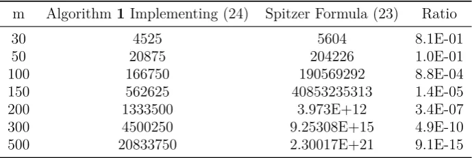
and shows that our method dominates the Spitzer formula for m ≥ 30 and therefore provides greater efficiency in pricing discrete lookback options with a high number of monitoring points. For example, at m = 200, the Spitzer formula (23) requires approximately 9.25×10¹⁵ terms to calculateϕXm compared to 1.33×10
6 using formula (24).
Proposition 4.2Complexity of Formulae (24) and (23): The following statements hold true: a) the Spitzer-recurrence expansion formula(24)is of complexity O(m3), and b) the Spitzer formula
(23) is sub-exponential and requires computation of p(m) individual terms involving ak, where p(m) is the partition function defined as the number of integer partitions of m.
Proof: Provided in Appendix B.2 and B.3.
Table 1. Number of Terms in Evaluating Spitzer Formula (24) and (23)
m Algorithm1 Implementing (24) Spitzer Formula (23) Ratio
30 4525 5604 8.1E-01
50 20875 204226 1.0E-01
100 166750 190569292 8.8E-04
150 562625 40853235313 1.4E-05
200 1333500 3.973E+12 3.4E-07
300 4500250 9.25308E+15 4.9E-10
500 20833750 2.30017E+21 9.1E-15
the strike-separable feature of the pricing formula (17), we are able to price options across multiple strikes in an extremely efficient manner. This is because the spline approximants, ˜s1(t) and ˜s2(t), are independent ofRand are computed only once with the first strike, and the divided differences in (19) can be pre-computed (see Haslip and Kaishev (2013)). Hence the efficiency of the FTBS method for pricing many options simultaneously across a quantum of strike prices is similar to that of pricing a single option.
Algorithm 1Computation ofϕXm(z) using the Spitzer-recurrence expansion formula (24)
Input: m∈N, z∈C Output: ϕXm(z)
for i= 0, . . . , m−1do
P(0, i)← ai(z)
i+1
end for
ϕ←P(0, m−1)
for i= 1, . . . , m−1do for j= 0, . . . , m−1−i do
fork = 0, . . . , j do
P(i, j)←P(i, j) +P(i−1, k)∗P(0, j−k)
end for end for
ϕ←ϕ+P(i,m(i+1)!−1−i)
end for return ϕ
4.2. Calculating ak(z)
We now consider the problem of calculatingak(z) =EQ
(
eizL
+
j∗+k
)
, k = 1, . . . , m, i.e. the charac-teristic function of the greater of the log-return process at timetj∗+k and zero. For simple models of asset log-return, such as Brownian motion, this can be evaluated directly by integrating the probability distribution. For a general semimartingale process, the following theorem applies the Fourier transform to provide a general methodology for calculatingak,k = 1, . . . , m.
Proposition 4.3Fourier Transform Representation ofak(z): IfMLj∗+k(v) =EQ
(
evLj∗+k)exists
by
ak(z) = 1− i 2π
iα+∫ ∞
iα−∞
ϕLj∗+k(−ξ)
z
ξ(ξ+z)dξ, (25)
whereα≥Imz > 12 and k= 1, . . . , m.
Proof: The proof is based on applying the Cauchy residue theorem and the technical details are
therefore omitted.
To evaluate (25), note that it is possible to use either numerical methods, or analytic integration, as illustrated in (26) and (27) of Section 5.1. For example, residue calculus can be used to evaluate (25) in closed-form for some semimartingale processes, as illustrated in Section 5.2, Proposition 5.4 in the case of the VG process. In other cases, the FTBS method may be adapted to efficiently calculate the integral in (25) and hence evaluateak(z) at all required z.
5. Pricing Under Selected Semimartingale Models
In this section, the FTBS method is applied to the problem of pricing discrete lookback options for some popular semimartingale processes. Before we proceed to consider the specifics of individual asset models, we provide a recap of the main algorithm proposed in this paper.
Algorithm 2FTBS Pricing Framework
For a general semimartingale process of the log-return,Lt, the following steps provide the price of a discrete lookback option.
(i) Using Proposition 4.3, derive an analytic formula or an approximation toak(z).
(ii) Apply the Spitzer-recurrence expansion formula in Theorem 4.1 to calculate the charac-teristic functionϕXm(z) of the asset price maximum.
(iii) Fit optimal splines interpolants ˜s1(t) and ˜s2(t) to approximate s1(t) ands2(t) in (7). (iv) Calculate ˜C(T, R) by using Algorithm A1 of Appendix A.3 and use this in (2) or (3) to
price the fixed-strike call or floating put lookback option.
5.1. Brownian Motion and the Merton Jump Diffusion Model
We illustrate Step 1 of the FTBS pricing framework under the Black-Scholes assumptions.
Proposition 5.1Calculation of ak(z) for Brownian motion:
If Lt = σW(t) +µt ∼ N
(
µt, σ2t), where W(t) is standard Brownian motion and µ =r− 12σ2,
σ >0 then
ak(z) = Φ
(
−µ √
tj∗+k σ
)
+1 2e
ztj∗+k(iµ−12zσ 2)
erfc
(
−√ 1
tj∗+k
(
µ
σ +izσ
))
, (26)
where erfc(.) is the complex complimentary error function and k = 1, . . . , m.
Proof: The proof is based on directly integrating with respect to the p.d.f. of the Normal
distribution.
In the following proposition, we show how to apply this approach to the Merton jump diffusion model, as described by Petrella and Kou (2004).
Proposition 5.2Calculation of ak for the Merton Jump Diffusion Model:
If Lt = σW(t) +µt +
∑Nt
i=1Yi, where µ = r − 12σ2 −λζ, ζ = eµJ+
1 2σ
2
J −1, N
t ∼ Po(λ), and Yi ∼N(µJ, σJ2) with σ, σJ, λ >0 then
ak(z) =
∞ ∑ j=0 { Φ (
−µj σj
)
+1 2e
z(iµj−12zσj2)erfc
(
−√1
2
(
µj σj
+izσj
))}
e−λtk(λtj∗+k)
j
j! , (27)
where µj =µtj∗+k +jµJ, σj =
√
jσ2
j +σ2tj∗+k, and erfc(.) is the complex complimentary error
function.
Proof: This follows by conditioning on the number of jumps occurring in [tj∗+1, tj∗+k] under the Poisson distribution. The full derivation is provided in Petrella and Kou (2004).
5.2. The Variance Gamma Process
The VG process can be interpreted as Brownian motion with time changed by an independent Gamma L´evy process. The subordinated time process is often viewed as “business time”, reflecting the random speedups and slowdowns in real-time economic and business activity. We refer the reader to Madan et al. (1998) for a detailed introduction to the VG process, and Kaishev and Dimitrova (2009) for a more recent account on the VG related literature. The risk-neutral dynamics of the log-return process are given byLt =rt+µγt+σW(γt)−ωt, whereW(t) is standard Brownian motion, σ > 0, and γt ∼ Γ
(t
ν, ν
)
with ν > 0. The compensator ω = −ν1ln(1−µν−12σ2ν) is chosen to ensure thatEQ(S(t)) =S(0)ert, and this imposes the requirement that (µ+12σ2)ν <1 on the parameters of the VG process. To calculateak(z), we first need to compute the characteristic functionϕLt(z).
Proposition 5.3 : Let Lt follow a VG process so that Lt = rt+µγt +σW(γt) −ωt, where σ >0, ν >0, and (µ+12σ2)ν <1, under the risk-neutral probability measure. The characteristic
function of Lt is given by
ϕLt(ξ) =e
iξ(r−ω)t
(
1
1−iµνξ+12σ2νξ2
)t
ν
Proof: The proof follows from a result by Madan et al. (1998) for the characteristic function of the real-world log-return process, appropriately extending the domain of the characteristic
function to the complex plain.
To calculate ak(z) for the VG process, we utilize Proposition 4.3 and apply residue calculus to evaluate the contour integral.
Proposition 5.4 : LetLtfollow a VG process, wherer > ωor, equivalently,(µ+12σ2)ν <1−e−rν
is satisfied. Ifs= tj∗+k
ν fork = 1, . . . , m is integer valued then
ak(z) =−2πi[R1(z) +R2(z)], (29)
where
R1(z) = i 2π
(
1−iµνz+1 2σ
2 νz2
)−s
eiz(r−ω)sν (30)
R2(z) = iz
2π(s−1)!
(
1 2σ
2ν)−seiξ2s(r−w)ν
s−1
∑
j1=0
(s+j1−1)!
j1! (ξ2−xi3)
−s−j1
s−∑1−j1
j2=0
(−1)s−1−j2
j2! [is(r−w)v] j2
s−1∑−j1−j2
j3=0
ξ−1−j3
2 (ξ2+z)j1+j2+j3−s, (31)
whereξ1 =−z and ξ2 =−σ2iν (
µν+√µ2ν2+ 2σ2ν). If s is not integer valued for some k, then
we have s = sI +w, where sI = ⌊s⌋ is the integer part of s and w = s−sI, 0 < w < 1.
Then, we estimate ak(z) for a given s as aˆk(z) = −2πi
[
R1(z) + ˆR2(z)
]
, where Rˆ2(z) = (1− w)R2(z)|s=˜sI+wR2(z)|s=˜sI+1.
Proof: The proof utilizes the Cauchy residue theorem to evaluate the integral along the straight lineξ =αias the sum of residues lying below this line and details are therefore omitted.
To avoid computational difficulties with large numbers, we write (31) in terms of logarithms. Additionally, in our implementation we identify a condition on the third summation indexj3 to avoid calculating terms that are smaller than a specified level to improve efficiency. We note that the requirement fors∈Z, whereZ is the set of integers, imposes the restriction that the number of monitoring points,m, should not exceed the time period of the contract (measured in the time units of the VG process calibration). For example, if the calibration is carried out in annual time units, then we are limited to annual monitoring points. However, if half-yearly monitoring points are required, this is achieved by calibrating the VG process to semi-annual time units.
6. Numerical Results
the level of uncertainty around the simulated option price, we repeat the simulation 20 times for each maturity and strike price with ten million simulations at each pricing point. Our unbiased estimator of the option price is the sample mean, and we calculate the standard error of the simulated price to provide an estimate of the simulation error.
In our implementation, we fit optimal splines to boths1(t) ands2(t) in (7) using 200 data points in [0,1]. We allocate the data sites in uniform bands: 60% to [0,0.2), 20% to [0.2,0.6) and the remainder to [0.6,1] (see Haslip and Kaishev (2013) for a further details on this choice of data site allocation). The numerical implementation is in C++, and all computations have been performed using an Intel Core I7-3610QM processor. The complex-valued error function is calculated, as in Petrella and Kou (2004), via the Faddeeva function using an algorithm by Poppe and Wijers (1990), which ensures an accuracy of 13 digits in almost the entire complex plane.
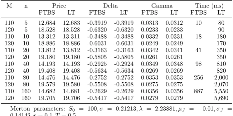
In Table 2 and 3, we provide a comparison of the results under the FTBS method to the LT method of Petrella and Kou (2004), under Brownian motion and the Merton jump diffusion process respectively. We note that Petrella and Kou (2004) use an Intel Pentium 1.8Ghz processor and do not report the software implementation. To illustrate the efficiency of the FTBS method, instead of computing the price of two options for observed asset price maximumM = 110 and M= 120, we price 41 options forM= 101 toM = 140 in steps of one. As described in Section 3.1, the strike-separable pricing formula is extremely efficient for pricing lookback options at a range of different strike prices or observed asset price maximum. Our calculations utilize pre-computation of the required divided differences at the 41 specified asset price maximum levels, as described in Haslip and Kaishev (2013). It should be noted that the divided difference calculation is independent of the choice of the exponential semimartingale process. Therefore, for a fixed set of data sites and corresponding optimal knots, we can pre-compute the divided differences for different values of R and do not need to calculate this each time an option is priced for a different value of R. Furthermore, in our implementation, we use same data sites and knots for the Greeks, and hence the pre-computed divided differences are applied for both pricing and computing the option price sensitivities.
The reported CPU time for the FTBS method is the time taken to calculate all 41 option prices and sensitivities and is compared to the time taken for a single option price and sensitivities under the LT method. We note that our reported CPU times exclude the time taken to pre-compute the required divided differences, but this is a very quick process which took only 60ms in total for the 41 individual options. The FTBS method provides results in very close agreement to the LT method using 200 knots in the optimal interpolation scheme. The FTBS method is faster than the LT method for all choices of the number of monitoring pointsm, and the CPU time of the FTBS is faster by a factor of approximately 5−15 times. The substantial improvement in efficiency for larger m can be explained by the use of the Spitzer-recurrence expansion formula (24) in computing the characteristic function of the asset price maximum. For example, atm= 80, for the Merton jump diffusion model, the FTBS method takes 256ms to price 41 options, whereas the LT method takes 4,070ms to compute two option prices.
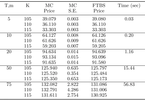
In Table 4, we provide prices for the discrete fixed lookback call option under the VG process for strike prices K = 105, K = 110, and K = 115 for contracts with annual monitoring points and contract duration,T, ranging from 5 to 75 years. Again, the CPU times provided correspond to the total time for computing the price of 40 individual options with strike prices ranging from K = 101 to K = 140 in steps of one. The results show close agreement with the Monte Carlo simulation, and differences are well within one standard deviation of the Monte Carlo results.
Table 2. Pricing Results for Brownian Motion Discrete Floating Lookback Put Option
M n Price Delta Gamma Time (ms)
FTBS LT FTBS LT FTBS LT FTBS LT
110 5 13.300 13.300 -0.3567 -0.3568 0.0288 0.0287 2 20 120 5 18.837 18.837 -0.5924 -0.5924 0.0244 0.0244 10 110 10 14.123 14.123 -0.3032 -0.3034 0.0310 0.0309 4 30 120 10 19.323 19.323 -0.5547 -0.5547 0.0260 0.0260 20 110 20 14.806 14.806 -0.2632 -0.2633 0.0320 0.0319 12 60 120 20 19.743 19.743 -0.5238 -0.5237 0.0272 0.0273 70 110 40 15.345 15.345 -0.2332 -0.2333 0.0324 0.0324 40 190 120 40 20.083 20.083 -0.4998 -0.4999 0.0281 0.0281 190 110 80 15.754 15.754 -0.2111 -0.2112 0.0327 0.0327 145 640 120 80 20.346 20.346 -0.4819 -0.4819 0.0287 0.0287 640 110 160 16.059 16.059 -0.1951 -0.1952 0.0329 0.0329 663 2,340 120 160 20.544 20.544 -0.4687 -0.4687 0.0291 0.0291 2,350
Brownian motion parameters:S0= 100, σ= 0.3, r= 0.1, T = 0.5.
The times (FTBS) are for computing the prices and sensitivities of 41 options, whereas (LT) are the times quoted by Petrella and Kou (2004) are for computing the prices and sensitivities of a single option.
Table 3. Pricing Results for Merton Jump Diffusion Discrete Floating Lookback Put Option
M n Price Delta Gamma Time (ms)
FTBS LT FTBS LT FTBS LT FTBS LT
110 5 12.684 12.683 -0.3919 -0.3919 0.0313 0.0312 10 80 120 5 18.528 18.528 -0.6320 -0.6320 0.0233 0.0233 90 110 10 13.312 13.311 -0.3488 -0.3488 0.0332 0.0331 18 180 120 10 18.886 18.886 -0.6031 -0.6031 0.0249 0.0249 170 110 20 13.812 13.812 -0.3163 -0.3163 0.0342 0.0341 41 350 120 20 19.180 19.180 -0.5805 -0.5805 0.0261 0.0261 350 110 40 14.193 14.193 -0.2925 -0.2924 0.0349 0.0348 98 810 120 40 19.408 19.408 -0.5634 -0.5634 0.0269 0.0269 820 110 80 14.476 14.476 -0.2752 -0.2752 0.0353 0.0353 256 2,000 120 80 19.579 19.580 -0.5508 -0.5508 0.0275 0.0275 2,070 110 160 14.682 14.681 -0.2629 -0.2629 0.0356 0.0356 887 5,550 120 160 19.705 19.706 -0.5417 -0.5417 0.0279 0.0279 5,690
Merton parameters: S0 = 100, σ = 0.21213, λ = 2.23881, µJ = −0.01, σJ = 0.14142, r= 0.1, T = 0.5.
The times (FTBS) are for computing the prices and sensitivities of 41 options, whereas (LT) are the times quoted by Petrella and Kou (2004) are for computing the prices and sensitivities of a single option.
7. Conclusion
[image:20.595.88.462.401.587.2]Table 4. Variance Gamma Option Pricing Results
T,m K MC MC FTBS Time (sec)
Price S.E. Price
5 105 39.079 0.003 39.080 0.03 110 36.110 0.003 36.110
115 33.303 0.003 33.303
10 105 64.127 0.008 64.126 0.20 110 61.626 0.009 61.626
115 59.203 0.007 59.205
20 105 94.634 0.014 94.639 1.16 110 93.134 0.015 93.096
115 91.635 0.014 91.580
50 105 125.940 0.635 125.797 15.44 110 125.520 0.354 125.484
115 125.350 0.653 125.173
75 105 132.082 2.822 131.086 56.83 110 132.791 4.286 131.006
115 131.611 2.754 130.925
S0= 100, µ=−0.2859, σ= 0.1927, ν= 0.25, r= 0.0548.
whose characteristic function satisfies certain regularity constraints. Our novel use of the Peano representation of a divided difference makes the FTBS method extremely efficient. It enables us to evaluate the pricing integral in closed-form once the integrands have been replaced by the B-spline approximants.
Numerical examples have demonstrated the accuracy and efficiency of the FTBS method. Our method also has an important advantage over existing methods for pricing discrete lookback options in that, once the B-spline interpolant has been fitted to the strike-separable function, we are able to price lookback options at a range of different strike prices with virtually no additional computational cost.
Finally, we have given an alternative derivation of the expansion representation of the Spitzer formula due to Wendel (1958), which we call the Spitzer-recurrence expansion formula. This provides a substantial efficiency gain over the Spitzer formula. This is one of the key reasons why our numerical results for the FTBS method have shown such a significant improvement over the Laplace Transform method of Petrella and Kou (2004) for large numbers of monitoring points m. Algorithm 1 which implements the Spitzer-recurrence expansion formula is of fundamental importance since it has many potential applications in wider fields in which the Spitzer formula is employed.
Acknowledgements