©2016 The Authors Journal of the Royal Statistical Society: Series C Applied Statistics Published by John Wiley & Sons Ltd on behalf of the Royal Statistical Society.
This is an open access article under the terms of the Creative Commons Attribution License, which permits use, dis-tribution and reproduction in any medium, provided the original work is properly cited.
0035–9254/17/66141 66,Part1,pp.141–157
An adaptive spatiotemporal smoothing model for
estimating trends and step changes in disease risk
Alastair Rushworth,
University of Strathclyde, Glasgow, UK
Duncan Lee
University of Glasgow, UK
and Christophe Sarran
UK Met Office, Exeter, UK
[Received November 2014. Final revision March 2016]
Summary.Statistical models used to estimate the spatiotemporal pattern in disease risk from areal unit data represent the risk surface for each time period with known covariates and a set of spatially smooth random effects. The latter act as a proxy for unmeasured spatial con-founding, whose spatial structure is often characterized by a spatially smooth evolution between some pairs of adjacent areal units whereas other pairs exhibit large step changes. This spatial heterogeneity is not consistent with existing global smoothing models, in which partial correla-tion exists between all pairs of adjacent spatial random effects. Therefore we propose a novel space–time disease model with an adaptive spatial smoothing specification that can identify step changes. The model is motivated by a new study of respiratory and circulatory disease risk across the set of local authorities in England and is rigorously tested by simulation to assess its efficacy. Results from the England study show that the two diseases have similar spatial patterns in risk and exhibit some common step changes in the unmeasured component of risk between neighbouring local authorities.
Keywords: Adaptive smoothing; Gaussian Markov random fields; Spatiotemporal disease mapping; Step change detection
1. Introduction
Disease risk exhibits spatiotemporal variation due to many factors, including changing lev-els of environmental exposures and risk-inducing behaviours such as smoking. Disease risk data are typically obtained as population level summaries for administrative geographical units, such as local authorities, and the spatial pattern in risk is presented via a choropleth map. Such maps enable public health professionals to quantify the spatial pattern in disease risk, allowing financial resources and public health interventions to be targeted at high-risk areas. Disease maps are routinely published by health agencies world wide, such as the can-cer e-Atlas (http://www.ncin.org.uk/cancer information tools/eatlas/) by Public Health England and the weekly influenza maps (http://www.cdc.gov/flu/ weekly/usmap.htm) that are produced by the Centers for Disease Control and Prevention
Address for correspondence: Alastair Rushworth, Department of Mathematics and Statistics, University of Strathclyde, 26 Richmond Street, Glasgow, G1 1XH, UK.
in the USA. These maps also allow the scale of health inequalities between rich and poor com-munities and their underlying drivers to be quantified. For example, the Office for National Statistics (2014) estimated that UK average healthy life expectancy differs by 19 years between communities with the highest and the lowest levels of deprivation. Such large inequalities exac-erbate socio-economic divisions in society, and health costs may be increased because of higher disease prevalence in the most disadvantaged regions.
Disease maps presented by health agencies display raw disease rates, which do not allow in-ferential statements to be made such as calculating risk exceedence probabilities (Richardson et al., 2004), or evaluating the significance of temporal changes. A range of statistical models have been developed for disease data, which represent the risk surface by using known covari-ates and a set of random effects. The latter act as a proxy for unmeasured spatial confounding and are typically modelled by a Gaussian Markov random-field (GMRF) (Rue and Held, 2005) prior in a hierarchical framework. GMRF priors have been extended to incorporate spatiotem-poral structure, and prominent examples include Bernardinelliet al. (1995), Knorr-Held (2000), MacNab and Dean (2001) and Ugarteet al. (2010).
GMRF models assume that the random effects are globally spatially smooth, in the sense that a single parameter governs the spatial auto-correlation in disease risk between all pairs of geographically adjacent units. In practice, however, this residual or unexplained spatial struc-ture is often characterized by a spatially smooth evolution between some pairs of adjacent units, whereas other pairs exhibit large step changes. The identification of such step changes in the unexplained component of risk is known asWombling, following the seminal article by Womble (1951), and can provide several epidemiological insights. Firstly, it allows the identifica-tion of the geographical extent of clusters of areal units that exhibit elevated unexplained risks, which enables health resources and public health interventions to be targeted appropriately. Secondly, it provides detailed insight into the spatial structure of the unmeasured confound-ing, allowing the identification of unknown aetiological factors that contribute to disease risk. Furthermore, smoothing models that ignore local structure may result in oversmoothing in regions where strong disparities exist and undersmoothing elsewhere, leading to biased esti-mation of disease risk. A range of spatially adaptive smoothing priors have been proposed to address these limitations for purely spatial data, including Green and Richardson (2002), Lu et al. (2007), Lawsonet al. (2012), Lee and Mitchell (2013), Wakefield and Kim (2013) and Lee et al. (2014).
Few spatially adaptive smoothing models have been developed for spatiotemporal disease data, with an exception being Lee and Mitchell (2014) who proposed an iterative fitting al-gorithm using integrated nested Laplace approximations. Although temporal replication is likely to improve the estimation in such highly complex models, the increased numbers of data points and parameters results in much increased computational complexity. Therefore, the contribution of this paper is the development of a computationally feasible spatially adap-tive GMRF model for spatiotemporal disease data, which can be viewed as both an adapadap-tive smoother and a model for the detection of step changes in unexplained risk. The model builds on the purely spatial approach of Ma et al. (2010) and avoids making simplifying assump-tions about the step change structure as Leeet al. (2014) did. Additionally, our model is freely available via the R package CARBayesST(Lee et al., 2015). The methodological develop-ment is motivated by a new study of respiratory and circulatory disease in England, which according to the World Health Organization are two of the largest causes of death world wide
(www.who.int/mediacentre/factsheets/fs310/en/). This study is presented in
tested by simulation in Section 5. In Section 6 the model is applied to the motivating application, and the paper concludes in Section 7.
The data that are analysed in the paper and the programs that were used to analyse them can be obtained from
http://wileyonlinelibrary.com/journal/rss-datasets
2. Motivating case-study
Our methodological development is motivated by a new study of circulatory and respiratory disease risk in England between 2001 and 2010, which have international classification of disease 10th revision codes I00–I99 and J00–J99 respectively. Hospital admissions records from the Health and Social Care Information Centre were analysed at the UK Met Office to provide yearly counts of emergency admissions by local and unitary authorities (LUAs). The resulting data{Yij}are counts of hospital admissions fori=1,: : :,N(N=323) LUAs in England in year
j=1,: : :,T (T=10) and range between 6 and 1030 (circulatory) and 0 and 2485 (respiratory) respectively. The expected numbers of hospital admissions{Eij}were calculated for each year and LUA to adjust for their differing population sizes and demographic structures by using indirect standardization. Specifically, Eij=Σqr=1Nijrpr, where Nijr is the population size in LUAi, yearj and stratumr(e.g. males 0–5), whereaspr is the England-wide risk of disease in stratumr. The expected counts range between 144.8 and 564.1 (circulatory) and 115.2 and 675.9 (respiratory) respectively.
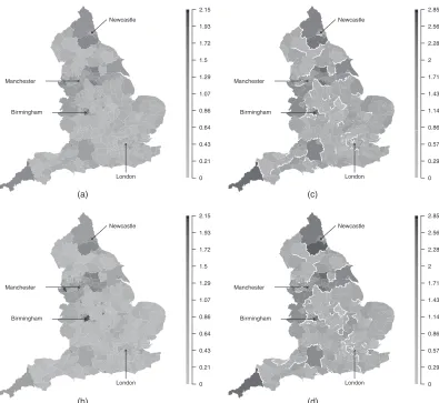
The standardized incidence ratio SIRij=Yij=Eijis an exploratory (noisy) measure of disease risk, and a value of 1.2 corresponds to a 20% increased risk of disease relative toEij. The mean SIR over all years is displayed in Figs 1(a) and 1(b), and similar spatial patterns are evident between the two diseases with a Pearson correlation coefficient of 0.9356. Within each map, the risk levels are spatially smooth across much of England, although several step changes are visible, including around the cities of Birmingham and Manchester. There are various potential drivers of this spatial variation in disease risk, including socio-economic deprivation (poverty), air pollution and the differences between urban and rural areas. We measure poverty by the percentage of the working age population who are in receipt of Jobseeker’s Allowance obtained from the Health and Social Care Information Centre, whereas we obtain modelled particulate matter concentrations PM10 from the Department for Environment, Food and Rural Affairs on a 1-km grid which are then averaged to the LUA scale. Finally, the urban or rural nature of each LUA is measured by the proportion of middle layer super-output areas classified as urban within each LUA. The (mean over year) residuals from a simple Poisson log-linear model with these covariates are displayed in Figs 1(c) and 1(d). The residual unexplained spatial variation in disease risk is auto-correlated for both diseases, with significant (at the 5% level) Moran I-statistics ranging between 0.204 and 0.328 across the years. However, Fig. 1 also highlights that these unexplained spatial structures exhibit step changes, which are not compatible with a global spatial smoothing model.
Newcastle
Birmingham Manchester
Birmingham Manchester
London 0
0.18 0.35 0.52 0.7 0.88 1.05 1.23 1.4 1.58 1.75 –0.7 –0.51 –0.32 –0.13 0.06 0.25 0.44 0.63 0.82 1.01 1.2 –0.7 –0.51 –0.32 –0.13 0.06 0.25 0.44 0.63 0.82 1.01 1.2
Newcastle
Newcastle
Newcastle
Birmingham Manchester
Birmingham Manchester
London London London 0 0.25 0.5 0.75 1 1.25 1.5 1.75 2 2.25 2.5
(a) (c)
[image:4.485.45.442.55.421.2](b) (d)
Fig. 1. Mean standardized incidence ratios for (a) circulatory and (b) respiratory hospital admissions across English local authorities between 2001 and 2010, and mean standardized Pearson residuals from a Poisson log-linear model with Jobseeker’s Allowance, urbanicity and PM10 as covariates for (c) circulatory and (d)
respiratory admissions:!, locations of four major English cities
3. Spatiotemporal disease mapping
The observed and expected disease counts for LUAiand yearj are denoted by.Yij,Eij/ res-pectively, and the following Poisson log-linear model is commonly specified for these data:
Yij|Eij,Rij∼Poisson.EijRij/ i=1,: : :,N, j=1,: : :,T, ln.Rij/=xTijβ+φij,
βr∼N.0, 10000/ r=1,: : :,p:
.1/
Disease risk is represented by Rij, which is on the same scale as the standardized incidence ratio. The log-risk ln.Rij/is modelled by a vector ofpknown covariatesxij=.xij1,: : :,xijp/ with parametersβ=.β1,: : :,βp/, and a spatiotemporal random effectφij. GMRF priors are commonly used to induce spatial smoothness between the random effects, via a binaryN×N adjacency matrixW. Elementwik=1 if areasiandkshare a common border (denotedi∼k) andwik=0 otherwise (denotedik), whereaswii=0 for alli. Numerous GMRF priors have been developed for purely spatial random effects.φ1,: : :,φN/, and the proposal by Lerouxet al. (1999) has an attractive full conditional decomposition given by
φi|φ−i,ρ,τ2,W∼N ⎛ ⎜ ⎜ ⎜ ⎝
ρN k=1wikφk
ρN
k=1wik+1−ρ
, τ
2
ρN
k=1wik+1−ρ ⎞ ⎟ ⎟ ⎟
⎠, .2/
whereφ−i=.φ1,: : :,φi−1,φi+1,: : :,φN/. The conditional expectation ofφiis a weighted aver-age of adjacentφk (as specified byW), which induces smoothness across the surface. Spatial smoothing is controlled byρ∈[0, 1], whereρ=1 corresponds to the intrinsic auto-regressive model (Besag, 1974), whereas ρ=0 corresponds to independence. The resulting joint distri-bution is given by.φ1,: : :,φN/∼N{0,τ2Q.ρ,W/−1}, where the precision matrix is given by Q.ρ,W/=ρ{diag.W1/−W}+.1−ρ/I, where 1is anN×1 vector of 1s andIis theN×N identity matrix.
Many spatiotemporal GMRF models have been developed in the disease mapping literature, with the first being Bernardinelliet al. (1995) who modelledRijwith linear time trends that have spatially varying slopes and intercepts. In contrast, Knorr-Held (2000) introduced a decompo-sition ofRij into spatial and temporal main effects and an interaction, with all terms being modelled by GMRF priors. More recently, Rushworthet al. (2014) utilized the auto-regressive decomposition
f.φ1,: : :,φT/=f.φ1/ T
j=2f.φj|φj−1/, .3/
whereφj=.φ1j,: : :,φNj/. They combined decomposition (3) with the Leroux conditional auto-regressive (CAR) prior for each φj, so that φ1 is modelled by distribution (2), and φj∼ N{αφj−1,τ2Q.ρ,W/−1}forj=2,: : :,T, whereα∈[0, 1] controls temporal auto-correlation. The global nature of the spatial auto-correlation that is induced by distribution (2) for purely spatial random effects.φ1,: : :,φN/can be seen from their theoretical partial auto-correlations:
corr.φi,φk|φ−ik,ρ,W/= ρwik ρN
r=1wir+1−ρ
ρN
s=1wks+1−ρ
Under models (2) and (3), random effects for all pairs of neighbouring areal units (for which wik=1) will be partially auto-correlated, and the strength of that partial auto-correlation will be controlled byρ. Thus, asρwill often be close to 1 (the spatial residual surfaces are auto-correlated as described in Section 2), a pair of adjacent areas exhibiting substantially different levels of unexplained risk will have those risks wrongly smoothed towards each other, masking the step change to be identified. This prompted the development of spatially adaptive smoothing models for spatial data, and the extension to the spatiotemporal domain is one of the contributions of this paper. Brewer and Nolan (2007) and Reich and Hodges (2008) extended GMRF models by allowing the varianceτ2to vary across the study region, whereas Lawsonet al. (2012), Charras-Garridoet al. (2012), Wakefield and Kim (2013) and Andersonet al. (2014) utilized a piecewise constant cluster model in the linear predictor to model step changes between neighbouring areas. Alternatively, Luet al. (2007), Brezgeret al. (2007), Maet al. (2010), Lee and Mitchell (2013) and Leeet al. (2014) generalized CAR models by treating the non-zero elements of the adjacency matrixWas random variables. Under this approach, equation (4) implies that spatially adjacent.φi,φk/can be partially auto-correlated or conditionally independent, depending on the estimated value ofwik.
4. Methodology
4.1. General approach
We present a novel spatially adaptive smoothing model for spatiotemporal data, which allows step changes between adjacent areal units in the unexplained component of risk while treating their locations as unknown. This is achieved by modelling the adjacency elements inW, i.e. w+={wik|i∼k} (of lengthNW=1TW1=2), as random variables on the unit interval, rather than being fixed equal to 1. The remaining elements ofWcorresponding to non-adjacent areal units remain fixed at 0. Equation (4) shows that, whenρis close to 1, then estimatingwik∈w+ as close to 1 results in partial auto-correlation and hence smoothing between the spatially ad-jacent.φij,φkj/for all time periodsj. Conversely, ifwikis estimated as close to 0 then.φij,φkj/ are close to conditionally independent for all time periodsj, and no such spatial smoothing is enforced. In the latter case, a step change is said to exist in the random-effects surface between areal units.i,k/for all time periodsj. We follow Lu and Carlin (2005) and quantify the evidence for a step change by using
pik=P.wik<0:5|Y/, .5/ the posterior probability ofwikbeing less than 0.5. Our proposed model is one of the first adaptive (localized) smoothing models for spatiotemporal data and is outlined in two stages below.
4.2. Level 1—likelihood and random-effects model for (Yij,φij) The first level of our proposed model is given by
Yij|Eij,Rij∼Poisson.EijRij/ i=1,: : :,N, j=1,: : :,T, ln.Rij/=xTijβ+φij,
β0∼N.0, 10000/, φ1∼N{0,τ2Q.W,/−1},
φj|φj−1∼N{αφj−1,τ2Q.W,/−1} j=2,: : :,T, τ2∼inverse-gamma.0:001, 0:001/,
α∼uniform.0, 1/:
The only difference from the model proposed by Rushworthet al. (2014) is that the GMRF prior that was proposed by Lerouxet al. (1999) is replaced by the intrinsic GMRF prior (whereρ=1), which is enforced because attempting to estimateρandWcould result in high posterior correl-ation and multimodality, because the random effects are spatially independent if eitherρ=0 or all elements ofw+equal 0. To avoid rank deficiency of the precision matrix and subsequent problems with matrix inversion, the adjusted specificationQ.W,/=diag.W1/−W+Iis used, whereIis added to ensure thatQ.W,/is diagonally dominant and hence invertible. This in-vertibility condition is required because, in the second level of the model that is described below, elements inWare treated as random variables, necessitating the evaluation of the normalized prior densityf.φj|φj−1/. Sensitivity to the value ofwas checked in an initial modelling step and was found not to affect estimation untilwas increased to a relatively large value, such as >10−2. Therefore in this paper we set=10−7.
4.3. Level 2—adjacency model for elements inwC
Our methodological contribution extends the model of Rushworthet al. (2014) by treating the elements w+ as binary random quantities on the unit interval, rather than being fixed at 1. Specifying a continuous domain forw+allows the direct application of a second-stage GMRF prior, avoiding the need for a discrete prior such as the Ising model, for which no polynomial time algorithm exists to compute its normalizing constant. We modelw+ on the logit scale, v+=log{w+=.1−w+/}, which has the back-transformationw+=exp.v+/={1+exp.v+/}. The GMRF prior that we propose for v+ has a constant mean μ, a constant varianceζ2and a precision matrix defined by the GMRF prior that was proposed by Lerouxet al. (1999). This second-stage GMRF prior requires us to specify an adjacency structure for the elements inv+, and herevik,vrs∈v+are defined as adjacent (denotedik∼rs) if the geographical borders that they represent in the study region share a common vertex. Using this notation, we propose the following GMRF prior forv+:
p.v+|ζ2,ρ,μ/∝exp
−2ζ12
ρ
ik∼rs.vik−vrs/
2+.1−ρ/ vik∈v+
.vik−μ/2
,
ζ2∼inverse-gamma.0:001, 0:001/, ρ∼uniform.0, 1/:
.7/
This form highlights the role of ρ, which controls the extent to which step changes appear spatially clustered around common vertices. Whenρ≈1 the random variablevik, which controls the existence of a step change between areal units.i,k/, is smoothed spatially towards adjacent
vrs via the penaltyΣik∼rs.vik−vrs/2, which thus induces spatially clustered step changes, this model is conceptually similar to the ‘CAR2’ model that was proposed in Maet al. (2010). In contrast, when ρ≈0 eachvik is smoothed non-spatially towards the overall mean μ by the penaltyΣvik∈v+.vik−μ/2, which does not encourage spatial clustering of step changes. To avoid numerical problems when transforming betweenv+andw+, the sample space for eachvik∈v+ is truncated to the interval [−15, 15], yielding a sample space of [0:000000306, 0:999999 7] for wik, which is close to the intended [0, 1] interval.
0.0 0.2 0.4 0.6 0.8 1.0
0.0
0
.2
0.4
0
.6
0.8
1.0
wij
Scaled density
0.0 0.2 0.4 0.6 0.8 1.0
0.0
0
.2
0.4
0
.6
0.8
1
.0
wij
Scaled density
(a)
[image:8.485.117.377.56.510.2](b)
Fig. 2. Scaled prior densities forwijfor prior means (a)μD0 and (b)μD15: ,ζD0:1; ,ζD20; ,ζD100
prior probability in between. The ratio of the densities at {0, 1}depends onζ so, whenζ is small, almost all prior mass is concentrated aroundwik=1, and hence strongly discouraging boundaries. In contrast, asζincreases, the prior becomes more symmetric and ‘U’ shaped, with equal point masses at 0 and 1 expressing ambivalence about the presence or absence of step changes. Thus fixingμ=15 ensures that clear step change decisions, i.e.wikclose to 0 or 1, are preferred over ambiguous values such aswik=0:5.
4.4. Inference
Our model is fitted within a Bayesian framework by using Markov chain Monte Carlo sampling and is freely available via the R packageCARBayesST(Leeet al., 2015). The Markov chain Monte Carlo algorithm is a combination of Gibbs and Metropolis–Hastings steps, and the high dimensionality of the parameter space requires an algorithm that minimizes the overall com-putational burden. We exploit matrix sparsity resulting from the GMRF prior precision matrix wherever possible, using efficient loops written in C++ and matrix triplet form to perform the al-gebraic manipulations. The random effects were updated by using fast one at a time Metropolis– Hastings steps rather than using a joint or block updating scheme. Although joint updates (e.g. Knorr-Held and Rue (2002)) can achieve substantially better mixing for an equivalent number of Markov chain Monte Carlo steps and particularly when the parameters are highly correlated, the computational cost was found to outweigh the benefits of better sampling efficiency. Further details are given in the on-line supporting information accompanying this paper.
5. Simulation study
In this section we comprehensively test the performance of two variants of the proposed model on simulated data under a range of scenarios, and we compare their performance against two commonly used alternatives. The two existing models are those proposed by Knorr-Held (2000) (denoted model 1) and Rushworthet al. (2014) (denoted model 2), although the former is im-plemented with GMRF priors proposed by Lerouxet al. (1999) rather than a convolution of independent and intrinsic GMRF priors. Additionally, model 1 is implemented with indepen-dent interactions (Gaussian with zero mean and a common variance), although three other types of interaction were proposed by Knorr-Held (2000). For more details see the vignette accompanying theCARBayesSTsoftware. Model 3 is the adaptive smoothing model that is proposed here with the simplification thatρ=0, whereas model 4 is the full model whereρis not treated as fixed. Model 3a prioritreats eachwik∈w+independently and therefore does not encourage configurations in which step changes cluster. Our primary focus in this study is to assess the ability of each model to estimate the spatiotemporal pattern in disease risk, and to identify step changes in risk between neighbouring areas.
5.1. Data generation and study design
0.67 0.79 0.9 1.02 1.14 1.26 1.37 1.49 1.61 1.72 1.84
[image:10.485.43.442.55.267.2](a) (b)
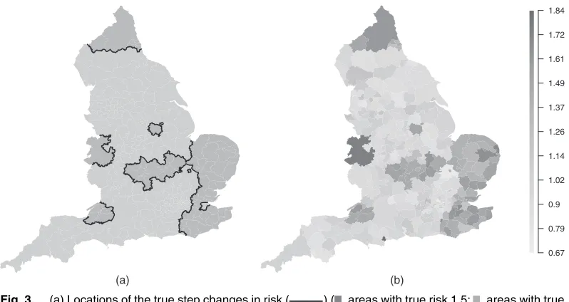
Fig. 3. (a) Locations of the true step changes in risk ( ) ( , areas with true risk 1.5; , areas with true risk 1) and (b) a single realization of the spatial risk surface, assumingAD1.5
Table 1. Description of the scenarios in the simulation study
Scenario type Parameters Parameters
varied fixed
Varying time dimension T∈{1, 5, 20} a=1:5;E=75 Relative risk in high regions A∈{1, 1:5, 2} T=5;E=75 Expected cases E∈{10, 50, 100} T=5;a=1:5
risk level ofA, and the black lines correspond to the locations of true step changes. An example realization of this surface is shown in Fig. 3(b) forA=1:5, where the clusters of high-risk areas are evident. To ensure that the true risk surface is not identical for all time periods, independent random noise is added to the risk in each areal unit for each time period. The scenarios that are considered in this study are summarized in Table 1, which shows that we considerT=1, 5, 20 time periods, elevated risk levels ofA=1, 1:5, 2 and disease prevalences ofE=10, 50, 100. For theA=1 scenario this corresponds to a spatially smooth risk surface with no step changes, which tests the model’s propensity for identifying step changes when none are present (false positive results).
5.2. Results
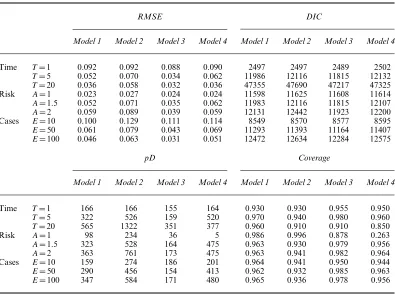
[image:10.485.121.362.310.393.2]Table 2. Median root-mean-squared error RMSE, 95% credible interval coverages associated with the fitted risks, deviance information criterion DIC and the effective number of parameters, pD, for each model and scenario
RMSE DIC
Model 1 Model 2 Model 3 Model 4 Model 1 Model 2 Model 3 Model 4
Time T=1 0.092 0.092 0.088 0.090 2497 2497 2489 2502
T=5 0.052 0.070 0.034 0.062 11986 12116 11815 12132
T=20 0.036 0.058 0.032 0.036 47355 47690 47217 47325 Risk A=1 0.023 0.027 0.024 0.024 11598 11625 11608 11614
A=1:5 0.052 0.071 0.035 0.062 11983 12116 11815 12107
A=2 0.059 0.089 0.039 0.059 12131 12442 11923 12200 Cases E=10 0.100 0.129 0.111 0.114 8549 8570 8577 8595
E=50 0.061 0.079 0.043 0.069 11293 11393 11164 11407
E=100 0.046 0.063 0.031 0.051 12472 12634 12284 12575
pD Coverage
Model 1 Model 2 Model 3 Model 4 Model 1 Model 2 Model 3 Model 4
Time T=1 166 166 155 164 0.930 0.930 0.955 0.950
T=5 322 526 159 520 0.970 0.940 0.980 0.960
T=20 565 1322 351 377 0.960 0.910 0.910 0.850
Risk A=1 98 234 36 5 0.986 0.996 0.878 0.263
A=1:5 323 528 164 475 0.963 0.930 0.979 0.956
A=2 363 761 173 475 0.963 0.941 0.982 0.964
Cases E=10 159 274 186 201 0.964 0.941 0.950 0.944
E=50 290 456 154 413 0.962 0.932 0.985 0.963
E=100 347 584 171 480 0.965 0.936 0.978 0.956
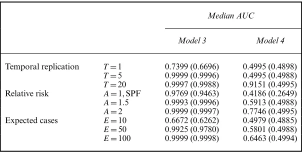
were also computed to quantify the accuracy of the step change detection, which were based on each model’s sensitivity and specificity at identifying true step changes. These statistics compared E[wij|Y] with a threshold valuepÅ, where ifE[wij|Y]< pÅa step change was identified whereas for the converse no step change was declared. The value ofpÅwas varied from 0 to 1 at intervals of 0.01, and the receiver operating characteristic curve is a plot of sensitivity against specificity. However, for ease of presentation the area under the curve, AUC, is presented here rather than the full receiver operating characteristic curve, and AUC=1 corresponds to perfect step change identification. AUC associated with step change estimation was available only for models 3 and 4, as models 1 and 2 do not estimate step changes asw+ is fixed and not estimated in these models. Therefore, AUC is of interest to validate and compare the performance of the adaptive models proposed.
Table 3. Median AUC for step change identification across 100 simulations for models 3 and 4
Median AUC
Model 3 Model 4
Temporal replication T=1 0.7399 (0.6696) 0.4995 (0.4898)
T=5 0.9999 (0.9996) 0.4995 (0.4988)
T=20 0.9997 (0.9988) 0.9151 (0.4995) Relative risk A=1, SPF 0.9769 (0.9463) 0.4186 (0.2649)
A=1:5 0.9993 (0.9996) 0.5913 (0.4988)
A=2 0.9999 (0.9997) 0.7746 (0.4995) Expected cases E=10 0.6672 (0.6262) 0.4979 (0.4885)
E=50 0.9925 (0.9780) 0.5801 (0.4988)
E=100 0.9999 (0.9998) 0.6463 (0.4994)
†Figures in parentheses correspond to the 10% quantile of areas. ForA=1 SPF denotes the specificity since there are no true step changes to identify in this scenario.
3). Overall, Table 2 strongly suggests that the spatial smoothing that is imposed onw+by model 4 is suboptimal compared with assuming that each elementwik∈w+isa priori independent as in model 3. For all models, RMSE decreases as both the number of time periods T and disease prevalenceEincreases, which is due to an increase in the amount of data. Confidence interval coverage was generally very good, with all coverage levels varying between 91% and 97%, except forA=1 when the coverages were 0.986, 0.996, 0.878 and 0.263 for models 1, 2, 3 and 4 respectively.
Table 3 displays the median AUC-statistic across the set of receiver operating characteristic curves calculated for each scenario. The numbers in parentheses are the 10th percentile of that distribution and summarize the variation across the 100 simulated data sets. An exception to this is theA=1 scenario, which displays the specificity because as the risk surface is spatially smooth there are no true step changes to identify. For model 3 the median AUC-values are close to the maximal value of 1, indicating very accurate step change identification. The exceptions to this occur whenT=1 (AUC=0.7399) andE=10 (AUC=0.6672), which result from limited information about step change location provided by the data in both cases. In contrast, model 4 always performs much less well, with median AUC-values ranging between 0.42 and 0.9151. The poor performance of model 4 is also evident in the 10th percentile results, and reinforces the RMSE- and coverage results that are displayed in Table 2. It is likely to be because model 4 forces the step changes to be spatially smooth, thus inducing a set of false positive results that are spatially close to the real boundaries. The other main result from Table 3 is that AUC increases as the number of time periodsTincreases and as the size of the expected cases increases, which is because of an increase in the amount of data.
6. Results of the England case-study
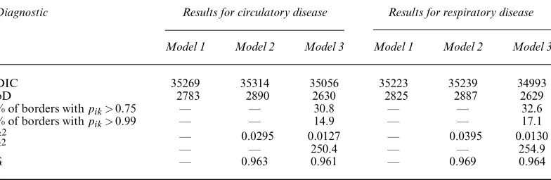
Table 4. Diagnostics for models 1–3 for the England circulatory and respiratory admissions data sets
Diagnostic Results for circulatory disease Results for respiratory disease
Model 1 Model 2 Model 3 Model 1 Model 2 Model 3
DIC 35269 35314 35056 35223 35239 34993
pD 2783 2890 2630 2825 2887 2629
% of borders withpik>0:75 — — 30.8 — — 32.6 % of borders withpik>0:99 — — 14.9 — — 17.1
ˆ
τ2 — 0.0295 0.0127 — 0.0395 0.0130
ˆ
ζ2 — — 250.4 — — 254.9
ˆ
α — 0.963 0.961 — 0.969 0.964
Rushworthet al. (2014) (model 2) and the adaptive smoothing model that is proposed here with the simplification thatρ=0 (model 3). The three covariates that were discussed in Section 2 are included in each model, which are the proportion of working age people claiming Jobseeker’s Allowance, the proportion of each LUA classified as urban, urbanicity, and the particulate matter concentrations PM10. Inference for all models is based on thinning (by 10) 106posterior samples including a burn-in period of a further 105samples. In analysing these data our goals are
(a) to estimate the spatiotemporal pattern in disease risk to quantify the extent of health inequalities and
(b) to estimate the location of any step changes in the unexplained spatial risk structure, which will assist in the identification of unmeasured confounders.
The analysis that is provided here can be reproduced by using the code and data that are available from
http://wileyonlinelibrary.com/journal/rss-datasets
6.1. Model fit
The top two rows of Table 4 display the overall fit of each model to each data set, by presenting DIC and the effective number of parameters pD. It shows that the adaptive smoothing model 3 fits the data better than the global smoothing models 1 and 2 for both diseases, with reductions in DIC in both cases. Additionally, model 3 has a markedly smaller number of effective parameters pD than models 1 and 2, despite having a more complex specification. This is because its ability to identify step changes permits the GMRF component to smooth more strongly elsewhere in the spatial surface, resulting in smaller variance estimates forτ2than from model 2. This implies a greater level of penalization of the random effects and hence a reduction in the overall pD.
6.2. Covariate effects
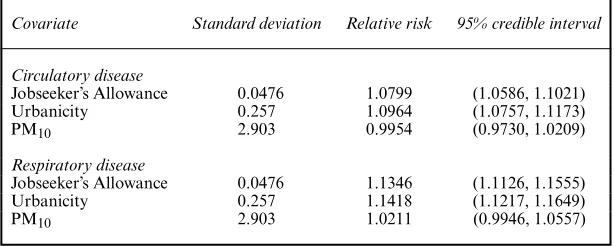
Table 5. Relative risks and associated 95% credible intervals associated with 1-standard-deviation increases in each covariate, as estimated by model 3
Covariate Standard deviation Relative risk 95% credible interval
Circulatory disease
Jobseeker’s Allowance 0.0476 1.0799 (1.0586, 1.1021) Urbanicity 0.257 1.0964 (1.0757, 1.1173)
PM10 2.903 0.9954 (0.9730, 1.0209)
Respiratory disease
Jobseeker’s Allowance 0.0476 1.1346 (1.1126, 1.1555) Urbanicity 0.257 1.1418 (1.1217, 1.1649)
PM10 2.903 1.0211 (0.9946, 1.0557)
for differences in average lifestyle such as prevalence of smoking, drinking and exercise. Both diseases also show substantial effects of urbanicity on disease risk, with more urban areas exhibiting increased risks of 1.096 (circulatory) and 1.142 (respiratory) respectively. Finally, particulate matter air pollution appears to have no effect on circulatory disease risk and a slight effect on respiratory disease risk, with the latter relative risk being 1.021.
6.3. Health inequalities
Maps of the average risks across all years from model 3 are displayed in Figs 4(a) and 4(b) and show similar spatial patterns in risk for both diseases, with a Pearson correlation coefficient of 0.892. The maps show that the average risk varies over space with values between 0.433 and 1.636, and 0.175 and 2.147 respectively for circulatory and respiratory disease, suggesting the presence of substantial health inequalities. These inequalities have generally widened over time, as the difference between the highest and lowest respiratory disease risk was 1.77 in 2001 and 2.13 in 2010. For circulatory disease a similar pattern is evident, with an estimated difference between highest and lowest risk of 1.39 in 2001 and 1.54 in 2010.
6.4. Step change identification
Table 4 summarizes the number of step changes in the unexplained component of the risk surface, based onpik=P.wik<0:5|Y/values above a threshold of 0.75 and 0.99. The higher 0.99-level threshold was used by Lu and Carlin (2005) and results in 15.1% of borders being step changes for circulatory disease and 17.1% for respiratory disease. These step changes are largely similar between the diseases, with 92% agreement between their locations. They are displayed in Figs 4(a) and 4(b) as white lines, whereas the grey shading represents the time-averaged exponentiated random-effects surface which corresponds to the unexplained component of the variation in disease risk. Fig. 4 shows evidence of much higher unexplained risks of hospital admission in areal units containing large cities, and in the central band of northern England that incorporates Manchester and Yorkshire, even after adjusting for the covariates. It is striking that these features are largely consistent between the two diseases so, although the estimated risks have different overall magnitudes, they exhibit very similar spatial patterns. Public health professionals can use these results to identify potential risk factors for disease, by searching for risk factors that exhibit step changes in the same locations as those exhibited in Fig. 4.
6.5. Sensitivity analysis
Newcastle
Birmingham Manchester
London 0 0.21 0.43 0.64 0.86 1.07 1.29 1.5 1.72 1.93 2.15
Newcastle
Birmingham Manchester
London 0 0.29 0.57 0.86 1.14 1.43 1.71 2 2.28 2.56 2.85
Newcastle
Birmingham Manchester
London 0 0.21 0.43 0.64 0.86 1.07 1.29 1.5 1.72 1.93 2.15
Newcastle
Birmingham Manchester
London 0 0.29 0.57 0.86 1.14 1.43 1.71 2 2.28 2.56 2.85
(a)
(b)
(c)
[image:15.485.49.444.53.416.2](d)
Fig. 4. Maps showing (a), (b) the average risk surface and (c), (d) the unexplained component of the risk surface for (a), (c) circulatory disease and (b), (d) respiratory disease: , step changes that have been identified by using a cut-off ofpik0:99 in model 5
in prior specifications. In particular, the shape and scale parameters in the hyperpriors forζ2 andτ2were changed to (1, 1) and (1, 0.001), and the prior variance forβwas reduced to 100. The results that were reported above were found to be robust to these modifications. Our choice of inverse gamma priors here is due to their conjugacy, but alternatives could be explored such as the half-Cauchy distribution as suggested by Gelman (2006).
7. Discussion
the class of GMRF prior distributions and is one of the first models for step change identification in spatiotemporal disease risk. Freely available software via theCARBayesSTpackage for R is provided to allow others to utilize our model, and this is one of the first R packages for spatiotemporal areal unit modelling.
The simulation study in Section 5 established the superiority of our model over global smooth-ing alternatives, in terms of both risk estimation and model fit. Our model was successful at recovering the locations of known step changes in simulated data, with AUC-statistics close to 1 for a range of scenarios. These AUC-statistics were higher if the step changes were assumed to be independent in space, becausea prioriassuming spatial clustering resulted in false step changes being identified close to real step changes. This is an interesting result, as one may have naively assumed that for spatial data the step changes should be modelled spatially, which we have shown is not so. Thus existing global smoothing models are suboptimal for space–time disease mapping in two respects: they smooth over such step changes leading to poorer estimation of disease risk, and they cannot identify such step changes which themselves provide aetiological evidence about potential unmeasured risk factors.
Section 6 provided strong evidence of step changes in the unexplained component of risk for the England data. Additionally, better model fit with a smaller number of effective parameters was observed compared with the global smoothing models, due to increased levels of smoothing in locations where step changes were absent. Thus non-adaptive smoothing models may overfit some data sets, by imposing too weak a spatial smoothing constraint because of step changes in risk. A striking association was found between the fitted risks and identified step changes between circulatory and respiratory disease, perhaps indicating the influence of the same unobserved risk factors. Therefore in future work we shall try to identify such unmeasured confounders, to see whether they are indeed common to both diseases. A univariate approach to modelling was taken here as discussed in Section 2, but the between-disease correlation naturally suggests a bivariate spatiotemporal model as a future avenue of work. Such models have yet to be proposed in a spatiotemporal context and would require the extension of multivariate spatial models such as multivariate CAR (Gelfand and Vounatsou, 2003) models and shared component models (Knorr-Held and Best, 2001). A final avenue for future work is to use the model in an ecological regression context, where the effect of an exposure on disease risk is of primary interest rather than the spatiotemporal pattern in disease risk. The efficacy of adaptive smoothing models in this context may be to reduce spatial confounding between the random effects and the covariates as suggested by Claytonet al. (1993), due to the reduction in the random-effects variance (see Table 4), and environmental factors such as air pollution would be a natural context for such work.
Acknowledgements
This work was funded by the Engineering and Physical Sciences Research Council, via grant EP/J017442/1, and the authors thank the Associate Editor and a reviewer for their constructive comments that greatly improved the paper.
References
Anderson, C., Lee, D. and Dean, N. (2014) Identifying clusters in Bayesian disease mapping.Biostatistics,15, 457–469.
Bernardinelli, L., Clayton, D., Pascutto, C., Montomoli, C., Ghislandi, M. and Songini, M. (1995) Bayesian analysis of space-time variation in disease risk.Statist. Med.,14, 2433–2443.
Besag, J., York, J. and Molli´e, A. (1991) Bayesian image restoration, with two applications in spatial statistics. Ann. Inst. Statist. Math.,43, 1–20.
Brewer, M. J. and Nolan, A. J. (2007) Variable smoothing in Bayesian intrinsic autoregressions.Environmetrics,
18, 841–857.
Brezger, A., Fahrmeir, L. and Hennerfeind, A. (2007) Adaptive Gaussian Markov random fields with applications in human brain mapping.Appl. Statist.,56, 327–345.
Charras-Garrido, M., Abrial, D., De Go¨er, J., Dachian, S. and Peyrard, N. (2012) Classification method for disease risk mapping based on discrete hidden Markov random fields.Biostatistics,13, 241–255.
Clayton, D., Bernardinelli, L. and Montomoli, C. (1993) Spatial correlation in ecological analysis.Int. J. Epidem.,
22, 1193–1202.
Gelfand, A. E. and Vounatsou, P. (2003) Proper multivariate conditional autoregressive models for spatial data analysis.Biostatistics,4, 11–15.
Gelman, A. (2006) Prior distributions for variance parameters in hierarchical models (comment on article by Browne and Draper).Baysn Anal.,1, 515–534.
Green, P. J. and Richardson, S. (2002) Hidden Markov models and disease mapping.J. Am. Statist. Ass.,97, 1055–1070.
Knorr-Held, L. (2000) Bayesian modelling of inseparable space-time variation in disease risk.Statist. Med.,19, 2555–2567.
Knorr-Held, L. and Best, N. G. (2001) A shared component model for detecting joint and selective clustering of two diseases.J. R. Statist. Soc.A,164, 73–85.
Knorr-Held, L. and Rue, H. (2002) On block updating in Markov random field models for disease mapping. Scand. J. Statist.,29, 597–614.
Lawson, A. B., Choi, J., Cai, B., Hossain, M., Kirby, R. S. and Liu, J. (2012) Bayesian 2-stage space-time mixture modeling with spatial misalignment of the exposure in small area health data.J. Agric. Biol. Environ. Statist.,
17, 417–441.
Lee, D. and Mitchell, R. (2013) Locally adaptive spatial smoothing using conditional auto-regressive models. Appl. Statist.,62, 593–608.
Lee, D. and Mitchell, R. (2014) Controlling for localised spatio-temporal autocorrelation in long-term air pollution and health studies.Statist. Meth. Med. Res.,23, 488–506.
Lee, D., Rushworth, A. and Napier, G. (2015) CARBayesST: spatio-temporal generalised linear mixed models for areal unit data.R Package Version 2.1. University of Strathclyde, Glasgow.
Lee, D., Rushworth, A. and Sahu, S. K. (2014) A Bayesian localized conditional autoregressive model for esti-mating the health effects of air pollution.Biometrics,70, 419–429.
Leroux, B. G., Lei, X. and Breslow, N. (1999) Estimation of disease rates in small areas: a new mixed model for spatial dependence. InStatistical Models in Epidemiology, the Environment, and Clinical Trials, pp. 179–191. New York: Springer.
Lu, H. and Carlin, B. P. (2005) Bayesian areal wombling for geographical boundary analysis.Geog. Anal.,37, 265–285.
Lu, H., Reilly, C. S., Banerjee, S. and Carlin, B. P. (2007) Bayesian areal wombling via adjacency modeling. Environ. Ecol. Statist.,14, 433–452.
Ma, H., Carlin, B. P. and Banerjee, S. (2010) Hierarchical and joint site-edge methods for medicare hospice service region boundary analysis.Biometrics,66, 355–364.
MacNab, Y. C. and Dean, C. (2001) Autoregressive spatial smoothing and temporal spline smoothing for mapping rates.Biometrics,57, 949–956.
Office for National Statistics (2014) Inequality in healthy life expectancy at birth by national deciles of area deprivation: England, 2009-11. Office for National Statistics, Newport.
Reich, B. J. and Hodges, J. S. (2008) Modeling longitudinal spatial periodontal data: a spatially adaptive model with tools for specifying priors and checking fit.Biometrics,64, 790–799.
Richardson, S., Thomson, A., Best, N. and Elliott, P. (2004) Interpreting posterior relative risk estimates in disease mapping studies.Environ. Hlth Perspect.,112, 1016–1025.
Rue, H. and Held, L. (2005)Gaussian Markov Random Fields: Theory and Applications. Boca Raton: CRC Press. Rushworth, A., Lee, D. and Mitchell, R. (2014) A spatio-temporal model for estimating the long-term effects of
air pollution on respiratory hospital admissions in Greater London.Spatl Spatio-temp. Epidem.,10, 29–38. Ugarte, M. D., Goicoa, T. and Militino, A. F. (2010) Spatio-temporal modeling of mortality risks using penalized
splines.Environmetrics,21, 270–289.
Wakefield, J. and Kim, A. (2013) A Bayesian model for cluster detection.Biostatistics,14, 752–765. Womble, W. (1951) Differential systematics.Science,114, 315–322.
Supporting information
Additional ‘supporting information’ may be found in the on-line version of this article: