City, University of London Institutional Repository
Citation
:
Paraskevopoulos, D. C., Bektaş, T., Crainic, T. G. & Potts, C. N. (2016). A cycle-based evolutionary algorithm for the fixed-charge capacitated multi-commodity network design problem. European Journal of Operational Research, 253(2), pp. 265-279. doi: 10.1016/j.ejor.2015.12.051This is the draft version of the paper.
This version of the publication may differ from the final published
version.
Permanent repository link:
http://openaccess.city.ac.uk/19844/Link to published version
:
http://dx.doi.org/10.1016/j.ejor.2015.12.051Copyright and reuse:
City Research Online aims to make research
outputs of City, University of London available to a wider audience.
Copyright and Moral Rights remain with the author(s) and/or copyright
holders. URLs from City Research Online may be freely distributed and
linked to.
City Research Online: http://openaccess.city.ac.uk/ [email protected]
A cycle-based evolutionary algorithm for the fixed-charge
capacitated multi-commodity network design problem
Dimitris C. Paraskevopoulos
School of Management, University of Bath, Claverton Down, Bath, BA2 7AY, UK
Tolga Bekta¸s
Southampton Business School, Centre for Operational Research, Management Science and Information Systems (CORMSIS), University of Southampton, Southampton, SO17 1BJ,
UK
Teodor Gabriel Crainic
D´epartement Management et Technologie, ´Ecole des Sciences de la Gestion, Interuniversity Research Centre on Enterprise Networks, Logistics and Transportation (CIRRELT), Universit´e du Qu´ebec `a Montr´eal, C.P. 8888, succ. Centre-ville, Montr´eal
QC Canada H3C 3P8
Chris N. Potts
Mathematical Sciences, CORMSIS, University of Southampton, Southampton, SO17 1BJ, UK
Abstract
This paper presents an evolutionary algorithm for the fixed-charge multi-commodity network design problem (MCNDP), which concerns routing mul-tiple commodities from origins to destinations by designing a network through selecting arcs, with an objective of minimizing the fixed costs of the selected arcs plus the variable costs of the flows on each arc. The proposed algorithm evolves a pool of solutions using principles of scatter search, interlinked with an iterated local search as an improvement method. New cycle-based neigh-bourhood operators are presented which enable complete or partial re-routing of multiple commodities. An efficient perturbation strategy, inspired by ejec-tion chains, is introduced to perform local compound cycle-based moves to explore different parts of the solution space. The algorithm also allows infea-sible solutions violating arc capacities while forming the “ejection cycles”, and subsequently restores feasibility by systematically applying correction moves.
Email addresses: [email protected](Dimitris C. Paraskevopoulos),
Computational experiments on benchmark MCNDP instances show that the proposed solution method consistently produces high-quality solutions in rea-sonable computational times.
Keywords: multi-commodity network design, scatter search, evolutionary algorithms, ejection chains, iterated local search
1. Introduction
The fixed-charge capacitated multi-commodity network design problem (MCNDP) consists of designing a network on a given graph by selecting arcs to route a given set of commodities between origin-destination pairs. Each arc has a predefined capacity specifying the maximum flow that the arc can accommodate. Also, associated with each arc are fixed and variable costs, where the fixed cost is incurred only if the arc is selected, and the variable cost is a cost per unit of flow along the arc. Each commodity has an origin and a destination node and the amount to be transported. The objective is to minimize the total cost of establishing the arcs and routing the flows.
results of computational experiments conducted on benchmark instances us-ing an algorithm incorporatus-ing the various elements described above. The majority of the heuristics for the MCNDP utilize a trajectory-based or an evolutionary framework to select arcs for inclusion in the design, and subse-quently call a commercial optimizer (e.g., CPLEX) to solve the corresponding flow subproblem. As the flow subproblems become larger, the solution time for repeatedly finding minimum cost flows might become significant, even though linear programming optimizers are relatively efficient. Towards this end, we call the linear programming (LP) solver as few times as possible in the proposed algorithm in order to reduce its computational requirements.
The remainder of this paper is organized as follows. Section 2 provides a brief review of the recent literature on the MCNDP. Section 3 presents our evolutionary algorithm and all of its components, namely the initialization phase, the SS, and the ILS. In Section 4, we describe details of our compu-tational experiments, and we also present results of applying the proposed algorithm to benchmark MCNDP instances from the literature. Conclusions are given in Section 5, where future research directions are also presented.
2. Literature
A number of efficient algorithms have appeared in the literature to address the inherent complexity of solving the MCNDP. In this section, we provide a brief review of the available methods but focus on heuristic, as opposed to exact, solution algorithms for reasons stated earlier.
Crainic et al. (2000) propose a simplex-based tabu search method for the MCNDP using a path-flow based formulation of the problem. Their method combines column generation with pivot-like moves of single commodity flows to define the path flow variables. In a similar fashion, Ghamlouche et al. (2003) describe cycle-based neighbourhoods for use in metaheuristics aimed at solv-ing MCNDPs. The main idea of the cycle-based local moves is to redirect commodity flows around cycles in order to remove existing arcs from the net-work and replace them with new arcs. They use the proposed neighbourhood structures in a tabu search algorithm, where a commodity flow subproblem is solved to optimality at each iteration.
GRASP, originally proposed by Feo and Resende (1995), to produce a diversi-fied initial set of solutions. Each commodity path is subject to an improvement process. The solutions are combined by choosing the best path for each com-modity among the solutions that are being combined. A feasibility restoration mechanism is also available for solutions that are infeasible. In contrast to the recombination process of Alvarez et al. (2005), our SS does not consider commodity paths to build a solution; instead, independent arcs are combined to create offspring. We believe that the latter enhances the SS algorithm’s capabilities, as more combinations can occur when arcs instead of paths are combined together, leading to a rich pool of offspring.
A parallel cooperative strategy is described by Crainic and Gendreau (2002) using tabu search and various communication strategies. In a simi-lar fashion, Crainic et al. (2006) propose a multilevel cooperative search on the basis of local interactions among cooperative searches and controlled in-formation gathering and diffusion. The focus of their algorithm is on the specification of the problem instance solved at each level and the definition of the cooperation operators.
Katayama et al. (2009) propose a column and row generation heuristic for solving the MCNDP. The authors relax the arcs’ capacity constraints, while a column and row generation technique is developed to solve the relaxed prob-lem. Using similar ideas, Yaghini et al. (2013) present a hybrid simulated annealing (SA) and column generation (CG) algorithm for solving the MC-NDP. The SA is used to define the open and closed arcs, wherein the flow subproblem is solved via CG.
A local branching technique for the MCNDP is proposed by
Rodr´ıguez-Mart´ın and Salazar-Gonz´alez (2010). Even though the method, originally
pro-posed by Fischetti and Lodi (2003), is exact by nature, high quality heuristic solutions can be produced using an MIP solver as a “black box”. A solution framework that employs a combination of mathematical programming algo-rithms and heuristic search techniques is introduced by Hewitt et al. (2010). Their methodology uses very large neighbourhood search in combination with an IP solver on an arc-based formulation of the MCNDP, and a linear program-ming relaxation of the path-based formulation using cuts discovered during the neighbourhood search. A follow-up study by Hewitt et al. (2012) intro-duces a generic branch-and-price guided algorithm for integer programs with an application to the MCNDP.
3. Solution Methodology
detail the components of the main algorithm.
3.1. Problem definition
The MCNDP is defined on a graph G = (N,A), where N is the set of
nodes and A is the set of arcs. Each arc (i, j) ∈ A has an associated fixed
cost fij that is incurred if it is selected for inclusion in the network, has a cost
per unit of flow cij, and has a capacity uij. A set of commodities denoted by
P is given, where each commodity has an origin, a destination, and a quantity
to be shipped from origin to destination. Problems with more than one origin or destination per commodity can be modelled by splitting commodities (see Holmberg and Yuan, 2000).
The goal of the problem is to select a subset of arcs that are to be included in the final design of the network along with the commodity flows on these arcs, to minimize the total cost of the selected arcs and the flow distribution on the resulting network. For simplicity, we will refer to the arcs that are included
in the final design of the network as open arcs; otherwise, the arcs should be
considered as closed. Binary variables yij are used, where yij = 1 if the arc
(i, j)∈ A is open, and yij = 0 otherwise. The flow on each arc (i, j)∈ A that
is used for shipping each commodity p ∈ P from its origin to its destination
is denoted by xpij. Conservation of flow constraints must be satisfied at each
node, and there are capacity constraints of the form ∑p∈Pxpij ≤ uij for each
(i, j) ∈ A. The cost f(s) of a solution s that is defined by variables xpij and
yij for (i, j)∈ A and p∈ P is computed using
f(s) = ∑
(i,j)∈A
∑
p∈P
cijx p ij +
∑
(i,j)∈A
fijyij. (1)
We adopt the convention that f(s) =∞ if solution s is infeasible.
Two types of mathematical formulations for the problem appear in the literature; an arc-based and a path-based formulation. We refer to Gendron et al. (1998), Frangioni and Gendron (2001) and Hewitt et al. (2010) for details of these mathematical formulations.
3.2. Evolutionary algorithm
Our proposed solution methodology is an evolutionary algorithm that evolves a population of solutions using the principles of SS and applies ILS (Louren¸co et al., 2002) as an improvement method. Following the basic tem-plate of the SS framework, our solution approach is composed of three distinct
phases: (i) anInitialization phase where a population of good and diverse
so-lutions is produced and a Reference Set (set R) is initialized; (ii) a Scatter
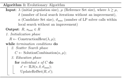
and (iii) an Education phase where these offspring (hosted in set C) are “ed-ucated” by attempting to improve their quality via the proposed ILS. Com-putational time is used as the termination criterion. The framework is given in Algorithm 1.
Algorithm 1: Evolutionary Algorithm
Input: λ (initial population size), µ (Reference Set size), whereλ≥µ,
δ (number of local search iterations without an improvement),
κ (Candidate Set size), ϑmax (number of LP solver calls within
local search without an improvement)
Output: R, sbest ∈R 1. Initialization phase
R ←ConstructionHeur(λ, µ);
while termination conditions do 2. Scatter Search phase
C ← SolutionCombination(κ, µ);
3. Education phase
for individual s of C do
s′ ← ILS(s, δ, ϑmax);
[image:7.595.100.497.145.400.2]UpdateRefSet(R, s′);
Figure 1 illustrates the proposed evolutionary algorithm in a flow chart, the different components making up different process steps, as they are described in the following. The Scatter Search is composed of the Solution Combination method and the pool of offspring, while the Iterted Local Search (described in Section 3.6) consists of the Local Search and the Ejection Cycles. Evaluation of the solutions is performed by the Reference Set Update rationale (described in Section 3.5.1).
Figure 1: A flow chart of the proposed Evolutionary Algorithm
[image:7.595.129.471.555.673.2]below. Prior to this, however, we describe a flow routing procedure that is used in each phase of our algorithm.
3.3. Routing/re-routing procedure
In the Initialization phase of Algorithm 1, solutions are created by suc-cessively adding flow to an existing partial solution by selecting a commodity and routing its required flow from origin to destination. A similar solution creation method is used in some iterations of the Scatter Search phase where some open arcs are selected by the solution recombination method but more are needed to create a feasible flow. Finally, when applying Iterated Local Search within the Education phase, re-routing of flow is applied both in the process for creating neighbours of the current solution and in the procedure for perturbing the current solution. In each of these phases, the routing or re-routing is determined from the solution of a shortest path problem that is obtained by applying Dijkstra’s algorithm. We now provide details of how these shortest path problems are defined.
Consider a partial solution defined by yij = ¯yij and xpij = ¯x
p
ij for each arc
(i, j)∈ A and each commodity p∈ P. Thus, ¯yij = 1 for each arc (i, j) that is
open in the partial solution, uij −
∑
p∈Px¯ p
ij is the remaining capacity in each
arc (i, j). The aim is to route wp units of flow of some commodity p from
node ip to node jp, for appropriately defined wp and nodesip and jp.
There are two alternative shortest path problems that we define. For a
single-path routing, a path from ip to jp is required such that each of arc of
the path has a remaining capacity of at least wp, thereby allowing all of the
desired wp units of flow to be routed along this path. On the other hand, for
multiple-path routing, it is sufficient to find a path where each of its arcs has a non-zero remaining capacity. For both types of routing, we define a shortest
path problem on the original graph G with a cost ¯cij for each arc (i, j) ∈ A,
for suitably defined values of ¯cij.
For single-path routing, we define for each arc (i, j)∈ A
¯
cij =
{
wpcij +fij(1−y¯ij) if wp ≤uij −
∑
p∈Px¯ p ij,
∞ otherwise.
Thus, only arcs that can accommodate an additional wp units of flow have a
finite cost. For an arc (i, j) that can accommodate this additional flow, ¯cij is
the cost of that flow in arc (i, j) plus any additional cost of opening arc (i, j)
if it is not already open in the current partial solution.
For multiple-path routing, we similarly define for each arc (i, j)∈ A
¯
cij =
{
min{uij−
∑
p∈Px¯ p
ij, wp}cij +fij(1−y¯ij) if
∑
p∈Px¯ p
ij < uij,
In this case, arc (i, j) can be used for an additional min{uij −
∑
p∈Px¯ p ij, wp}
units of flow. If this value is strictly positive, then ¯cij is the is the cost of that
flow in arc (i, j) plus any additional cost of opening arc (i, j); otherwise, arc
(i, j) cannot accommodate any additional flow and therefore the value of ¯cij
is set to infinity.
For both types of routing, Dijkstra’s algorithm is applied to find the
short-est path from nodeip to nodejp. If the shortest path length is not finite, then
no routing of flow is possible. Otherwise, in the case of single-path routing, a
flow augmentation process addswp units of flow to all arcs of the shortest path
from node ip to nodejp. Analogously, in the case of multiple-path routing, if
P is the shortest path fromip tojp, then min{min
(i,j)∈P{uij−
∑
p∈Px¯ p
ij}, wp}
units of flow are added to all arcs of P.
3.4. Initialization phase
In the Initialization phase, each iteration of the construction heuristic
se-lects an unrouted or partially routed commoditypat random. Then, a random
choice is made as to whether a single-path or multiple-path routing is to be attempted with an equal probability for each choice.
For a single-path routing,wp is amount of flow for commodityp that is to
be routed, andip and jp are the origin and destinations nodes for this flow. If
the shortest path computation, as described in Section 3.3, provides a solution with a finite shortest path length, then the flow is augmented. After removing
commodity p from the set of unrouted or partially routed commodities and
updating the variables ¯yij and ¯xpij, the heuristic proceeds to the next iteration.
Otherwise, no single-path routing of the chosen commodity exists, and this iteration is repeated using multiple-path routing.
For a multiple-path routing,wp,ip andjp are defined as above. Following
the shortest path computation described in Section 3.3, the flow is augmented
and the values of ¯wp, ¯yij and ¯xpij are updated (with commodity p removed
from the list of unrouted or partially routed commodities if wp is reduced to
zero), and the heuristic proceeds to the next iteration.
The construction heuristic is applied repeatedly untilλ different solutions
are created, among which µ are selected to build the Reference Set. Details
about the creation of the initial Reference Set are given in Section 3.5.1.
3.5. Scatter Search
The SS phase evolves the Reference Set of solutions using an efficient
recombination method as follows. A subset generation method selects κ
so-lutions from the Reference Set, which form the Candidate Set (CS), and a solution combination method is then applied to produce one solution. This
number of parent solutions in the Reference Set. We choose µbest solutions,
in terms of the solution cost, out of the 2µ offspring to proceed to the next
phase. Other strategies were also tested, such as randomly choosing µ of 2µ
solutions, but the algorithm performs better by choosing µ best solutions.
The offspring are checked as to whether they meet the criteria to be inserted into the Reference Set or not, before proceeding to the Education phase. In the Education phase, ILS is used to improve the quality of each offspring, before these offspring are checked again for insertion into the Reference Set according to elitist criteria. These procedures are explained further in the following subsections.
3.5.1. Reference Set
The goal of using a Reference Set R is to maintain a balance between
quality and diversity of solutions, and to avoid a premature convergence of
the algorithm. An obvious measure of the quality of a solutionsis its costf(s).
An alternative quality measure that becomes relevant after the evolutionary
process has started is the Solvency Ratio, defined by
SR(s) = neo(s)/hits(s), (2)
where hits(s) denotes the number of times that solution s has participated
in the recombination process to produce an offspring, and neo(s) denotes
the number of educated offspring of s, which is the number of times that
an offspring of s has been educated and included in R. The smaller the
Solvency Ratio, the lower the value of the particular solution s is to the
evolution process. In this way, a higher cost solution with respect to the
usual objective function f may be beneficial to the search if it produces
well-educated offspring. The purpose of this ratio is to measure and consider
the solvency performance of the solutions into the reference set, regardless of the solution cost. We wanted it to be independent of the solution cost, and represent clearly the solvency. It happens, lower solution costs parents to provide very high quality and well educated offspring. Nevertheless, we consider the solution cost when combining the solutions (see Section 3.5.2).
Our diversity measure uses the Hamming distance between pairs of so-lutions, D(s, s′) = ∑(i,j)∈A|ys
ij −ys
′
ij|, for two solutions s and s′. The total
dissimilarity for Reference Set R is then defined by
TD(R) = ∑
s,s′∈R
D(s, s′), (3)
where the sum is over all µ(µ−1)/2 pairs of solutions in set R.
The creation of the initial Reference Set proceeds as follows. The first µ
into R. The remaining λ−µ solutions are then considered sequentially for
replacing a solution in R. Specifically, if such a solution s satisfies the
con-dition f(s) < f(sbest), where sbest is a least cost solution in R, or if there is
a solution r ∈ R for which f(s) < f(r) and D(r, sbest) < D(s, sbest), then s
is inserted into R. Otherwise, s is not included in R. When s is inserted,
solution sworst ∈R, where sworst has the largest cost among solutions in R, is
removed from R.
At each SS iteration of the evolutionary process, 2µoffspring are generated,
and a sequence of decisions is made on whether to replace a solution in R
with the offspring under consideration. In the later stages of the evolutionary process, this decision depends on the value of the SR obtained from (2), but a different process is used at the start of the evolutionary process when SR
cannot be meaningfully computed. Specifically, letscand∈R be the candidate
for removal from the reference set R, where scand = sworst for the first two
iterations of the evolutionary process, and scand is the solution in R having
the smallest Solvency Ratio from the third iteration onwards. An offspring
s replaces scand in the Reference Set R if either f(s)< f(sbest), or if f(s) <
f(scand) and TD(R)<TD(R\{scand}∪{s}). This procedure differs from other
studies where the usual practice is always to remove the worst-cost solution
sworst from R without taking into account any effect it might have on the
evolution.
3.5.2. Solution combination method
In this section, we discuss how our proposed solution combination method generates each offspring.
Each offspring is generated from the candidate set (CS) comprising κ
so-lutions from the Reference Set R. The solutions in CS are chosen
probabilis-tically with a bias towards promising parents as determined by their Solvency
Ratios. Specifically, the probability of a solution s being included in the
can-didate set is proportional to SR(s). In this way, a solutions with a low SR(s)
is gradually neglected, and the focus is on new solutions that produce well-educated offspring. Because the Solvency Ratio changes while SS iterations are being performed, the scatter search phase has a dynamic character, and premature convergence is typically averted. Furthermore, to enable
diversi-fication, a penalty (as expressed by the term αhits(s) in equations (4) and
(5) below) is used to weaken the impact of a frequently selected parent and thereby enable diversification.
The arcs of the solutions in CS are combined to produce an offspring. For
a given solution s, each arc (i, j) is either open if ys
ij = 1 or closed ifyijs = 0.
We associate a value f(s) +αhits(s) with solution s, where f(s) and hits(s)
scoring procedure to determine whether an arc (i, j) will be open or closed in the offspring, according to the following scores:
Opij = ∑
s∈CS
ys ij
f(s) +αhits(s) ∀(i, j)∈ A (4)
Clij =
∑
s∈CS
1−ys
ij
f(s) +αhits(s) ∀(i, j)∈ A. (5)
Opij and Clij are the scores for arc (i, j) being open and closed, respectively,
and if Opij > Clij, the preferred arc status is open; otherwise its preferred
status is closed.
The preferred status of open or closed for each arc (i, j) is our starting point
for creating a new solution from the solutions in the CS. We first assume that the open and closed arcs correspond to their preferred status, which implies
that the values of the yij variables are fixed. To determine values of the
xpij variables or conclude that there is no feasible solution with the fixed yij
variables, the associated capacitated multicommodity network flow problem is solved using an LP optimizer. If a feasible solution is obtained, then this is the offspring obtained from the candidate set (but with any open arc having a zero flow having its status changed to closed).
If the multicommodity network flow problem is infeasible, then the off-spring is created using similar methodology to that of the Initialization phase
as described in Section 3.4. Specifically, for each arc (i, j) with a preferred
status of open, we temporarily change the fixed cost to fij/M and the cost
per unit of flow to cij/M, where M is a large constant. With these updated
costs, the construction heuristic is applied, and the resulting solution is the offspring obtained from the CS. The low costs associated with the arcs having a preferred status of open encourages Dijkstra’s algorithm to find shortest paths containing some of these arcs, which results in a large proportion of such arcs being open in the offspring solution.
3.6. Education phase: the ILS heuristic
Theµelite offspring, chosen among the 2µproduced by the SS phase, are
individually “educated” (i.e., improved) using ILS. The components of the ILS are shown in Algorithm 2.
The proposed ILS has two main components, namely a local search and a perturbation strategy. The proposed local search uses new neighbourhood
operators and short term memory (represented by memory structure ⃗g) to
avoid cycling. The perturbation strategy, namely Ejection Cycles, partially modifies the current solution according to information gathered during the
search (long-term memory depicted by ⃗h) in the spirit of Ejection Chains
Algorithm 2: Iterated Local Search
Input: s (current offspring), δ (number of local search iterations
without an improvement), ϑmax (number of LP solver calls
without an improvement)
Output: sILSBest (the best solution found by ILS)
ϑ= 0;⃗h←1; sILSBest ←s; while ϑ < ϑmax do
⃗
g ←0; iter = 0; s′ ← s;
while iter < δ do
(s′′, ⃗g)← NeighbourhoodSearch(s′, ⃗g);
if f(s′′)≤f(s)then
s ←s′′;⃗g ←0;
else
iter =iter+ 1;
s′ ← s′′;
s′ ← LPsolver(s);
if f(s′)≥f(sILSBest) then
s∗ ← EjectionCycles(s′,⃗h);
s ←s∗; ϑ=ϑ+ 1;
else
ϑ = 0; s←s′;sILSBest←s′;
3.6.1. Neighbourhoods and moves
Our ILS neighbourhood is based on the cycle-based operator, as originally proposed by Ghamlouche et al. (2003). Their approach is to select a pair of nodes containing a positive flow and then re-route the flows of the individual commodities between these nodes. In this paper, we design a more efficient and effective approach based on the notion of inefficient arcs and inefficient chains, as described below. Further, we allow a partial re-routing of flow that maintains flow feasibility. In contrast, Ghamlouche et al. (2003) remove all flow between the two selected nodes, and if the new flows do not result in a feasible solution, then a feasibility restoring routine is applied.
Consider a solution defined by the variablesxpij andyij for each arc (i, j)∈
A and each commodity p ∈ P. For each open arc (i, j), where yij = 1 and
xpij >0 for at least one commodityp, we define theinefficiency ratio as
Iij =
∑
p∈P cijx p ij +fij
∑
p∈P x p ij
, (6)
which is a measure of the average cost per unit of flow that is sent along
for accommodating flows. The average inefficiency ratio is defined as ¯I =
∑
(i,j)∈AIijyij/
∑
(i,j)∈Ayij, and we define a set of inefficient arcs as AI =
{(i, j)|yij = 1, Iij >I¯}, so that (i, j)∈ AI if arc (i, j) has an inefficiency ratio
that is higher than the average. Our aim is to create neighbourhood moves
that remove flows from some of the inefficient arcs in set AI.
We now describe how ourinefficient chains are constructed from a subset
of the inefficient arcs. First, an arc is randomly chosen from the set AI
of inefficient arcs to form a component of the first inefficient chain. If the
current partial inefficient chain extends from node i to node j, then an arc
(h, i) ∈ AI or (j, k) ∈ AI is added to the current chain (where nodes h and
k are not included in the current chain). The arc added is chosen such that
it has an inefficiency ratio that is as large as possible. Whenever an arc is
included in a chain, it is deleted from AI. The process of extending the
current chain continues until no further extension is possible. Unless AI is
empty or contains a single arc, the process iterates with a random arc chosen to start a new chain. When the process ends, any chains containing a single arc are discarded. The latter are likely to be included in inefficient chains in a subsequent ILS iteration, since inefficient chains are reconstructed from scratch at each ILS iteration.
Having constructed a set of inefficient chains, we now describe how our neighbourhood is formed. Each neighbour is based on a sub-chain of an
in-efficient chain and is defined by the starting node i and the ending node j
of the sub-chain. If a chain comprises nodes n1 −n2 − · · · − nm, then the
(i, j) values are considered in the order (n1, n2),(n1, n3),. . . ,(n1, nm),(n2, n3),
(n2, n4), . . . ,(n2, nm), . . . ,(nm−1, nm). On the basis of our initial
computa-tional tests, we restrict our attention to sub-chains betweeniandj comprising
at mostζarcs, which helps to reduce computation times but, at the same time,
does not significantly restrict the diversity of potential neighbourhood moves. The key aspect of our neighbourhood is the re-routing of flow from arcs of the sub-chain to other arcs of the network. An initial random decision is
made as to whether afull re-routing or apartial re-routing is to be attempted
for this sub-chain, with an equal probability for each choice. First, a list PI
of commodities is formed that have a positive flow through at least one arc of the sub-chain. To obtain a neighbour solution, the list of commodities is
scanned and a re-routing of flow is attempted for each commodity p of PI
in turn. Suppose that the flow enters the sub-chain at node ip, leaves the
sub-chain at node jp and the amount of flow is wp.
Dijkstra’s algorithm is applied to find a shortest path from node ip to
node jp with the goal of finding a suitable path for the re-routing of flow.
The shortest path problem is created according to the description given in
chain. For the case of full re-routing, the method for single path routing of Section 3.3 is used, while for partial re-routing the multiple-path routing method is used. If the resulting shortest path length is not finite, then the flow remains unchanged in the trail solution being constructed. Otherwise the flow is augmented as described in Section 3.3, and a corresponding reduction
is made to the flows in the sub-chain. When all of the commodities of PI are
considered, the trial solution is a potential candidate for being selected as the neighbour defining the next move. Additional trial solutions are created by
removing the first element of list PI and repeating the process, again starting
with a random decision as to whether a full or partial re-routing is to be
attempted, until PI is empty. The completed procedure is executed for every
[image:15.595.172.431.285.389.2]possible sub-chain.
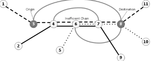
Figure 2: A typical inefficient chain and flow re-routing
We illustrate the idea of re-routing flows by an example shown in Figure 2. The example shows three commodities each with a different line pattern, and a graph where origin node 3 and destination node 8 define a part of the inefficient chain. The re-routing of the flows between nodes 3 and 8 causes individual commodity flow disconnections. The flow re-routings take place independently for each different commodity between its origin and destination nodes, i.e., the commodity shown with the solid black line must travel from node 4 to node 7, the dotted one must travel from node 6 to node 8, and the dashed one from node 3 to node 8. The grey lines depict possible alternative re-routing paths within the network. All three flow re-routings, for this particular example, result in one single neighbour.
Another important component of our ILS is a frequency-based memory fea-ture adopted by Paraskevopoulos et al. (2012) that penalizes potential moves that alter flows that have been changed frequently in previous iterations of
the search. A vector ⃗g of size |A| is used to store each valuegij, which is the
number of times that the value of xpij is changed for some p ∈ P. After an
improvement in the current solution is observed, ⃗g is reinitialized to the zero
vector.
trial solution s′ as
∆fmove(s, s′) =f(s′)−f(s) +β
∑
(i,j)∈A
bijgij, (7)
where β is a scaling parameter, and bij has a value equal to 1 if the arc (i, j)
participates in the current local move from s to s′, and a value 0 otherwise.
The component β∑(i,j)∈Abijgij is added to the cost of the local move to
penalize moves that involve frequently selected arcs.
Trial solutions with smaller values of ∆fmove are generally preferred.
How-ever, it may be that this number is large enough to prevent the search from
selecting a high-quality neighbour s′. To avert such cases, an aspiration
cri-terion is used: if f(s′) < f(sILSbest), the penalty component is ignored so
that ∆fmove =f(s′)−f(s). The neighbourhood search procedure is shown in
Algorithm 3.
Algorithm 3: neighbourhood Search
Input: s′ (current solution),M a large number
Output: s′′ (best neighbour)
min =M;
for All inefficient chains k of s′ and for all combinations of nodes i, j
in k do
PI ← IdentifyDifferentCommodities(k, i, j);
while PI is not empty do if isFeasible(k, i, j,PI) then
s∗ ←CreateNeighbour(k, i, j,PI);
else
RemoveFirstElement(PI);Continue;
if ∆fmove(s, s∗)<min then
s′′←s∗ ; min = ∆fmove(s, s∗) ;
RemoveFirstElement(PI);
In Algorithm 3 the functionIdentifyDifferentCommoditiesforms the listPI
by identifying the different commodities that have positive flows between the
nodesiandj of an inefficient chaink. CreateNeighbourcreates a neighbouring
solution of s′, and RemoveFirstElement removes the first element of the list.
Finally, the isFeasibleis a boolean function that returns “true” if a particular
combination (k, i, j) leads to some re-routing of flow.
3.6.2. Ejection Cycles
A major component of the ILS is its perturbation strategy (Louren¸co,
optimum solution, such that the new diversified solution preserves some infor-mation from the local optimum. The proposed perturbation strategy in this paper, namely Ejection Cycles (EC), applies multiple cycle-based moves in the spirit of ejection chains (Glover 1996). The main idea of the ejection-chains strategy is to apply a compound move consisting of a series of consecutive local moves. Adopting this idea, our EC comprise a series of consecutive cycle moves of the type described in Section 3.6.1. The aim of EC is to perturb the structure of the current solution to achieve diversification, and also to remove some of the inefficient arcs from the solution.
The are two phases to creating the sequence of local moves. The first phase creates inefficient chains to re-route flow using similar ideas to Section 3.6.1, but considers the previous usage of arcs in local moves instead of cost and also allows flows in arcs to violate capacity constraints. The second phase attempts to remove infeasibility by doing further flow re-routing, again using arc usage in determining the path.
We now present more precise details of how our sequence of local moves is determined. In the first phase, we first find a set of inefficient chains and
focus on sub-chains containing at most ζ arcs. For a given sub-chain, the
list PI is formed, and ip, jp and wp are computed. The list of commodities
is scanned and a re-routing of flow is performed for each commodity p of PI
in turn. However, in this re-routing, feasibility with respect to arc capacities is not enforced, as the second phase essentially operates a repair mechanism to restore feasibility. The first phase employs a full re-routing by applying
Dijkstra’s algorithm to find a shortest path fromip tojp, where cost for each
arc (i, j)∈ A is
¯
cij =
{
cijhij +fij(1−y¯ij) if (i, j)∈ F/ ,
∞ otherwise, (8)
where hij −1 is the number of times that arc (i, j) has participated in
a local move, and initialization sets hij = 1 for all (i, j) ∈ A, and F is a
set of forbidden arcs that initially comprises all arcs between ip and jp in
the subchain. The hij values have a similar purpose to the gij values of
Section 3.6.1 except that the method of initialization is different. Also, the
re-initialisation for gij is replaced by a scaling process for thehij. Specifically,
to avoid hij become very large for some arcs (i, j), we periodically divide hij
by hmin for all (i, j) ∈ A, where hmin = min(i,j)∈Ahij. If Dijkstra’s algorithm
returns a shortest path length of infinity, then the current sub-chain is not
considered further and another one is selected. Otherwise, a flow of valuewpis
When re-routing of flow between nodesip and jp of the sub-chain is
com-plete for each p∈ PI, we check if any arc has a flow that violates its capacity
constraint. If there is no violation, then a new feasible solution is found and the EC terminates with a perturbed solution. When some flows violate arc
capacities, we proceed as follows. Let AV denote the set of arcs having a
capacity violation. For all arcs (i, j)∈ AV, a set of commoditiesPI′ is selected
whose removal from (i, j) restores feasibility but keeps the capacity utilisation
of the arc as high as possible. Specifically, the process of repeatedly selecting
a commoditypwith the largest flow xpij in (i, j) is inserted in PI′ and the flow
in (i, j) is reduced byxpij is applied until the flow in (i, j) is reduced to exactly
uij or the next selection would cause the flow in (i, j) to become strictly less
than uij. In the latter case, the final commodity p selected for insertion into
P′
I is chosen to have minimal flow in (i, j) from among those commodities
where the removal of their flow from (i, j) reduces the total flow in (i, j) to
be less than or equal to uij. Having formed PI′, the respective ip, jp and wp
are computed, and infeasibility chains that are formed in the same way as for
inefficient chains, as described in Section 3.6.1.
Having formed the infeasibility chains, the aim is to re-route the flow in the chain using the method described above. More precisely, Dijkstra’s algorithm
to find a shortest path from the the starting node ip of the sub-chain to the
ending node jp, where all arcs between ip and jp of the sub-chain are added
to the set F and costs for the shortest path problem are defined by (8). If
a suitable path for re-routing is found, then the trial solution s∗ is updated.
The process of re-routing flow in other infeasibility chains continues until no capacity violations occur or no further re-routing is possible due to the
constraints imposed by set F. If the former case, the EC terminates with a
perturbed solution. In the latter case, the EC returns to the initial feasible
solution s′, the first commodity of set PI is deleted and EC is applied on
the remaining commodities in the set. As in Section 3.6.1, additional trial
solutions are created by removing the first element of list PI and repeating
the process until PI is empty. The complete procedure is applied to all
sub-chains, and terminates when the first feasible perturbed solution is found. The pseudo code of the EC is given in Algorithm 4.
IdentifyViolatedArcs identifies the set of violated arcs AV. The function
NeighbourExists is a boolean function that returns “true” if there exist an alternative path that the flow can be re-routed, regardless the capacity con-straints at arcs. If no alternative paths are found (in case all neighbouring arcs
have been assigned a cost of infinity), then NeighbourExists returns “false”.
The functionU pdateV iolatedArcsidentifies which of the arcs of the re-routed
paths are violated in terms of capacity constraints and updates the set of
Algorithm 4: Ejection Cycles
Input: s′ (current solution)
Output: s∗ (best neighbour)
for All inefficient chains k of s′ and for all combinations of nodes i, j
do
PI ← IdentifyDifferentCommodities(k, i, j);
while PI ̸=∅ do
***First EC Iteration***
AV ←IdentifyViolatedArcs(k, i, j);
if AV =∅ then
EndAlgorithm;
else
P′
I ← IdentifyExcessCommodities(AV);
***Next EC Iterations*** while PI′ ̸=∅ do
if NeighbourExists(PI′)then
s∗ ←CreateNeighbour′(PI′);
AV ←UpdateViolatedArcs(k, i, j);
if AV =∅then
EndAlgorithm;
else
P′
I ← UpdateExcessCommodities(AV);
else
RemoveFirstElement(PI); PI′ ← ∅;
excess commodities that need to be removed from the violated arcs to restore
capacity feasibility, while similarly U pdateExcessCommodities updates the
excess commodities in the next iterations.
4. Computational Results
Finally, Section 4.6 presents extensive comparison results with state-of-the-art algorithms that have been proposed for the problem.
4.1. Data sets
To evaluate the performance of the proposed algorithm, computational ex-periments are conducted on the C and C+ benchmark instances described in Crainic et al. (2000) and are available online (http://pages.di.unipi.it/frangio/). These sets include instances with 20, 25, 30 and 100 nodes, 10 to 400 com-modities and 100 to 700 arcs, and have been widely used in the literature. These instances differ from one another with respect to the nature of the arc capacities, which are either loose (L) or tight (T), and with respect to the rel-ative importance of fixed costs (F) and the variable flow costs (V) per unit of flow. There also exist benchmark instances described by Alvarez et al. (2005) defined on an undirected graph using edges as opposed to a directed graph using arcs. These define a different problem than the one we address in this paper, as is discussed by Crainic et al. (2000), and is the reason why this set is not considered here.
The proposed algorithm was implemented in a Visual Studio 2010 envi-ronment using the C++ programming language, and all runs were performed on a single core Xeon E5507 2.27 GHz using CPLEX 12.6 as the optimizer.
4.2. Calibration
The proposed Cycle-based Evolutionary Algorithm (CEA) uses five
param-eters; the numberλof initial solutions examined to produce the Reference Set
R, the cardinality µ of R, the cardinality κ of CS, the maximum number δ
of local search iterations without an improvement in the solution quality, and
the maximum numberϑmax of CPLEX calls for which an improvement in the
current solution is not observed. The termination criterion is the computa-tional time. Various time limits were used to test our algorithm according to different time limits used by the state-of-the-art algorithms of the literature.
The scaling parameters α and β are self-calculated during the solution
process, and are equal to the average cost of an arc in the current best solution found, i.e., α=β=f(sbest)/
∑
(i,j)∈Ay sbest
ij . The parameter λ does not appear
to have a significant impact to the quality of the solutions; however, to have an adequate initial population size, we set it to 1500. Another parameter that
seemed not to have significant impact is the size ζ of the sub-chains where
local search takes place (see Section 3.6.1 for details). Parameter ζ was set
We setκ= 3 to preserve the SS character of the proposed algorithm.
Pa-rameter κ needs to be larger than 2 to enhance the recombination process,
but should be relatively small to ensure that a large number of possible com-binations among the solutions of the Reference Set is considered. We tried 4 and 5 which resulted in a poor variety of offspring, due to the limited number of combinations. The latter problem was more prominent in the later SS iter-ations, when convergence is close and the need for different offspring is more apparent.
Parametersδ and ϑmax are interrelated as they typically control the total
number of local search iterations. In particular, ϑ tracks CPLEX iterations;
it is initialized to 1 and is incremented by one unit until ϑmax is reached. At
each iteration, the numberδ of local search iterations is set equal to 10ϑ. Our
experiments indicate that values of ϑmax equal to 6, 7, and 8 are appropriate,
with values below 6 resulting in deterioration in the solution quality, and values greater than 8 slowing down the process without yielding any significant gain in the solution quality.
Table 1 shows the computational experiments conducted to investigate on the algorithm’s behaviour with respect to different sets of parameters. Different parameter sets were used for different groups of problems. For
large-scale problems, the Reference Set was of relatively small sizes and δ was
assigned high values, whereas opposite settings were used for small to medium scale problems, for reasons described above. Table 1 shows the C and C+ benchmark instances classified into 6 groups according to their size. The label for each group is a vector depicting the number of nodes, the number of arcs and the number of commodities. The problem instances within each group differ in the tightness of the arc capacity constraints and the relative importance of the fixed costs and the costs of per unit of flow. The calibration was conducted by using one problem instance from each group, shown in the headings of the six main columns of Table 1. For each instance, ten runs, each with a run time of two hours, were conducted to retrieve the average solution values for each instance shown under the second column for each group. The parameter set that produces the best average (shown in bold font) for each group is fixed and used to solve the rest of the instances in that group to produce the results presented in the tables of this section.
Table 1: Calibration of the algorithm’s parameters
Group 25-100-(10 & 30) 20-(230 & 300)-40 20-(230 & 300)-200
ϑmax, µ 25-100-30FT ϑmax, µ 20,230,40FT ϑmax, µ 20,230,200VT
6,30 86294 6,30 644352 6,30 100343
6,40 86107 6,40 644118 6,40 99457
6,80 85870 6,80 643537 6,80 100317
Parameter 7,30 86333 7,30 644346 7,30 100283
Sets 7,40 86189 7,40 644346 7,40 99560
7,80 85963 7,80 643735 7,80 99607
8,30 86237 8,30 644483 8,30 100023
8,40 86296 8,40 644133 8,40 99939
8,80 85894 8,80 643995 8,80 99786
Best 6,80 85870 6,80 643537 6,40 99457 Group 100-400-(10 & 30) 30-(520 & 720)-100 30-(520 & 720)-400
ϑmax, µ 100-400-30FT ϑmax, µ 30,700,100FL ϑmax, µ 30,700,400FT
6,20 142086 6,20 61045 6,20 134911
6,30 142697 6,30 62209 6,30 134930
6,40 142969 6,40 61872 6,40 135278
Parameter 7,20 142235 7,20 61969 7,20 134745
Sets 7,30 143173 7,30 61414 7,30 135362
7,40 143448 7,40 62182 7,40 135535
8,20 142499 8,20 61658 8,20 134810
8,30 142749 8,30 61648 8,30 134921
8,40 143099 8,40 61937 8,40 135522
Best 6,20 142086 6,20 61045 7,20 134745
Table 2: Indicative t-tests for the results derived by using different parameter settings
Parameter settings (θ1max, µ1), (θ2max, µ2)
25,100,30FT (6,30), (6,80) (7,30), (7,80) (8,30), (8,80) (6,80), (8,80)
p-value 0.011 0.001 0.002 0.171
20,230,40FT (6,30), (6,80) (7,30), (7,80) (8,30), (8,80) (6,80), (7,80)
p-value 0.006 0.047 0.033 0.105
20,230,200VT (6,30), (6,40) (7,40), (7,80) (8,40), (8,80) (6,40), (7,80)
p-value 0.123 0.470 0.459 0.366
100,400,30FT (6,30), (6,20) (7,30), (7,20) (8,30), (8,20) (6,20), (7,20)
p-value 0.196 0.134 0.364 0.433
30,700,100FL (6,30), (6,20) (7,30), (7,20) (8,30), (8,20) (6,20), (8,20)
p-value 0.002 0.045 0.489 0.032
30,700,400FT (6,30), (6,20) (7,30), (7,20) (8,30), (8,20) (7,20), (8,20)
p-value 0.317 0.042 0.402 0.450
by these observations, the size µ of the Reference Set takes larger values for
small to medium scale problems, and relatively small values for the larger scale instances.
We also conducted indicative t-tests for different parameter settings and we include the results in Table 2. Table 2 has six parts that refer to results regarding six different benchmark instances. Each part of the table has two
rows; the first row indicates the pairs of parameters (θmax, µ) and the second
row reports the p-value derived by comparing the two different sets of results derived by 10 runs of the algorithm. As Table 2 shows, for some of the pairs one
[image:22.595.149.451.414.554.2]other the difference is not statistically significant. We select the parameter setting with the best average value (see Table 1), and we keep it fixed for each group of instances to perform our experiments, regardless of the statistical significance status.
4.3. Network efficiency vs total cost
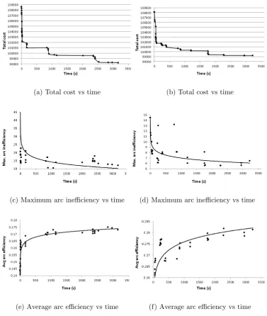
To illustrate the impact of the network efficiency on the solution cost, we have conducted analyses to shed light into the behaviour of the search on two problem instances, namely 20,230,200VT and 30,700,400VL. The network ef-ficiency is defined with respect to either the maximum arc inefficiency or the average arc inefficiency, where the inefficiency measure is as defined in Section 3.6. The results are given in Figure 3, which shows how the two efficiency measures and the total cost change as the search progresses over time, sep-arately for instance 20,230,200VT on the left and for instance 30,700,400VL on the right.
Figures 2(a) and 2(b) respectively show the changes observed in the value of the best solutions found for the 20,230,200VT and 30,700,400VL problem instances over time. Similarly, Figures 2(c) and 2(d) show the maximum inefficiency of an open arc for different solutions found over time. We observe that as the algorithm iterates, the maximum arc inefficiency is dramatically reduced and follows a logarithmic trend. Conversely, Figures 2(e) and 2(f) show an increase in the average efficiency of the arcs as the search progresses, which is indicative of an increase in the overall efficiency of the network as the solution quality is improved.
4.4. The impact of the CEA’s main components on the solution quality
Experimentation was conducted on different versions of the proposed CEA to investigate the effect of various components on the final solution quality.
Three versions of CEA were thus considered: (i) Version “\EC” is where a
random perturbation strategy is used instead of EC. According to this ran-dom strategy, 25% of the commodities are selected at ranran-dom, which are then removed and re-routed via the construction mechanism as discussed in Section
3.4. (ii) Version“\SolvR” replaces the Solvency ratio strategy with a random
strategy for the parent selection and the Reference Set updating criteria. Ac-cording to the random strategy, the parents that comprise the Candidate Set are selected at random and the elitist updating criteria described in 3.5.1 are
used. (iii) Version “\Ineff”, performs local moves on chains composed by all
(a) Total cost vs time (b) Total cost vs time
(c) Maximum arc inefficiency vs time (d) Maximum arc inefficiency vs time
[image:24.595.98.476.165.612.2](e) Average arc efficiency vs time (f) Average arc efficiency vs time
Table 3: Results from different versions of CEA on the benchmark instances of Crainic et al. (2000)
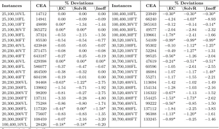
Instances CEA % Deviations Instances CEA % Deviations
\EC \SolvR \Ineff \EC \SolvR \Ineff
25,100,10VL 14712 0.00 0.00 0.00 100,400,10FL 23949 −0.30* −0.30* −0.30* 25,100,10FL 14941 0.00 −0.09 −0.09 100,400,10FT 66240 −4.24 −4.03* −8.93 25,100,10FT 49899 0.00* −1.34 −1.44 100,400,30VT 385163 −0.12 −0.14 −0.14* 25,100,30VT 365272 0.00* 0.00* 0.00 100,400,30FL 49577 −2.04 −2.84 −2.32 25,100,30FL 37324 −0.53 −2.15 −1.56 100,400,30FT 139661 −1.78* −2.41 −1.66 25,100,30FT 85530 −0.54 −0.54 −0.77 30,520,100VL 54109 −0.99* −0.99* −0.99* 20,230,40VL 423848 −0.05 −0.05 −0.07 30,520,100FL 95302 −0.10 −1.12* −1.25* 20,230,40VT 371475 −0.08 0.00 −0.08 30,520,100VT 52284 −0.49 −1.27* −1.31 20,230,40FT 643187 −0.27 −0.25 −0.19 30,520,100FT 98525 −0.56* −1.26 −2.04 20,300,40VL 429398 0.00* 0.00* 0.00* 30,700,100VL 47619 −0.24* −0.51* −0.51* 20,300,40FL 586077 −0.37 −0.47 −0.67 30,700,100FL 60596 −1.05 −2.61 −2.55 20,300,40VT 464509 −0.38 −0.32 0.00 30,700,100VT 46084 −1.07 −1.17 −1.48* 20,300,40FT 604198 −0.19 −0.01 0.00 30,700,100FT 55271 −1.17 −1.55 −2.21 20,230,200VL 94468 −0.63* −1.22* −2.75 30,520,400VL 113694 −1.42 −1.02 −1.49 20,230,200FL 139002 −1.54 −0.71 −1.92 30,520,400FL 154134 −1.28 −1.03 −2.16 20,230,200VT 98209 −0.81 −0.27 −2.75 30,520,400VT 116322 −0.67* −1.13 −1.52 20,230,200FT 137131 −3.33 −0.28 −4.80 30,520,400FT 154425 −1.53* −1.73* −2.62 20,300,200VL 75288 −0.86 −0.80 −1.74 30,700,400VL 99222 −0.56* −0.85 −1.50 20,300,200FL 117320 −0.44* 0.00* −1.58* 30,700,400FL 137112 −1.84 −2.25 −3.83 20,300,200VT 75607 −0.83 −0.83 −1.35 30,700,400VT 96388 −1.13* −1.20* −1.61 20,300,200FT 108459 −0.07 −2.16 −3.20 30,700,400FT 133245 −0.89* −0.25 −1.46 100,400,10VL 28426 −0.18* −0.18* −0.20
*not statistically significant
is limited to two hours. The values under column “% Deviations” in Table 3 show the percent deviations of the solution values obtained by the three versions of the CEA from those of the best solution value. In particular, the
deviations are calculated as 100(v(CEA)−v(Alg))/v(CEA), where v(Alg) is
the solution value obtained by one of the three versions of CEA. We conducted statistical t-tests between the runs of CEA and the runs of different versions of CEA, and an asterisk is put next to the deviation when the tests were not significant.
From Table 3, it can be easily observed that the impact of the EC in the quality of the final solution is significant, and can yield reductions of up to
4.24% in total cost. The maximum improvements afforded by the Solvency
Ratio and the Inefficiency Measures are 4.03% and 8.93%, respectively. A
negative deviation value in this table indicates that the solution found by the CEA is better. On average, the most significant impact comes from the
Inefficiency Measures component with an average deviation of −1.56%. The
same statistics for the Solvency Ratio and the EC are −0.96% and −0.80%,
4.5. Solvency Ratio vs random parent selection
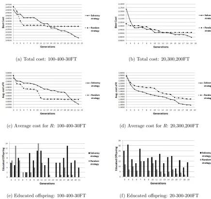
To illustrate the effectiveness of the Solvency Ratio, tests were conducted on two instances, namely 100-400-30-FT and 20,300,200FT, for the reason that these two instances typically present the general behaviour of the algorithm using solvency-based and random parent selection strategies.
Figure 4 presents the comparisons between the two strategies. The first two SS iterations are used as a warm up for the solvency strategy, which is enabled from the third SS iteration onwards as is apparent from the figures. Figures 3(a) and 3(b) show how the best solution values evolve over time. For 100,400,40FT, it is easily seen that solutions obtained by the random-based strategy are quickly trapped in a local optimum, whereas the solvency-based strategy is slower to improve the best solution initially, but displays a gradual yet continual reduction in the overall cost as the generations evolve, and terminates with a better overall solution. Instance 20,300,200FT exhibits a similar pattern, i.e., the solvency strategy provides a large improvement in the early SS iterations and then follows a less steep drop as the algorithm continues to improve the total cost. The random strategy is again trapped in a local optimum at iteration 12. Figures 3(c) and 3(d) show the changes in the average solution cost in the Reference Set over the SS iterations. The main observations on the behaviour of the solvency-bases strategy are similar to the first two figures.
A “healthy” evolutionary process should typically produce a decent num-ber of educated offspring at each SS iteration. Figures 4(e) and 4(f) show that this is also the case in the proposed algorithm. In particular, the figures show that the random strategy has difficulties in producing educated offspring and therefore results in premature convergence. In contrast, the solvency strat-egy is able to update the Reference Set with educated offspring even near termination.
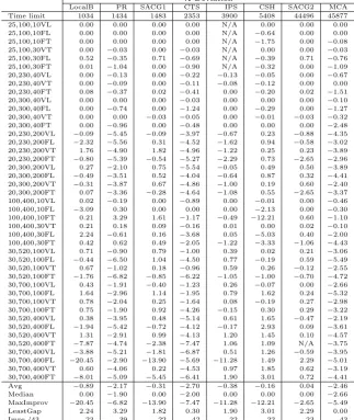
4.6. Comparative analysis
In this section, we report comparative computational results of the pro-posed algorithm with the Cycle-based Tabu Search (CTS) of Ghamlouche et al. (2003), Path Relinking (PR) by Ghamlouche et al. (2004), Multilevel Coop-erative Algorithm (MCA) by Crainic et al. (2006), Capacity Scaling Heuristic (CSH) by Katayama et al. (2009), IP Search (IPS) by Hewitt et al. (2010), the two algorithms based on Simulated Annealing and Column Generation (SACG1 and SACG2) described by Yaghini et al. (2013) the results for which are reported with time limits 600 and a 18000 seconds, respectively, and
Lo-cal Branching (LoLo-calB) by Rodr´ıguez-Mart´ın and Salazar-Gonz´alez (2010).
(a) Total cost: 100-400-30FT (b) Total cost: 20,300,200FT
(c) Average cost forR: 100-400-30FT (d) Average cost forR: 20,300,200FT
[image:27.595.97.534.178.589.2](e) Educated offspring: 100-400-30FT (f) Educated offspring: 20-300-200FT
tested here; instead they use their own benchmark instances. The reason for not being able to test our algorithm on the Alvarez et al. (2005) benchmark set is that these instances are based on an undirected graph and work with edges, whereas the problem we solve is on a directed graph and our algorithm has been developed to operate on arcs.
Table 4 shows the comparison results where the first column shows the name of the instance as characterized by the number of nodes, the number of arcs and the number of commodities. The solution values obtained by the proposed algorithm are reported under column “CEA”. The remaining five columns report the relative percentage deviations of the solution values found by the CEA from those reported by the papers quoted above, and is calculated
as 100(v(CEA)−v(Alg))/v(CEA), where v(Alg) indicates the solution value
produced by the corresponding algorithm andv(CEA) the solution value
pro-duced by the CEA. A negative value indicates that the solution found by the CEA is better.
The first seven rows describe, to the best that we were able to extract,
the computational resources used to run the algorithms. The row titled
“T.Lim.(sec)” reports the time limit used by the authors of the correspond-ing algorithm, whereas the “Used Cores” row indicates how many cores from the original configuration of the CPU were used to run the algorithm. It is assumed that the computational power increases linearly with the number of cores used. Due to different computing facilities, we have normalized the com-putational times using the approach described in Dongarra (2014) and data from http://www.cpubenchmark.net/. All comparisons were made according to the Passmark CPU Score (PCPUS). As we were unable to find PCPUS for Sun systems on http://www.cpubenchmark.net/, we used the Dongarra (2014) list, and selected an Intel equivalent. The final scores are reported in the row titled “PCPU Score”. The running times were normalized by using CEA as the reference point, i.e., Norm.TL(Alg)= PCPUS(Alg)TL(Alg)/PCPUS(CEA).
The table also reports some summary statistics in the last six rows, in-cluding the median and the average of the deviations. The “MaxImpr.” row shows the maximum improvement afforded by the CEA. The lower this value is, the better the performance of the algorithm. The LeastGap row shows the maximum deviation over instances for which CEA did not find a better solution. Finally, the row named “Impr./43” shows the number of instances out of the total 43 tested, where CEA yielded the same or better results over the algorithm it is compared with.
finds optimal solutions for 25,100,30FT and 20,230,40VL which could not be found by any of the heuristics used for comparisons with the exception of the ones described by Yaghini et al. (2013). The maximum deviations of the
CEA are −8.75% compared with CTS, −8.46% compared with PR, −5.49%
compared with MCA,−12.21% compared with CSH,−11.28% compared with
IPS,−17.07% and −1.06% compared with SACG1 and SACG2, respectively,
and −23.81% compared with LocalB.
Noteworthy is the fact that on large-scale problem instances 20,300,200FT, 100,400,30FT and 30,520,100FT, new best solutions were obtained with values 107546, 139535 and 97856, respectively. These instances have up to 100 nodes,
520 arcs and 200 commodities, and the new best solutions deviate by−0.29%,
−1.06% and −0.70% over the previous best known solutions, respectively.
On average measures, CEA outperforms CTS, PR and MCA by achieving
average improvements of −3.49%, −3.13%, and −2.46%, respectively.
Com-pared with the rest, the CEA still remains competitive with average deviations
sitting at−0.38% from CHS, −0.74% from IPS,−1.09% from SACG1, 0.04%
from SACG2 and −2.24% from LocalB. Compared with CHS, the proposed
algorithm produces better results by −0.37% on average. Similarly, SACG2
produces results that are better by 0.04%. We also note that we are unable to consider the result of SACG2 for instance 30,520,400FT as this value is lower than the lower bound 150009 reported by Katayama et al. (2009), and any comparison for this instance would therefore be misleading.
The above comparisons are based on the results derived by using the run-ning time limits imposed by the original authors. Even though our time limit was 20000 sec, the CEA was able to discover the best solution in less than two hours for most problem instances. In fact 34 out of 43 solutions CEA produces are derived within 2 hours, out of which 9 refer to large scale instances (which are in total 16). For very large-scale instances, improvements were observed in later SS iterations which necessitated additional running time. The latter observation is as one would expect with evolutionary algorithms, i.e., a num-ber of SS iterations are needed in order that the initial population of solutions can be evolved such that high quality solutions can be produced.