Assessing the performance of MODIS NDVI and EVI for seasonal crop yield forecasting at the ecodistrict scale

remote sensing

ISSN 2072-4292 www.mdpi.com/journal/remotesensing

Article

Assessing the Performance of MODIS NDVI and EVI for

Seasonal Crop Yield Forecasting at the Ecodistrict Scale

Louis Kouadio1,†,_{*, Nathaniel K. Newlands}1,_{*, Andrew Davidson}2_{, Yinsuo Zhang}2 and Aston Chipanshi3

1_{Science and Technology Branch (S & T), Agriculture and Agri-Food Canada (AAFC),}

Lethbridge Research Centre, 5403 1st Avenue South, P.O. Box 3000, Lethbridge, AB T1J 4B1, Canada

2 _{AgroClimate, Geomatics, and Earth Observations Division (ACGEO), S & T, AAFC,}

960 Carling Avenue, Ottawa, ON K1A 0C6, Canada; E-Mails: Andrew.Davidson@agr.gc.ca (A.D.); Yinsuo.Zhang@agr.gc.ca (Y.Z.)

3 _{ACGEO, S & T, AAFC, 300-2010 12th Avenue, Regina, SK S4P OM3, Canada;}

E-Mail: Aston.Chipanshi@agr.gc.ca

†_{Current Address: International Centre for Applied Climate Sciences, University of Southern}

Queensland, West Street, Toowoomba, QLD 4350, Australia

*Authors to whom correspondence should be addressed; E-Mails: Amani.Kouadio@usq.edu.au (L.K.); Nathaniel.Newlands@agr.gc.ca (N.K.N.); Tel.: +1-403-317-2280 (N.K.N.);

Fax: +1-403-317-2187 (N.K.N.).

External Editors: Clement Atzberger and Prasad S. Thenkabail

Received: 25 August 2014; in revised form: 10 October 2014 / Accepted: 11 October 2014 / Published: 23 October 2014

ICCYF weak performance. Ecodistricts are areas with distinct climate, soil, landscape and ecological aspects, whereas CARs are census-based/statistically-delineated areas. Agroclimate variables combined respectively with MODIS-NDVI and MODIS-EVI indices were used as inputs for the in-season yield forecasting of spring wheat during the 2000–2010 period. Regression models were built based on a procedure of a leave-one-year-out. The results showed that both agroclimate + MODIS-NDVI and agroclimate + MODIS-EVI performed equally well predicting spring wheat yield at the ECD scale. The mean absolute error percentages (MAPE) of the models selected from both the two data sets ranged from 2% to 33% over the study period. The model efficiency index (MEI) varied between−1.1 and 0.99 and−1.8 and 0.99, respectively for the agroclimate + MODIS-NDVI and agroclimate + MODIS-EVI data sets. Moreover, significant improvement in forecasting skill (with decreasing MAPE of 40% and 5 times increasing MEI, on average) was obtained at the finer, ecodistrict spatial scale, compared to the coarser CAR scale. Forecast models need to consider the distribution of extreme values of predictor variables to improve the selection of remote sensing indices. Our findings indicate that statistical-based forecasting error could be significantly reduced by making use of MODIS-EVI and NDVI indices at different times in the crop growing season and within different sub-regions.

Keywords: ecodistrict; yield forecasting; MODIS; ICCYF; spring wheat

1. Introduction

addition to the red and near-infrared bands), the Enhanced Vegetation Index (EVI) helps minimizing soil background and atmosphere influences in reflectance data [4,19–21]. Both MODIS NDVI and EVI are commonly used in crop yield forecasting (e.g., [5,6,22–24]). MODIS-derived VIs are also ideal for crop monitoring over fragmented agricultural landscapes (i.e., size of the field close to the size of the pixel [25]).

Reliable and timely crop yield forecasting is crucial for policy strategies, trade and market opportunities. It is also important for achieving and sustaining global food security [26]. In Canada, grain crop production (i.e., wheat, barley, corn, canola, and soybean) plays a vital role in the economy (for example a total production of around 63.5 million metric tonnes in 2011 and $17 billion of farm cash receipts were recorded [27]). A recent modeling tool, the Integrated Canadian Crop Yield Forecaster, ICCYF, has been developed for generating in-season crop yield forecasts at regional scale [28]. The tool utilizes historical climate, near-real time RS data and crop field survey in generating probabilistic yield forecasts that are sequentially-updated within the growing season as data becomes available. The ICCYF combines robust statistical techniques for generating in-season yield forecasts well before the end of the growing season and for providing a probability distribution of the forecasted yields at a given spatial unit. Typically, the basic spatial unit considered in crop yield forecasting at regional scales relies on administrative statistical boundaries [7,13,28–30], even when introducing the notion of ecoregion (e.g., [31,32]). Crop yield forecasting at this unit relies on the availability of historical data at these scales. The current crop yield forecasts based on the ICCYF are performed at the Census Agricultural Regions (CARs), which are composed of groups of adjacent census divisions and are used by the Census of Agriculture for disseminating agricultural statistics [33]. However, given the climate variability and the future challenges of the impacts of climate change on agriculture, exploring crop yield forecasting at the ecodistrict (ECD) scale deserves special attention. An ECD is defined as a subdivision of one ecoregion characterized by relatively homogeneous biophysical and climatic conditions [34]. The differentiating characteristics depends on the regional landform, local surface form, permafrost distribution, soil development, textural group, vegetation cover/land use classes, range of annual precipitation, and mean temperature. The improvement in the timeliness and accuracy of crop yield forecasting through the incorporation of near real-time data (both agroclimate and remote sensing) and the use of sophisticated statistical methods should improve our capacity to respond effectively to the future challenges. Running such tools at spatial scales based on common environmental characteristics (i.e., ecological spatial division) is therefore of great interest both from an ecosystem point of view and for a better crop yield forecasting (i.e., aggregation/upscaling of predicted yields).

modeling at the ECD level through the ICCYF will give more insights on how the forecast may be achieved for oriented user groups, as well as a better understanding of the forecast skill at finer scales. In addition, one future development activity of the ICCYF [36] aims to use data from moderate resolution satellites (i.e., MODIS) for assessing the crop vegetation status and to derive VIs.

Therefore, the objectives of this study were: (i) to investigate the use of other RS indices (MODIS NDVI and EVI) as alternative predictors for forecasting spring wheat yields within the forecast model framework (ICCYF) at the ECD scale; (ii) to compare the forecast model performance at the ECD and CAR scales (ecological spatial unit versus statistical spatial unit), especially in CARs with poorer ICCYF performance as pointed by Newlandset al. [28]; and (iii) to understand when to use one RS index over another in a given region and to understand the dynamics during the growing season. Although several studies have related RS data and/or agroclimate indices to spring wheat on the Canadian Prairies, no such studies have been conducted to relate those indices to crop yield at the ECD scale. Thus, our study takes advantage of historical yield data at the ECD scale across the agricultural landscape of western Canada. The findings should help in improving the forecast skill of the ICCYF, namely in regions with high forecast uncertainties and/or high historical yield variability.

2. Materials and Methods

2.1. Overview of the Integrated Canadian Crop Yield Forecaster (ICCYF)

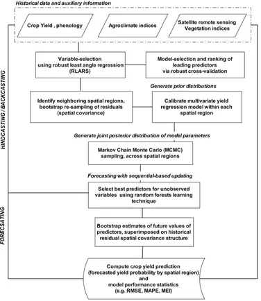
The ICCYF is a modeling tool for crop yield forecasting and risk analysis based on the integration of geospatial and statistical data within a Geographic Information System, developed by Agriculture and Agri-Food Canada (AAFC). The main features [28,36] of the ICCYF are: (1) the integration of a physical based soil moisture model to generate climate based predictors and satellite derived information; (2) an automatic ranking and selection of best predictors using Robust Least Angle Regression Scheme (RLARS) and Leave-One-Out-Cross-Validation (LOOCV) scheme at run time, as well as a spatial correlation analysis among the neighboring spatial units; (3) a Bayesian method for sequential forecasting,i.e., estimation of the prior and posterior distributions of model predictors through a Markov Chain Monte Carlo (MCMC) scheme, and random forest-tree machine learning techniques to select the best predictors of unobserved variables at the time of forecast.

predictors was obtained using the MCMC scheme [41]. For the in-season forecasting, the random forest-tree machine learning technique [42] was used to estimate the required unobserved variables. The estimated variables and the variables observed at near real time were finally used as input into the selected yield model to forecast the yield probability distribution for each ECD. The 10th percentile (worst 10%), the 50th percentile (median) and the 90th percentile (best 10%) were output as the probability measures [28,36]. A detailed description of the modeling methodology can be found in Newlandset al.[28] and Chipanshiet al.[36].

Figure 1.Flowchart describing the crop yield modeling within the Integrated Canadian Crop Yield Forecaster (ICCYF) tool. Adapted from Newlandset al.[28].

The final model at the spatial unit considered is a multivariate regression equation, written as follows:

Yt=γ0+γ1t+ n

X

i=2

where Yi,t is the crop yield for yeart, γ0 is the regression intercept, γ1t refers to the technology trend over time. Xi is the predictor variable, n is the total number of selected predictors, and εt is the error term (independent and normally distributed with mean zero and varianceσ2_{). The technology trend in} yield was assumed to be linear. Extreme values of input data are not taken into account.

2.2. Data

2.2.1. Agroclimate Data

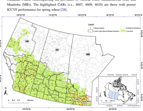
The study region encompassed the three Canadian Prairie Provinces AB, SK and MB (Figure 2), which contains the majority of the agriculture land in Canada. These three provinces account for about 85% of Canada’s arable land [43].

Figure 2. Ecodistricts and Census Agricultural Regions (CARs) across the Western Canadian Prairie (encompassing the provinces of Alberta (AB), Saskatchewan (SK) and Manitoba (MB)). The highlighted CARs (i.e., 4607, 4609, 4610) are those with poorer ICCYF performance for spring wheat [28].

institutions through the Drought Watch activity [46] operated at the National Agroclimate Information Service of Agriculture and Agri-Food Canada (NAIS-AAFC). Also included as agroclimate variable was the growing degree days (GDD) above a base temperature of 5 °C (calculated as the mean daily temperature above a certain threshold base temperature accumulated on a daily basis over a period of time). A detailed description of the calculation of SWA and WDI can be found in Newlandset al.[28]. These agroclimate variables were summed (i.e., GDD) or averaged (i.e., SWA and WDI) for each month from May to August during each growing season. They were then spatially averaged across all stations within a given ECD with equal weighting. For ECDs with no climate data, stations from neighboring ECDs were used.

2.2.2. MODIS-Derived NDVI and EVI Indices

The 16-day MODIS NDVI and EVI composites for Canada south of 60 degree (2000–2010 period) come from the NASA Land Processes Distributed Active Archive Center’s MOD13Q1 products [47]. These products are computed from atmospherically corrected bi-directional surface reflectances that have been masked for water, clouds, heavy aerosols, and cloud shadows [17]. A mask of the Canadian agricultural land [48] was used to process the composites at the ECD level. For our purpose the average value of pixels was kept as the VI value for a given ECD. For all years, the period of MODIS data coverage spanned from the day of year 129 (approximately 9 May) to day of year 273 (approximately 30 September). NDVI is calculated from reflectances in the red and near-infrared (NIR) portions of the spectrum. EVI incorporates reflectance in the blue portion of the spectrum in addition to the red and NIR. The equations are given as follows [19–21]:

N DV I = ρN IR−ρRED

ρN IR+ρRED

(2)

EV I = 2.5 ρN IR−ρRED

ρN IR+ 6ρRED−7.5ρBLU E+ 1

(3)

whereρN IR is the reflectance in the near-infrared portion (841–876 nm),ρRED is the reflectance in the red portion (620–670 nm), andρBLU Erefers to the reflectance in the blue portion (459–759 nm).

Figure 3. Distribution and variability of MODIS NDVI (A) and EVI (B) during the cropping season (May–August) based on historical data, 2000–2010 period. The ends of the boxplots indicate the upper and lower quantiles, the solid line indicates the median. The whiskers are 1.5 times of the box height towards upper and lower from the median. Asterisks are the outliers.

2.2.3. Crop Yield Data

Historical spring wheat yields (all cultivars included) at the ECD scale were provided by Statistics Canada. This yield data for spring wheat was part of a larger historical crop yield federal government database spanning 1992–2010 for Canada’s 38 crops and agricultural area and was intended for AAFC research on crop production and environmental modeling. The estimated yield data were generated from the Field Crop Reporting Series (FCRS). FCRS is a series of six data collection activities using surveys and carried out in order to get accurate and timely estimates of seeding intentions, seeded and harvested area, production, yield and farm stocks of the principal field crops in Canada at the provincial level. Data collected are quality-controlled and compared to previous estimates and other sources when available in order to reduce errors associated to such sample surveys [49]. The official yield estimates of the year is derived from the the November Survey. Only yield data of the 2000–2010 period were included in our study in order to coincide with the MODIS data period (available from 2000 onwards).

2.3. Crop Yield Modeling and Assessment of Model Performance

model candidates, the number of iterations for the model convergence, etc.). Here we tested the EVI in addition to the NDVI. Agroclimate and MODIS-derived VIs were used as predictors of yield forecasting at each ECD level. Therefore, two input data sets were involved: (i) agroclimate plus NDVI indices; and (ii) agroclimate plus EVI indices. The average value of two consecutive 16-day periods of MODIS NDVI/EVI were used. For testing the robustness of the modeling at the ECD scale, the leave-one-year-out cross-validation as performed in Mkhabela et al.[10] and Chipanshiet al. [36] was achieved in this study. For each year of the study period, historical data excluding this year (considered as the forecast year) were used as training data for the yield model at each spatial unit. The forecast was then performed using the data of the forecast year during the growing season (i.e., July, August, and September). The forecasted yield was generated using the observed data from the start of the growing season until the last day of the previous month and the inputs estimated by the tool for the remainder of the growing season.

In order to compare the forecast skills within CARs with poorest ICCYF performance (i.e., CAR 4607, 4609 and 4610, Figure 2), additional runs were performed at the CAR scale over the same period using the input data set as that of [28]. This input data set included historical spring wheat yields, agroclimate variables (i.e., GDD, SWA, WDI), and NOAA-AVHRR NDVI at CAR scale across the Canadian Prairies. CARs with poorest ICCYF performance were previously determined in Newlands et al. [28]. Although RS VIs are already achieved within the ICCYF tool, the use of MODIS-derived VIs aims to investigate their potential for the future development activities. Note that only ECDs with crop land were used in our analysis (207 in this case).

Statistical indicators (i.e., root mean square error-RMSE, mean absolute percentage error-MAPE, and model efficiency index-MEI) were used to quantify the performance of the regression-based models at the ECD scale. The RMSE gives the weighted variations in errors (residual) between the predicted and observed yields. It was calculated as:

RM SE =

v u u t 1 n n X i=1

(Pi−Oi)2 (4)

wherenis the number of observations,Piis the predicted yield andOi is the observed yield. The MAPE is an accuracy measure of the forecast quality and was calculated as:

M AP E = 100 · 1

n n X i=1

Oi−Pi

Oi (5)

The MEI could be considered as a measure of model skill [50]. The closer to 1 the MEI is, the more skillful the model. MEI was calculated as:

M EI = 1 −

" _n X

i=1

(Oi−Pi)2/ n

X

i=1

(Oi−O¯i)2

#

(6)

whereO¯i is the mean observed yield.

Table 1. Top five predictors for all ecodistricts regression models based on input data sets including agroclimate variables combined respectively with MODIS-NDVI (AgMet + NDVI) and MODIS-EVI indices (AgMet + EVI).

Year AgMet + NDVI AgMet + EVI

2000 GDD_6; NDVI_26-28; P_8 GDD_6; P_6; EVI_26-28; GDD_5; P_6 EVI_24-26; EVI_28-30 2001 GDD_6; NDVI_26-28; P_6; GDD_6; EVI_26-28; P_6;

NDVI_24-26; WDI_7 EVI_24-26; EVI_28-30 2002 GDD_8; P_7 ; P_8 GDD_6; P_6; EVI_26-28;

NDVI_22-24; SWA_5 P_8; EVI_24-26

2003 GDD_6; WDI_7; P_7 ; GDD_6; EVI_26-28; P_6; NDVI_26-28; SWA_7 EVI_24-26; P_7

2004 GDD_6; NDVI_26-28; NDVI_24-26; GDD_6; P_6; EVI_26-28; EVI_24-26;

P_7; WDI_5 P_6; P_7

2005 GDD_6; NDVI_26-28; P_7; GDD_6; P_6; EVI_26-28; EVI_24-26; NDVI_24-26; NDVI_34-36 P_7; P_6

2006 GDD_6; NDVI_26-28; NDVI_22-24 GDD_6; EVI_26-28; P_7

P_7; P_8 EVI_24-26; P_6

2007 GDD_6; NDVI_22-24; NDVI_24-26; GDD_6; EVI_26-28; EVI_24-26; NDVI_26-28; SWA_8 P_7; P_8

2008 GDD_6; NDVI_26-28; P_7 GDD_6; EVI_24-26; EVI_26-28; NDVI_24-26; P_6 P_7; P_8

2009 GDD_6; GDD_7; P_7; GDD_6; P_7; EVI_24-26; NDVI_26-28; NDVI_24-26 EVI_26-28; GDD_7

2010 NDVI_26-28; GDD_6; NDVI_24-26; GDD_6; EVI_26-28; EVI_24-26; P_7; NDVI_28-30 EVI_28-30; P_7

Agroclimate variables include growing degree days (GDD), soil water availability (SWA), precipitation (P), and crop water deficit index (WDI). Numbers following these indices,i.e., 5, 6, 7, and 8, stand for May, June, July

and August, respectively; The average of two consecutive 16-day periods of MODIS NDVI/EVI were considered. The number after NDVI/EVI refer to the periods used for the calculation within the year.

3. Results and Discussion

3.1. Selected Predictors at the Ecodistrict Scale

Canadian Prairies was July [53]. Other predominant predictors included agroclimate indices GDD_6 (total GDD of June) and P_6 and P_7 (sums of precipitation in June and July, respectively). In addition, the number of precipitation and temperature related predictors, namely in June and July, reveals that these meteorological factors are important for the final yield of spring wheat.

3.2. Overall Comparison of Yield Model Performance at the Ecodistrict Scale

The comparisons of model performance indicators showed that the results were quite similar when using a data set including either agroclimate and NDVI indices or agroclimate and EVI indices (Figure 4). Overall for models based on agroclimate plus MODIS-NDVI indices, RMSE values ranged from 43 to 957 kg·ha−1 _{over the 2000–2010 period. The ranges of the MEI and MAPE} were −1.1 to 0.99, and 2% to 33%, respectively, for the same period. Satisfactory results were obtained with the coefficient of determination of yield models (median values equaled 0.63). The same ranges of performance indicators were obtained in case of models based on agroclimate indices plus MODIS-EVI indices, with differences occurring in the low values of MEI (i.e., MEI = −1.8) and high values of RMSE (i.e., RMSE = 975 kg·ha−1_{). High ranges of performance indicators suggest that} the models did not capture well the extreme input values. Modeling crop yields by taking into account these extreme values could help improving the model forecast skill. Furthermore, it is worth to note that the MODIS VI is representative of all crops in the area and will be highly influenced by the dominant crops. The consideration of crop specific mask to derive VIs will probably result in improved crop yield forecast models.

Figure 5. 2010 yield forecast of spring wheat- Spatial distribution of model error (CV %) for all ecodistricts and Census Agricultural Regions in yield forecasting using agroclimate and remote sensing indices. (A) agroclimate indices (GDD, P, SWA, WDI) and MODIS-NDVI; (B) same agroclimate indices as previously plus MODIS-EVI; (C) WDI, GDD, SWA and AVHRR-NDVI. MODIS NDVI/EVI values are the average of two consecutive 16-day periods, while AVHRR-NDVI indices are 3-week moving averages.n.a.: not applicable. Note: year was included as an additional input variable in all cases. The mapping of the model performance was based on the crop land extent map.

0 125 250 500Km

±

CV (%)

n.a. 0 - 5 5 - 10

10 - 15 15 - 20 20 - 25 25 - 30

(A) (B)

(C)

2010

3.3. In-Season Crop Yield Forecasting Based on the Two Input Data Sets

The yield forecasts of spring wheat were performed for the months of July, August and September for the 11-year period of the study. Generally, high correlations were obtained for each month of forecast for both input data set used for the modeling: R values greater or equal 0.60, except in 2002 (Tables2and3). Regarding the models based on agroclimate plus MODIS-NDVI indices (Table2), RMSE values ranged from 388 to 940 kg·ha−1, 402 to 911 kg·ha−1, and 403 to 958 kg·ha−1 for July, August, and September forecasts. In case of models based on on agroclimate plus MODIS-NDVI indices (Table 3), the ranges of RMSE values were 361 to 925 kg·ha−1_{, 390 to 906 kg·ha}−1_{, and 395 to 952 kg·ha}−1 _{for July, August,} and September forecasts. Relatively good ICCYF performance was obtained in July, compared with August and September forecasts. This trend was also observed when performing the forecast of spring wheat yield at CAR scale [36]. Ordinarily the forecasted yield gets closer to the actual yield towards the end of the growing season (as more data become available) for a given spatial unit of modeling. However, through the current ICCYF selection algorithm, a yield model may only contain predictors at a few critical stages (e.g., predictors based on observations before July). Thus, predictors based on observations of following months, when becoming available, will have no effect on the forecasted yield. The forecast error and reliability range remain the same for those spatial units. For instance, a great number of models based on July-related predictors and having worst performance will lessen the overall performance of the tool across the study agricultural region. Future research will include assessing how the lead time (time window for which potential predictors, namely RS data, are available before a forecast needs to be/is made) affects the forecast accuracy.

Table 2. Comparison between observed and predicted yields of spring wheat at the ecodistrict scale in Western Canada during the 2000–2010 period. Yield models are obtained using the ICCYF tool (input data set including agroclimate and MODIS-NDVI variables). The forecasts are made for July, August and September. The results are pooled across all ecodistricts.

Year 2000 2001 2002 2003 2004 2005 2006 2007 2008 2009 2010

July

Ra 0.71 0.69 0.34 0.75 0.61 0.60 0.80 0.80 0.83 0.74 0.71 MBEb −578 186 710 77 −133 −170 −57 125 −199 41 47 RMSEc 751 596 940 471 507 553 388 393 404 411 453

August

R 0.70 0.69 0.35 0.75 0.60 0.60 0.76 0.79 0.81 0.74 0.69 MBE −565 173 679 64 −110 −183 −48 115 −194 95 82

RMSE 750 597 911 466 511 560 446 402 417 446 481

September

R 0.71 0.66 0.31 0.75 0.58 0.61 0.76 0.79 0.80 0.73 0.70 MBE −569 152 737 51 −106 −186 −58 122 −206 105 89 RMSE 754 611 958 467 521 555 452 403 430 447 470

a _{Coefficient of correlation;}b_{Mean bias error (kg·ha}−1_{); MBE is the average difference between the predicted}

The comparison of July, August and September forecasts for all ecodistricts on the study region showed noticeable biases (expressed through the mean bias error, MBE) between the observed and predicted yields in 2000 (yield underestimation) and 2002 (yield overestimation) for models based on both two data sets (Tables 2 and 3). In 2002, many North American regions, including the Canadian Prairies, experienced severe drought conditions [35]. Based on our historical input data set, the ICCYF tool failed to capture such extreme conditions. In its current version, extreme value distribution is not taken into account in the forecast models, though the shortness of the study period did not enable more extreme conditions neither. Future works related to the fine tuning of statistical algorithms involved in the ICCYF should help integrating the impacts of extreme conditions.

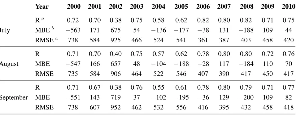
Table 3. Comparison between observed and predicted yields of spring wheat at the ecodistrict scale in Western Canada during the 2000–2010 period. Yield models are obtained using the ICCYF tool (input data set including agroclimate and MODIS-EVI variables). The forecasts are made for July, August and September. The results are pooled across all ecodistricts.

Year 2000 2001 2002 2003 2004 2005 2006 2007 2008 2009 2010

July

Ra 0.72 0.70 0.38 0.75 0.58 0.62 0.82 0.80 0.82 0.71 0.75 MBEb −563 171 675 54 −136 −177 −38 131 −188 109 44 RMSEc 738 584 925 466 524 541 361 387 403 458 420

August

R 0.71 0.70 0.40 0.75 0.57 0.62 0.78 0.80 0.80 0.72 0.76 MBE −547 166 657 48 −104 −188 −28 117 −184 110 70 RMSE 735 584 906 464 522 546 407 390 417 450 417

September

R 0.71 0.67 0.38 0.76 0.55 0.61 0.78 0.80 0.79 0.71 0.77 MBE −551 143 719 37 −102 −195 −36 129 −200 109 82

RMSE 738 607 952 462 532 556 416 395 432 458 418

a_{Coefficient of correlation;}b_{Mean bias error (kg·ha}−1_);c_{Root mean square error (kg·ha}−1_).

3.4. Ecodistrict-Scale Forecast Results in Census Agricultural Region with Poorest ICCYF Performance

CARs, i.e., south-eastern of Saskatchewan, where the trend at ECD scale was the same at CAR scale (CV≤10%, Figure5).

Figure 6. Average values of model efficiency index (A) and mean absolute error percentage (B) of yield models in selected Census Agricultural Regions (CARs) and their corresponding ecodistricts (ECD) during the 2000–2010 period. CARUIDandECDUIDstand for CAR and ECD unit identifiers, respectively. Striped bars represent model performance measures at CAR scale. The selected CARs (i.e., 4607, 4609 and 4610; see Figure2) are those with weak ICCYF performance at CAR scale [28]. The runs at the ECD scale are based on agroclimate (AgMet; i.e., GDD, P, SWA, WDI) and MODIS-NDVI/EVI indices. Whereas those at the CAR scale are based on agroclimate (GDD, SWA, WDI) and AVHRR-NDVI indices.

warmest and most humid in the Canadian Prairies with annual mean precipitation ranging from 450 to 700 mm [54]. A negative relationship has been reported between agricultural productivity and MODIS-NDVI for a maximum threshold of 600 mm in Western Australia [55]. The worst ICCYF performance in the above mentioned ECDS could support this negative relationship between spring wheat yield and MODIS-derived VIs (though the predictors also included agroclimate variables in our case). The weak performance of the ICCYF in CARs across south-eastern Manitoba could be attributed to the soil surface water capacity. Taking into account RS indices that capture the spatio-temporal patterns in surface moisture status (e.g., Normalized Difference Water Index, NDWI [56], or CERES-Photosynthetically Absorbed Radiation [57]) will be explored in future works. Furthermore, exploring the forecast skill of existing approach at ecological scale gives an opportunity for more insights on the impacts of climate variability on crop yield and production.

4. Conclusions

Remote sensing vegetation indices coupled to agroclimate variables are increasingly being used for crop monitoring and crop yield forecasting at regional scales. This study aimed at assessing spring wheat yield forecasting at the ecodistrict scale through an integrated crop yield forecasting approach (i.e., the ICCYF) because of the cohesiveness of the modelling unit in terms of climate and soils. The MODIS NDVI and EVI were respectively coupled to the same agroclimate indices and the performance of the models selected on the basis of these two input data sets was compared across three Western Canadian provinces over a 11-year period (2000–2010). Overall, MODIS NDVI and EVI performed equally well predicting spring wheat yield at the ECD scale. Our analysis also showed that in coarser statistical units (i.e., CAR) with poorer ICCYF performance as reported in previous study, the model performance was improved at that finer and ecological scale. Our findings indicate that statistical-based forecasting error could be significantly reduced by making use of MODIS-EVI and NDVI indices at different times in the crop growing season and within different sub-regions. Downscaling the yield forecasting approach at such specific ecological scale helps in understanding the yield variability within a given statistical unit and improve the forecast skills. Furthermore, exploring the forecast skill of existing approach at ecological scale gives an opportunity for more insights on the impacts of climate variability on crop yield and production.

Acknowledgements

Canada’s 38 crops and agricultural area, and was provided/shared to Agriculture and Agri-Food Canada (AAFC). We thank the anonymous reviewers for their constructive comments.

Author Contributions

Louis Kouadio and Nathaniel K. Newlands are the principal authors of this manuscript having written the majority of the manuscript and performed the analyses. The remote sensing data at the ecodistrict scale across the agricultural landscape of Canada were processed by Andrew Davidson. Aston Chipanshi, Yinsuo Zhang, and Andrew Davidson have reviewed this manuscript and provided comments and suggestions.

Conflicts of Interest

The authors declare no conflict of interest.

References

1. Maas, S.J. Use of remotely-sensed information in agricultural crop growth models. Ecol. Model. 1988,41, 247–268.

2. Boken, V.K.; Shaykewich, C.F. Improving an operational wheat yield model using phenological phase-based Normalized Difference Vegetation Index. Int. J. Remote Sens. 2002, 23, 4155–4168.

3. Reichert, G.; Caissy, D. Reliable Crop Condition Assessment Program (CCAP) incorporating NOAA AVHRR data, a geographical information system, and the Internet. In Proceedings of the Environmental Systems Research Institute (ESRI) User Conference, San Diego, CA, USA, 8–12 July 2002.

4. Hatfield, J.L.; Prueger, J.H. Value of using different vegetative indices to quantify agricultural crop characteristics at different growth stages under varying management practices. Remote Sens. 2010,2, 562–578.

5. Atzberger, C. Advances in remote sensing of agriculture: Context description, existing operational monitoring systems and major information needs. Remote Sens. 2013,5, 949–981.

6. Basso, B.; Cammarano, D.; Carfagna, E. Review of crop yield forecasting methods and early warning systems. In Proceedings of the First Meeting of the Scientific Advisory Committee of the Global Strategy to Improve Agricultural and Rural Statistics, FAO Headquarters, Rome, Italy, 18–19 July 2013.

7. Doraiswamy, P.C.; Hatfield, J.L.; Jackson, T.J.; Akhmedov, B.; Prueger, J.; Stern, A. Crop condition and yield simulations using Landsat and MODIS. Remote Sens. Environ. 2004, 92, 548–559.

8. Becker-Reshef, I.; Vermote, E.; Lindeman, M.; Justice, C. A generalized regression-based model for forecasting winter wheat yields in Kansas and Ukraine using MODIS data. Remote Sens. Environ. 2010,114, 1312–1323.

10. Mkhabela, M.S.; Bullock, P.; Raj, S.; Wang, S.; Yang, Y. Crop yield forecasting on the Canadian Prairies using MODIS NDVI data. Agric. Forest Meteorol.2011,151, 385–393.

11. Kouadio, L.; Duveiller, G.; Djaby, B.; El Jarroudi, M.; Defourny, P.; Tychon, B. Estimating regional wheat yield from the shape of decreasing curves of green area index temporal profiles retrieved from MODIS data. Int. J. Appl. Earth Obs. Geoinf.2012,18, 111–118.

12. Vintrou, E.; Desbrosse, A.; Bégué, A.; Traoré, S.; Baron, C.; Seen, D.L. Crop area mapping in West Africa using landscape stratification of MODIS time series and comparison with existing global land products. Int. J. Appl. Earth Obs. Geoinf.2012,14, 83–93.

13. Johnson, D.M. An assessment of pre- and within-season remotely sensed variables for forecasting corn and soybean yields in the United States. Remote Sens. Environ. 2014,141, 116–128. 14. Mosleh, M.; Hassan, Q. Development of a remote sensing-based “Boro” rice mapping system.

Remote Sens.2014,6, 1938–1953.

15. Whitcraft, A.K.; Becker-Reshef, I.; Justice, C.O. Agricultural growing season calendars derived from MODIS surface reflectance. Int. J. Dig. Earth2014. doi: 10.1080/17538947.2014.894147. 16. Benedetti, R.; Rossini, P. On the use of NDVI profiles as a tool for agricultural statistics: The case study of wheat yield estimate and forecast in Emilia Romagna. Remote Sens. Environ. 1993,45, 311–326.

17. Huete, A.; Didan, K.; Miura, T.; Rodriguez, E.P.; Gao, X.; Ferreira, L.G. Overview of the radiometric and biophysical performance of the MODIS vegetation indices. Remote Sens. Environ. 2002,83, 195–213.

18. Fensholt, R.; Sandholt, I. Evaluation of MODIS and NOAA AVHRR vegetation indices with in situ measurements in a semi-arid environment. Int. J. Remote Sens.2005,26, 2561–2594. 19. Huete, A.; Justice, C.; Liu, H. Development of vegetation and soil indices for MODIS-EOS.

Remote Sens. Environ. 1994,49, 224–234.

20. Jiang, Z.; Huete, A.R.; Didan, K.; Miura, T. Development of a two-band enhanced vegetation index without a blue band. Remote Sens. Environ. 2008,112, 3833–3845.

21. Rocha, A.V.; Shaver, G.R. Advantages of a two band EVI calculated from solar and photosynthetically active radiation fluxes. Agric. For. Meteorol. 2009,149, 1560–1563.

22. Doraiswamy, P.C.; Sinclair, T.R.; Hollinger, S.; Akhmedov, B.; Stern, A.; Prueger, J. Application of MODIS derived parameters for regional crop yield assessment. Remote Sens. Environ. 2005,97, 192–202.

23. Potgieter, A.; Apan, A.; Dunn, P.; Hammer, G. Estimating crop area using seasonal time series of Enhanced Vegetation Index from MODIS satellite imagery. Aust. J. Agric. Res. 2007, 58, 316–325.

24. Bernardes, T.; Moreira, M.A.; Adami, M.; Giarolla, A.; Rudorff, B.F.T. Monitoring biennial bearing effect on coffee yield using MODIS remote sensing imagery. Remote Sens. 2012, 4, 2492–2509.

26. Kouadio, L.; Newlands, N. Data hungry models in a food hungry world—An interdisciplinary challenge bridged by statistics. InStatistics in Action: A Canadian Outlook; Lawless, J.F., Ed.; CRC Press (Taylor & Francis Group): New York, NY, USA, 2014; pp. 371–385.

27. Estimated Areas, Yield, Production and Average Farm Price of Principal Field Crops, in Metric Units, Annual. Avaliable online: http://www.statcan.gc.ca/pub/22-007-x/2012004/ related-connexes-eng.htm (accessed on 19 June 2013).

28. Newlands, N.K.; Zamar, D.S.; Kouadio, L.A.; Zhang, Y.; Chipanshi, A.; Potgieter, A.; Toure, S.; Hill, H.S. An integrated, probabilistic model for improved seasonal forecasting of agricultural crop yield under environmental uncertainty. Front. Environ. Sci. 2014, 2, doi:10.3389/ fenvs.2014.00017.

29. Supit, I. Predicting national wheat yields using a crop simulation and trend models. Agric. For. Meteorol. 1997,88, 199–214.

30. Wu, B.; Meng, J.; Li, Q.; Yan, N.; Du, X.; Zhang, M. Remote sensing-based global crop monitoring: Experiences with China’s CropWatch system. Int. J. Dig. Earth2014,7, 113–137. 31. Mkhabela, M.S.; Mkhabela, M.S.; Mashinini, N.N. Early maize yield forecasting in the

four agro-ecological regions of Swaziland using NDVI data derived from NOAA’s-AVHRR. Agric. For. Meteorol. 2005,129, 1–9.

32. Bolton, D.K.; Friedl, M.A. Forecasting crop yield using remotely sensed vegetation indices and crop phenology metrics. Agric. For. Meteorol. 2013,173, 74–84.

33. Census Agricultural Regions Boundary Files for the 2006 Census of Agriculture-Reference Guide. Available online: http://www5.statcan.gc.ca/olc-cel/ olc.action?objId=92-174-G&objType=2&lang=en&limit=0 (accessed on 16 May 2007).

34. A National Ecological Framework for Canada. Report and National Map at 1:7,500,000 Scale. Avaliable online: http://sis.agr.gc.ca/cansis/publications/ecostrat/index.html(accessed on 31 May 2013).

35. Chipanshi, A.C.; Warren, R.T.; L’Heureux, J.; Waldner, D.; McLean, H.; Qi, D. Use of the National Drought Model (NDM) in monitoring selected agroclimatic risks across the agricultural landscape of Canada. Atmos.–Ocean2013,51, 471–488.

36. Chipanshi, A.; Zhang, Y.; Kouadio, L.; Newlands, N.; Davidson, A.; Hill, H.; Warren, R.; Qian, B.; Daneshfar, B.; Bedard, F.; et al. Evaluation of the Integrated Canadian Crop Yield Forecaster (ICCYF) model for in-season prediction of crop yield across the Canadian agricultural landscape. Agric. For. Meteorol. 2014, under review.

37. Efron, B.; Hastie, T.; Johnstone, I.; Tibshirani, R. Least angle regression. Ann. Stat. 2004, 32, 407–499.

38. Khan, J.A.; Van Aelst, S.; Zamar, R.H. Robust linear model selection based on least angle regression. J. Am. Statist. Assoc.2007,102, 1289–1299.

39. Khan, J., A.S.V.; Zamar, R. Fast robust estimation of prediction error based on resampling. Comput. Stat. Data An.2010,54, 3121–3130.

41. Dowd, M. A sequential Monte Carlo approach for marine ecological prediction. Environmetrics 2006,17, 435–455.

42. Liaw, A.; Wiener, M. Classification and regression by randomForest. R. News2002,2, 18–22. 43. Campbell, C.; Zentner, R.; Gameda, S.; Blomert, B.; Wall, D. Production of annual crops on the

Canadian prairies: Trends during 1976–1998. Can. J. Soil Sci. 2002,82, 45–57.

44. Baier, W.; Robertson, G.W. Soil moisture modelling—Conception and evolution of the VSMB. Can. J. Soil Sci. 1996,76, 251–261.

45. Canadian Soil Information Service. Available online: http://sis.agr.gc.ca/cansis/nsdb/index.html (accessed on 11 July 2014).

46. Drought Watch, Agriculture and Agri-Food Canada. Available online: http://www.agr.gc.ca/ pfra/drought/index_e.htm (accessed on 11 July 2014).

47. NASA Land Processes Distributed Active Archive Center. Available online: https://lpdaac.usgs.gov (accessed on 15 August 2014).

48. Land Cover for Agricultural Regions of Canada, Circa 2000. Available online: http://data.gc.ca/data/en/dataset/16d2f828-96bb-468d-9b7d-1307c81e17b8 (accessed on 11 July 2014).

49. Definitions, Data Sources and Methods of Field Crop Reporting Series. Available online: http://www23.statcan.gc.ca/imdb/p2SV.pl?Function=getSurvey&SDDS=3401 (accessed on 3 October 2014).

50. Murphy, A.H. What is a good forecast? An essay on the nature of goodness in weather forecasting. Weather Forecast. 1993,8, 281–293.

51. A Language and Environment for Statistical Computing. Available online: http://cran.case.edu/web/packages/dplR/vignettes/timeseries-dplR.pdf (accessed on 25 April 2014).

52. Arcgis Desktop: Release 10. Available online: http://www.esri.com/software/arcgis/ arcgis-for-desktop (accessed on 20 October 2013).

53. Basnyat, P.; McConkey, B.; Lafond, G.P.; Moulin, A.; Pelcat, Y. Optimal time for remote sensing to relate to crop grain yield on the Canadian prairies. Can. J. Plant Sci. 2004,84, 97–103. 54. Shorthouse, J.D. Ecoregions of Canada’s prairie grasslands. In Arthropods of Canadian

Grasslands: Ecology and Interactions in Grassland Habitats; Shorthouse, J.D., Floate, K.D., Eds.; Biological Survey of Canada: Ottawa, ON, Canada, 2010; pp. 53–81.

55. Hill, M.J.; Donald, G.E. Estimating spatio-temporal patterns of agricultural productivity in fragmented landscapes using AVHRR NDVI time series. Remote Sens. Environ. 2003, 84, 367–384.

57. NASA Clouds and the Earth’s Radiant Energy System (CERES). Available online: http://ceres.larc.nasa.gov/index.php (accessed on 15 August 2014).