Simulation of irrigation control strategies for cotton using model predictive control within the VARIwise simulation framework

(1)

1

Simulation of irrigation control strategies for cotton using Model Predictive 1

Control within the VARIwise simulation framework 2

3

Alison C McCarthy1*, Nigel H Hancock2 and Steven R Raine3 4

5

* corresponding author 6

7

National Centre of Engineering in Agriculture 8

Institute of Agriculture and the EnvironmentUniversity of Southern Queensland 9

West Street 10

Toowoomba, Queensland 4350 11

Australia 12

13 1

Telephone: 61 7 4631 2189 14

Email: [email protected] 15

Facsimile: 61 7 4631 1870 16

17 2

Telephone: 61 7 4631 2552 18

Facsimile: 61 7 4631 1870 20

21 3

Telephone: 61 7 4631 1691 22

Facsimile: 617 4631 2526 24

(2)

2 Abstract

26

Model-based irrigation control strategies applied to irrigation make decisions (on 27

water application and/or timing) using a crop and/or soil production model. Decisions 28

are made with respect to an optimisation objective which, for irrigation, can be either 29

short-term (e.g. achieving/maintaining a set soil-water deficit) or predicted end-of-30

season (e.g. maximising final yield) by predicting how the crop will respond at the 31

end of the season. In contrast, sensor-based irrigation strategies rely on achieving a 32

performance that is measurable during the crop season to provide the feedback 33

control, and may not necessarily optimise overall crop performance. Model-based 34

control potentially avoids this limitation. 35

36

This paper describes the application of Model Predictive Control (MPC) methodology 37

to the feedback control of irrigation via a model-based irrigation strategy implemented 38

in the irrigation control simulation framework ‘VARIwise’. The requirement to also 39

accommodate spatial and temporal differences in crop water requirement across a 40

heterogeneous field is met by defining management ‘zones’ according to differing soil 41

and crop properties across the field and separately applying the control algorithm for 42

each of these zones. 43

44

Case studies were conducted to evaluate MPC for a centre pivot irrigation machine-45

irrigated cotton crop (under typical Australian growing conditions) with: (i) different 46

in-season performance objectives (maintaining soil-water deficit; maximising square 47

count); (ii) different predicted end-of-season performance objectives (maximising 48

yield; maximising water use efficiency); and (iii) maximising yield with different field 49

(3)

3

significantly higher simulated yields and water use efficiency than an industry-51

standard irrigation management strategy; and (in most but not all situations) direct 52

sensor-based adaptive control strategies. 53

54

Research Highlights 55

• Model Predictive Control was simulated for site-specific irrigation in 'VARIwise' 56

• MPC accommodated both short-term (in-season) and long-term performance 57

objectives 58

• MPC delivered the best performance when optimising crop yield 59

• MPC resulted in higher (simulated) yield than sensor-based strategies 60

• MPC required extensive data to accurately calibrate crop model 61

62

Keywords 63

Variable-rate irrigation, centre pivot, lateral move, scheduling, irrigation automation, 64

Model Predictive Control 65

66

1. INTRODUCTION 67

The development of the control simulation framework ‘VARIwise’ has enabled the 68

evaluation of site-specific, spatially-variable irrigation control strategies on field crops 69

(McCarthy et al. 2010a). VARIwise permits spatially and temporally varied 70

simulation and accommodates sub-field scale variations in all input parameters down 71

to metre-scale zone size. Simulations of ‘sensor-based’ strategies showed potential 72

improvements in yield and water use efficiency (McCarthy et al. 2013). These 73

strategies compared the field measurements with a desired response (e.g. soil-water 74

(4)

4 76

1.1 Model Predictive Control (MPC) applied to irrigation 77

In contrast, an alternative ‘advanced process control’ approach to irrigation uses crop 78

production models to aid the irrigation decision making process. These ‘model-79

based’ control strategies use the available field measurements to calibrate the crop 80

model. The model is then repeatedly executed to determine the optimal irrigation 81

volume and timing that will achieve the desired performance objective (e.g. predicted 82

end-of-season yield). 83

84

The methodology of Model Predictive Control (MPC) involves using a model to 85

predict the optimal input signal at the current time considering future events over a 86

finite time period (Kwon and Han 2005). This is referred to as a ‘control horizon 87

length’. Only the first optimal control action is implemented after each time step. 88

MPC is applicable to irrigation since a soil-plant-atmosphere model may be used to 89

evaluate the application of various irrigation volumes on a fixed number of 90

consecutive days; for example, the model may be used to, firstly, determine the best 91

irrigation volume to apply on each zone for each of the next three days; and, secondly, 92

determine which day resulted in the best overall performance. The future process 93

outputs used to evaluate the irrigation scheme may be predicted daily with 94

measurements of crop response (e.g. for cotton, square/boll count, leaf area index) or 95

soil-water. Alternatively, the simulated final crop yield or water use efficiency may 96

be used to evaluate the various irrigation schemes. 97

98

From the control perspective, the ‘process model’ evolves during the growth of the 99

(5)

5

used by the MPC strategy must be continuously re-calibrated using the currently 101

available field data. The plant growth and soil-water dynamics in the cotton model 102

OZCOT (Wells and Hearn 1992) implemented within VARIwise, can be accurately 103

calibrated (McCarthy et al. 2011. The calibrated OZCOT model has also been found 104

to accurately simulate yield (Richards et al. 2001). Using one season’s field 105

experiment data McCarthy et al. (2011) found that OZCOT was most effectively 106

calibrated (and therefore able to predict the soil and crop response to irrigation 107

application) using full data input, whilst for situations where only two data inputs 108

were available, the simulations suggested that either weather-and-plant or soil-and-109

plant inputs were preferable. 110

111

Park et al. (2009) developed two MPC systems for centre pivot irrigation which both 112

used measured soil and weather inputs to calibrate a soil-water model. Their first 113

implementation used the calibrated model to determine the irrigation volumes which 114

would fill the soil profile for irrigation events on fixed days; whereas their second 115

implementation used the calibrated model to determine the irrigation timing for a 116

fixed irrigation volume application which would fill the soil profile. Neither 117

implementation incorporated the crop growth response. 118

119

1.2 MPC and crop production models 120

The performance objectives set for MPC applied to irrigation can range from a short-121

term objective such as achieving a preset soil-water deficit following each irrigation 122

to a ‘whole season’ objective such as maximising predicted end-of-season yield. 123

(6)

6

In addition, crop production models (such as OZCOT for cotton, discussed below) 125

have sophisticated prediction capabilities which may be utilised in the implementation 126

of MPC. For example, a performance objective to maximise the number of plant 127

fruiting sites during growth should maximise potential predicted end-of-season yield. 128

This additional crop response capability typically requires measurements of the plant 129

to calibrate the crop production model according to the measured plant growth 130

parameters (e.g. fruiting), which in turn requires infield plant sensors to provide 131

calibration data. To maximise uptake of the site-specific irrigation control system by 132

growers it is desirable to minimise the sensor requirements. A reduction in 133

measurements could be achieved by using only the data types that are more influential 134

in the model calibration or by reducing the spatial or temporal resolution of data. 135

However, the data used to calibrate the model should still enable sufficient accuracy 136

of the model. An insufficient range of measurements to calibrate the model used by 137

MPC will influence the accuracy of the model and the model’s ability to predict 138

irrigation and crop performance. 139

140

Hence, this paper aims to: 141

• identify the optimal combination of performance objective and data input 142

combination amenable to practical MPC strategies; and also 143

• explore the impact of different control horizon lengths (period of time for 144

forecasting future events) on the performance of MPC. 145

146

The strategies simulated in this paper explore the viability of the use of MPC in the 147

simulation of a ‘realistic’ irrigation situation with spatial and temporal variation 148

(7)

7

the MPC methodology in VARIwise and, for the example of cotton grown in 150

Australia, presents results for a range of simulations having different performance 151

objectives. The results are presented as three case studies, A, B and C, which, in 152

order, evaluate the potential of MPC to optimise: 153

A. short-term responses of square count or soil-water; 154

B. predicted end-of-season crop yield or water use efficiency with (i) low and high 155

soil nitrogen content, and (ii) crop seasons with and without rainfall; and 156

C. predicted end-of-season crop yield with different combinations of sensory input 157

data to calibrate the model. 158

A comparison is then made between the MPC strategies and simulations of ‘sensor-159

based’ strategies for adaptive irrigation control (McCarthy et al. 2013). 160

161

2. IMPLEMENTATION 162

The simulation framework ‘VARIwise’ (McCarthy et al. 2010a) was created to 163

develop, simulate and evaluate site-specific irrigation control strategies for centre 164

pivot and lateral move irrigation machines on non-uniform (spatially and temporally 165

varied) fields. The framework enables evaluation of strategies with different sensor 166

data availability (both spatial and temporal); for example, the performance of the 167

control strategies with spatial gaps in measured response is explored in McCarthy et 168

al. (2010b). In addition, the framework can provide evaluation of different irrigation 169

system capacity constraints and when supplied with real-time weather and/or other 170

field data, the framework will provide direct machine actuation. 171

172

For the simulation (and management) of cotton irrigation, the cotton production 173

(8)

8

automatically and continuously calibrated according to the currently available 175

weather, soil and plant data. Details are set out in McCarthy et al. (2011). To 176

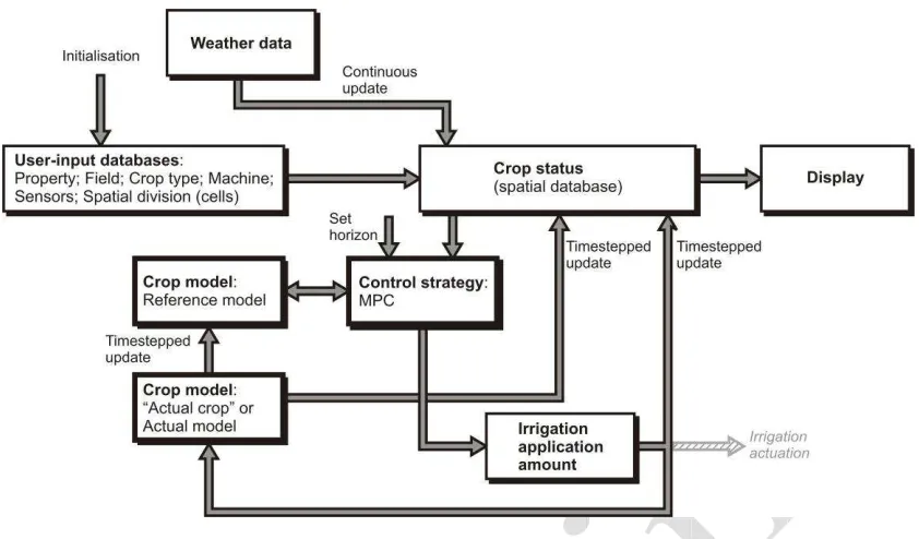
illustrate the VARIwise configuration used to evaluate MPC a general schematic is 177

presented in Figure 1, in which the central blocks and data flows are explained in the 178

following sections. 179

180

Insert Figure 1 here 181

182

The MPC algorithm predicts how much each output (e.g. soil-water, fruit load) will 183

deviate from a time series trajectory within the prediction horizon. A MPC cost 184

function J(k) is calculated for each possible set of input actions in the current time 185

step k using a least squares algorithm of the following form (Maciejowski 2002): 186

187

(1) 188

189

where: 190

J(k) = cost function at instant k

C = length of prediction/control horizon N = number of system outputs

= weighting coefficient for output j

= predicted value of jth output at future instant

= target value of jth output at future instant

191

The control action that minimises the cost function (i.e. that produces the smallest 192

(9)

9

optimisation is repeated at each sample time step to update the optimal input 194

trajectory after a feedback update. Hence, this MPC algorithm calculates the 195

sequence of control action adjustments over a specified future time interval. 196

197

In an irrigation context, the system outputs used to calculate the cost function will 198

typically have different units and magnitudes, and the same percentage change in 199

variables of different units and magnitudes may cause unintentional bias toward 200

variables that are generally larger in magnitude. For example, a particular percentage 201

difference in soil-water will produce a larger cost function than the same percentage 202

difference in leaf area index. Hence, the MPC algorithm was modified (equation 2) to 203

calculate a performance index that represents a percentage difference in the predicted 204

outputs rather than a least squares objective function (equation 1). The control action 205

that maximises the performance index PI(k) is then implemented in each time step, 206

and is calculated using the equation: 207

208

(2) 209

210

The MPC methodology was implemented to determine irrigation timing and site-211

specific irrigation volumes on a daily basis by means of the following four-step 212

procedure: 213

1. Update measured and forecast weather data 214

2. Calibrate crop model 215

3. Optimise irrigation volume for each zone 216

4. Optimise day of next irrigation 217

(10)

10

The details of each step in relation to the following case studies are set out below. 219

This procedure is independently applied to each ‘management zone’, where each zone 220

in the field is defined according to differing soil and crop properties across the 221

heterogeneous field. 222

223

2.1 Step 1: updating measured and forecast weather data 224

For each day of the crop season, the meteorological data input file for the integrated 225

crop model was updated to include the previous day’s weather and the updated 226

weather forecast for the farm’s location. In a field implementation of MPC, the 227

‘previous day’s weather’ could be obtained from an on-site weather station and the 228

‘updated weather forecast’ could be obtained from the Bureau of Meteorology. 229

However, to simulate the performance of MPC for a whole season (where there was 230

no field implementation) both ‘previous day’s weather’ and ‘updated weather 231

forecast’ had to be obtained from historical data. 232

233

Because of the high variability of Australian climate and the difficulty in picking a 234

‘typical’ year, an artificial daily meteorological dataset was created by averaging the 235

day-on-day data of the five years (1999 to 2004 inclusive) appropriate to the location 236

of Dalby (Latitude -28.18°N E, Longitude 151.26°), a major cotton-growing region of 237

south-east Queensland, Australia, and this dataset was used for all simulations. Daily 238

data comprised maximum and minimum temperature, solar radiation and rainfall, and 239

was sourced from Australian Bureau of Meteorology SILO patched point 240

environmental dataset (QNRM 2009). SILO is an enhanced climate database 241

containing Australian climate data from 1889. 242

(11)

11

Forecast weather data, to be used predictively during the simulations, was created by 244

imposing a Gaussian distribution of variability on the daily values of the five-year-245

averaged dataset using standard deviations of ±5°C, ±5°C, ±5 W.hr/m2 and ±50% for 246

maximum temperature, minimum temperature, daily solar radiation and rainfall, 247

respectively; i.e. for any given day, the forecast one, two and three days ahead, then 248

values for each variable randomly generated within each distribution by taking that 249

day’s values as the mean. For each day, only three days of the forecast weather data 250

were used. This is because the two Australian short-term numerical weather 251

prediction models forecast three and seven days ahead and are combined to improve 252

the prediction accuracy (Ebert 2001). The three-day forecast would be more accurate 253

than one model on its own because both models could predict weather to three days. 254

A three-day forecast would ensure short-term prediction accuracy in the predictions, 255

particularly as regards rainfall in south-east Queensland, Australia, where the summer 256

rainfall is dominated by frontal bands of isolated cumulo-nimbus storms. 257

258

2.2 Step 2: calibrating the crop model – ‘actual’ and ‘reference’ models 259

The crop model OZCOT is utilised by VARIwise and can be automatically and 260

continuously calibrated according to the ‘currently’ available weather, plus soil and 261

plant data, using the procedure set out in McCarthy et al. (2011). The procedure for 262

calibrating the production/growth model OZCOT in a real-time implementation, i.e. 263

for actual irrigation machine control, involves automatically and iteratively adjusting 264

the parameters used to predict soil water status and plant growth until the difference 265

between the predicted and sensed variables reached a minimum. For the cotton model 266

OZCOT, the plant variables (leaf area index, boll count, square count), soil variables 267

(12)

12

minimum and maximum temperature, rainfall and solar radiation in weather input 269

file) are interdependent. The plant behaviour can be calibrated by adjusting 270

parameters in a crop properties file, whilst the soil moisture behaviour was calibrated 271

by adjusting parameters in a soil properties file. These parameters were adjusted 272

between the minimum and maximum values of the corresponding parameters in the 273

predefined soil properties and crop variety parameter profiles. The parameters 274

adjusted in the crop properties file included squaring rate (the rate of new flower buds 275

being produced), growth rate of leaf area and plant population constant; whilst the 276

parameters adjusted in the soil properties file were the initial soil moisture content and 277

drained upper limit in each soil layer. 278

279

A ‘reference’ model, labelled ‘RefModel’, is used to provide the crop growth 280

prediction scenario for MPC. However, for the present case studies there was no 281

measured field data input to calibrate the model. To overcome this, a second OZCOT 282

model of the cotton crop was used in place of ‘actual’ field conditions. This model is 283

referred to as the ‘actual crop’ model, labelled ‘AcModel’ and the parameters were 284

different to those in RefModel to emulate RefModel not exactly following the field 285

conditions. In a field implementation the AcModel is not required as field 286

measurements would be used. AcModel was then used to calibrate RefModel (Figure 287

1). 288

289

The crop and soil properties of AcModel were obtained from the user-specified soil 290

and plant measurements (and these varied between simulations, as set out below). 291

Within RefModel the crop variety was specified by the user at commencement. 292

(13)

13

areal variation in available soil-water imposed via a Gaussian distribution of 294

variability having a standard deviation of ±25 mm (water depth equivalent). 295

296

2.3 Step 3: optimising irrigation volumes for each zone 297

Optimal irrigation volumes were determined by iteratively simulating the daily 298

application of sixteen different irrigation volumes at 1 mm increments between 0 and 299

15 mm on each zone in the field. For each irrigation volume applied (for management 300

zone k), a performance index PI(k) was calculated using equation (2). For variables 301

that are maximised to achieve the optimal irrigation strategy (e.g. square count, yield, 302

crop water use efficiency), the target value is taken to be the maximum realistic 303

commercially attainable value (e.g. 15 bales/ha for cotton yield, 3 bales/ML for crop 304

water use efficiency). 305

306

The predicted process outputs used to calculate the PI were taken one day after the 307

irrigation application. The optimal irrigation volume for each zone was the irrigation 308

volume with the highest PI; however, if more than one irrigation volume had the same 309

PI then a water-efficient approach was taken and the optimal irrigation volume was 310

the lowest quantitative volume that achieved the maximum PI. The irrigation volume 311

was then calculated for each zone in the order in which the irrigation machine was to 312

pass over the field. 313

314

2.4 Step 4: optimising the timing (day) of the next irrigation 315

The optimal day for the next irrigation event was determined using the calibrated 316

RefModel. This involved performing the irrigation volume optimisation of the 317

(14)

14

the assumption that the irrigation event could occur on only one of the days. The 319

maximum horizon length was set to three days since three days of predictive weather 320

were used. 321

322

The sixteen irrigation volumes tested on each zone depend on the irrigation day being 323

tested. This is because, unless rainfall occurs, it was assumed that the crop water 324

requirement (and hence irrigation application volume) increases for each day the 325

irrigation event is delayed. For the first day irrigation volumes of 0 to 15 mm were 326

tested with increments of 1 mm; for the second day 0 to 31 mm were tested with 327

increments of 2 mm; and for the third day 0 to 47 mm were tested with increments of 328

3 mm. 329

330

A PI is calculated for each irrigation day by summing the individual PI values for 331

each zone. The day with the highest total PI is taken to be the optimal day for the 332

next irrigation event. The irrigation event is scheduled if the first day in the horizon 333

had the highest PI and there are a minimum number of zones requiring irrigation 334

greater than 0 mm. This ensures that the irrigation application is practical and 335

irrigations are not initiated for only a small number of zones in the field. The 336

threshold, i.e. the minimum proportion of zones requiring irrigation, was arbitrarily 337

selected to be 15% for the case studies presented. 338

339

2.5 Subsequent iteration 340

After the optimal irrigation action – which may, of course, be a ‘nil irrigation’ action 341

(15)

15

subsections above was repeated every day throughout the crop season, with the 343

irrigation events ending on a day specified by the user. 344

345

3. MPC CASE STUDY A: optimisation of short-term responses using different 346

combinations of daily input data 347

The MPC strategy was evaluated with daily input data to predict and control irrigation 348

applications to achieve either a short-term soil (e.g. deficit) or plant growth (e.g. leaf 349

area index) target. A range of combinations of input variables for control were used 350

to determine which input data stream was most useful for MPC. 351

352

3.1 Methodology for Case Study A 353

The field was automatically divided into 44 zones, each of area approximately 0.3 ha, 354

and the irrigations occurred daily. This number of zones enabled the simulations to be 355

executed in a timely manner with spatially variable soil properties across the field. 356

The MPC strategy was evaluated for ten combinations of data input (Table 1). The 357

input data combinations represent the data used both as input variables to calibrate 358

RefModel and the variables used for control. For the simulations using both soil and 359

plant data, the weighting on each variable was set to be 0.5. The strategies with soil 360

data input aimed for soil-water deficit equal to 10% of the plant available water 361

capacity in each zone. 362

363

Insert Table 1 here 364

365

In each simulation, the RefModel (to be calibrated) used the Siokra V16RR cotton 366

(16)

16

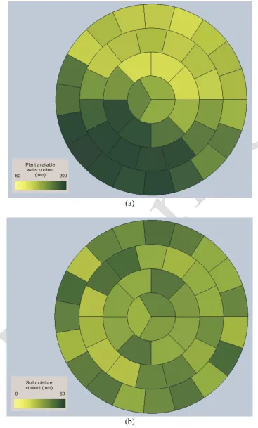
starting soil-water deficit as set out in Figure 2. The starting soil-water deficit map 368

was generated by assigning a starting soil-water deficit value of 30 mm across the 369

field and imposing a Gaussian distribution of variability with standard deviation ±10 370

mm on each zone. The PAWC map was generating by assigning PAWC values of 60, 371

150 and 200 mm on three zones of the fields, spatially interpolating the PAWC using 372

ordinary kriging and by similarly imposing a Gaussian distribution of variability with 373

standard deviation ±10 mm on each zone. The PAWC ranges from 60 to 200 mm in 374

the simulated field to ensure the control strategies could deal with the different soil 375

types that often exist within fields. 376

377

379

The measured crop response (AcModel) used the Sicot 73 cotton variety and soil 380

variability map of Figure 2. Siokra V16RR is a “Roundup Ready” late-maturing 381

cotton variety, whilst Sicot 73 is a full season cotton variety with high yield potential 382

(CSD 2009). The prediction horizon was one day and it was practical for irrigation 383

events to occur daily. 384

385

3.2 Case Study A – Results and discussion 386

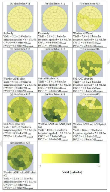
Table 2 sets out the numerical results of the MPC Case Study A, whilst Figure 3 387

illustrates the spatial variability of the yield for each simulation of the case study. The 388

performance of the control strategies are compared based on the average and 389

variability of the yield, irrigation applied, Irrigation Water Use Index (IWUI) and 390

Crop Water Use Index (CWUI) across the zones in the field. The variability reflects 391

(17)

17

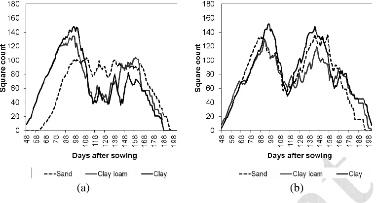
The strategies that use weather-and-plant data to calibrate and target a fixed soil-393

water (simulation #19) and maximise square/boll count (simulation #20), are also 394

compared using the simulated soil-water deficit (Figure 4) and simulated square count 395

(Figure 5) throughout the crop season. 396

397

402

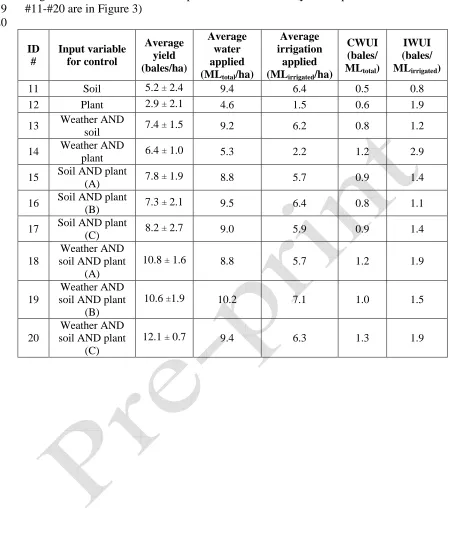
The simulated yield and water use efficiency increased as more data streams were 403

included in the input data combination. This is shown in Table 2 as the single-input 404

simulations produced the lowest yields and water use efficiencies (simulations #11 405

and #12) while the three simulations having three data inputs (simulations #18, #19 406

and #20) performed better than all of the five simulations having two data inputs 407

(simulations #13 to #17 inclusive). 408

409

The data combinations with soil data and no plant data (simulations #11 and #13) 410

resulted in higher yields than those with plant data and no soil data (simulations #12 411

and #14). This result suggests that if only one data input is available then soil data 412

input is most effective for calibrating RefModel and for irrigation control. The 413

simulations using combinations of soil and plant data input to determine the irrigation 414

volumes (simulations #15 and #18) generally produced lower yields and water use 415

efficiencies than those using only plant data input to determine the irrigation volumes 416

(18)

18

example, for the strategies with soil and plant data available to calibrate RefModel, a 418

higher yield was simulated when the strategy maximised the square/boll count 419

(simulation #17) than when the strategy attempted to both maintain soil-water and 420

maximise square count (simulation #15). Hence, in this case there was no obvious 421

benefit in the using multiple variables to determine the application volumes. 422

423

The MPC strategy accurately maintained the soil-water deficit threshold during low 424

rainfall periods of the crop season for simulation #19 (63 to 85 days after sowing, 425

Figure 4(a)). For the MPC strategy that maximised square/boll count (simulation 426

#20), the soil-water deficit was always higher than the soil-water deficit threshold that 427

was approximately maintained in simulation #19 throughout the crop season (Figure 428

4(b)). The soil-water deficit was also lowest in the sand zone (with the lowest plant 429

available water capacity) and highest in the clay zone (with the highest plant available 430

water capacity) throughout the crop season for the strategy optimising square count. 431

This indicates that to maximise the square count, the soil-water deficit should be 432

reduced in proportion with the plant available water capacity of the soil. 433

434

The highest yield was achieved using weather-soil-and-plant input and maximising 435

square count (simulation #20). The square count was higher throughout the crop 436

season for this simulation compared with that for MPC maintaining soil-water deficit 437

(simulation #19) (Figure 5). Hence, the implemented MPC strategy successfully 438

increased the simulated square count and improvements in yield (by 14%) and crop 439

water use efficiency (by 30%) were observed by maximising square count instead of 440

targeting soil-water. 441

(19)

19

4. MPC CASE STUDY B: optimisation using a predicted end-of-season yield or 443

water use efficiency target 444

The MPC strategy uses RefModel to forecast the response of cotton crop with specific 445

environmental conditions and soil and crop properties; hence, the irrigation 446

volume/timing may be adjusted to achieve a desired predicted end-of-season output, 447

in this case a final yield or water use efficiency. This is in contrast to Case Study A in 448

which the MPC strategy used daily input data (e.g. square count, soil-water) to predict 449

the best short-term response to a range of irrigation volumes. 450

451

4.1 Methodology for Case Study B 452

The field was automatically divided into 44 zones as per the previous case study and 453

the irrigations could occur daily. The MPC strategy was evaluated for crop seasons 454

with and without rainfall and with two levels of initial nitrogen content (120 kg/ha 455

and 250 kg/ha). The same weather dataset was used for both these sets of 456

simulations; however the daily rainfall was set to zero for the simulations without 457

rainfall. In the simulations with rainfall there was high rainfall during days 63 to 85 458

after sowing. 459

460

The MPC strategy was used to optimise the predicted Irrigation Water Use Index 461

(IWUI), Crop Water Use Index (CWUI) and yield assuming the machine capacity 462

enabled the machine to traverse the field once every day. An algorithm maximising 463

IWUI or CWUI may decide to apply no irrigation to minimise the irrigation volume 464

but would also produce low yield. Hence, to ensure that the IWUI and CWUI 465

optimisation would irrigate the crop, the minimum acceptable yield was arbitrarily set 466

(20)

20 468

4.2 Case Study B – Results and discussion 469

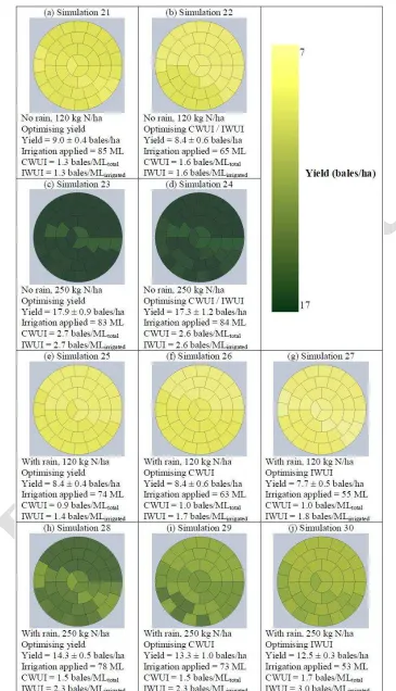
The simulation results are displayed in Table 3 and Figure 6 and the spatially varied 470

irrigation volumes applied are compared with different in-season rainfall and starting 471

nitrogen content at commencement (Figure 7 and Figure 8, respectively). 472

473

478

For each set of field conditions (i.e. starting nitrogen content and in-season rainfall), 479

the simulated yield was highest for the MPC strategy that optimised yield (simulations 480

#21, #23, #25 and #28). Similarly, the strategies optimising IWUI (simulations #27 481

and #30) and CWUI (simulations #26 and #29) produced the highest respective IWUI 482

and CWUI of the simulations with the same field conditions. This indicates that MPC 483

strategy could adjust the irrigation application to improve either yield or water use 484

efficiency. 485

486

Increasing the starting nitrogen content significantly improved the simulated yield and 487

water use efficiency. This is shown in Table 3 as the yield for the no-rainfall 488

simulation with the higher nitrogen content of 250 kg N/ha (e.g. 17.9 bales/ha for 489

simulation #23) was nearly double that of the simulation with the lower nitrogen 490

content of 120 kg N/ha (e.g. 9.0 bales/ha for simulation #21). Since the irrigation 491

(21)

21

IWUI of the higher nitrogen content simulations were also nearly double that of the 493

lower nitrogen content simulations. Hence, nitrogen application had a significant 494

effect on the final yield without greatly affecting the irrigation volume required to be 495

applied. 496

497

Rainfall significantly affected the simulated yield and CWUI (Table 3). Table 3 498

shows that the yields, irrigation applications and CWUI of simulations #21-#24 499

(without rainfall) are higher than those of simulations #25-#30 (with rainfall). This 500

suggests that the crop is easier to control with less rainfall in the season. The 501

difference in yield and CWUI is most noticeable for simulations with high nitrogen 502

content (e.g. simulation #28 with rainfall and simulation #23 without rainfall) because 503

the simulated yields are higher and the differences between the yields are more 504

apparent. It follows that during the period of the crop season with high rainfall (63 to 505

86 days after sowing), lower irrigation volumes were applied compared to the periods 506

of no rainfall (87 to 105 days after sowing) (Figure 7). 507

508

The rainfall did not generally affect the IWUI for the simulated set of field conditions 509

(e.g. simulation #21 with no rainfall versus simulation #25 with rainfall). This is 510

because more rainfall caused both the yield and irrigation application (which are used 511

to calculate the IWUI) to decrease by approximately the same proportion. 512

513

5. MPC CASE STUDY C: optimisation using a predicted end-of-season target, 514

with limited calibration data 515

The MPC simulations of the Case Study B assumed that the full data input of weather, 516

(22)

22

data streams may not be available in a field implementation. Case Study C evaluates 518

the usefulness of different data streams to calibrate RefModel in a MPC strategy with 519

a predicted end-of-season target. 520

521

5.1 Methodology for Case Study C 522

The seven possible input data combinations (Table 2) were separately evaluated as 523

input for RefModel calibration. The datasets were obtained daily from the cotton 524

model Sicot 71B and used to calibrate the Siokra V16RR cotton model. The field and 525

weather conditions were as used in the earlier case studies, the MPC strategy 526

optimised yield and the irrigations occurred daily. 527

528

5.2 Case Study C – Results and discussion 529

Table 4 and Figure 9 set out a comparison of an MPC strategy that maximises yield 530

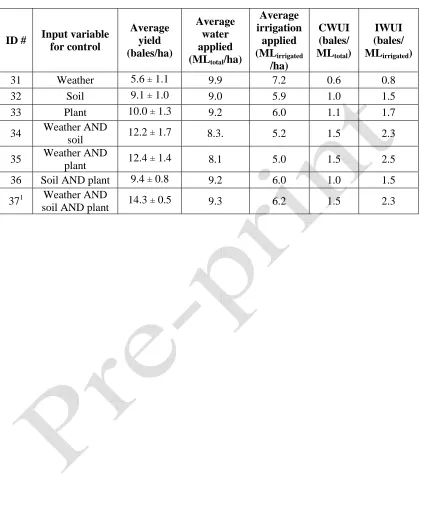
with different combinations of input data to calibrate RefModel. The use of more 531

information in the input data combination generally increased the average yield and 532

water use efficiency (Table 4). Table 4 shows that MPC performance with all three 533

input variables (simulation #37/#28) was superior to that with any two variables 534

(simulations #34-#36); and similarly performance with two input variables was 535

superior to that with any single input variable alone, except plant input (simulation 536

#33) versus soil-and-plant input (simulation #36). This suggests that the MPC 537

calibration performs better with soil data input than plant data input. 538

539

(23)

23

The lowest yields and water use efficiencies were simulated with only weather data 543

input (e.g. simulations #31). This is because the weather data (without field-specific 544

soil or crop data) provides no information to adequately parameterise the crop model 545

used by the MPC strategy. This could lead to insufficient model calibration and sub-546

optimal irrigation volumes being determined. The irrigation water use efficiency was 547

higher using the weather and plant combination (simulation #35) than using the full 548

data input (simulation #37/#28): this is because the yield was maximised rather than 549

the water use efficiency in this case study. 550

551

6. GENERAL DISCUSSION 552

A Model Predictive Control strategy was successfully implemented in VARIwise. 553

The controller uses currently available field data to calibrate the OZCOT cotton 554

production model and then evaluates a range of irrigation volumes and timings in each 555

zone. The controller then implements the site-specific irrigation volumes on the day 556

that achieves the highest water use efficiency or yield averaged over the field, as user 557

specified. 558

559

Three alternative optimisation possibilities were identified and explored, and the 560

conclusions for each, and their comparison, are as set out below. In each case the 561

MPC strategy performed successfully in the (simulated) task of controlling an 562

automatic irrigation machine applying spatially-varied irrigation amounts. For 563

convenience, Table 5 gathers together the particular simulation outputs referred to in 564

this section. Table 5 also compares results of MPC with two sensor-based control 565

strategies, namely Iterative Learning Controller (ILC) and Iterative Hill Climbing 566

(24)

24

with 1266 zones, and the same weather profile and crop variety (as detailed in 568

McCarthy et al. 2013). These sensor-based strategies refine the estimate of each 569

successive irrigation volume applied by: 570

[ILC] – iteratively adjusting the irrigation volume applied in each zone of the field 571

using the incremental response, i.e. the OZCOT-determined plant growth arising 572

from the change in particular field sensor information which has resulted from the 573

previous water application, in each zone; or 574

[IHCC] – similarly adjusting the irrigation volumes, but based on multiple sensor 575

increment information, using a range of irrigation volumes applied within a group 576

of homogenous zones. 577

578

580

The performance of the MPC strategy was also compared with an industry-standard 581

irrigation strategy (first line of Table 5). This strategy applied a uniform irrigation 582

treatment (25 mm) across the field and initiated irrigation events when the soil-water 583

deficit reached a set amount (30 mm) in one point in the field (in the cell with sandy 584

soil). The soil-water deficit was taken in the cell with the lowest plant available water 585

capacity, as this is the most limiting soil. To ensure validity of the comparison this 586

simulation was executed using the same weather conditions and spatially variable 587

plant available water capacity and starting soil-water, and crop variety as the reference 588

model. The nitrogen content was set to 250 kg/ha. 589

590

The MPC strategy was evaluated with different combinations of input data (section 3 591

(25)

25

maximised the square count and calibrated the model using all three streams of data 593

input (weather, soil and plant, simulation #20). The yield and water use efficiency 594

were also higher than those of the industry-standard irrigation management strategy 595

(McCarthy et al. 2013), and also ILC (simulation #1) and IHCC (simulation #9) with 596

either weather-soil-and-plant, weather-and-soil or weather-and-plant data input 597

available (likewise refer McCarthy et al. 2013). However, the MPC (optimising daily 598

input data) performed worse than the ILC and IHCC where there was only either soil 599

input (simulation #11) or weather-and-plant (simulation #14) input data available. 600

601

The controller successfully adjusted the irrigation to improve the yield, CWUI or 602

IWUI, as appropriate (Section 4). The yield was higher with high nitrogen content 603

(e.g. simulation #28) than with low nitrogen content (simulation #25) and with no 604

rainfall during the crop season (simulation #23) compared with high rainfall 605

(simulation #28). This is because the control strategy could better control the water 606

applied in response to the other environmental factors. The simulated average yields 607

and water use efficiencies were significantly higher than the industry-standard 608

irrigation management strategy, ILC strategy (simulation #1) and IHCC strategy 609

(simulation #9) (McCarthy et al. 2013). 610

611

MPC was evaluated with different combinations of input data available to calibrate 612

the model (Section 5). The controller performed best with input of weather-soil-and-613

plant data (simulation #28), but still produced higher yields and water use efficiencies 614

with weather-and-soil (simulation #34) or weather-and-plant (simulation #35) input 615

than the irrigation-standard irrigation management strategy, and ILC (simulation #1) 616

(26)

26 618

Higher yields and water use efficiencies were produced for MPC optimising predicted 619

end-of-season data (simulation #28) than for MPC using daily input data to maximise 620

square count (simulation #20). However, both of these control strategies required 621

either the full data input, weather-and-soil or weather-and-plant data input to obtain 622

yields higher than the ILC or IHCC strategies. 623

624

7. CONCLUSION 625

The Model Predictive Control strategy implemented in the control simulation 626

software VARIwise performed successfully in the task of controlling an automatic 627

irrigation machine applying water to a simulated cotton crop grown in typical 628

conditions for south-east Queensland, Australia. In all simulations the MPC strategy 629

specified ‘sensible’ irrigation amounts typical of irrigation practice in this region. 630

Simulations using the MPC strategy indicated that the MPC strategy could be 631

successfully used to either maximise crop yield, or crop and irrigation water use 632

efficiencies. 633

634

The MPC strategy produced significantly higher yield and crop water use efficiency 635

than the sensor-based strategies for the same (simulated) field conditions (similarly 636

simulated in VARIwise and reported in McCarthy et al. 2013). However, MPC 637

required weather-soil-and-plant, weather-and-soil or weather-and-plant information to 638

accurately calibrate the crop model. This indicates (for cotton grown as stated) that 639

whilst the MPC-based strategies are potentially superior, sensor-based strategies may 640

be more appropriate for field implementations where there is limited data availability. 641

(27)

27

Finally, we note here that direct field evaluation is particularly challenging, because 643

direct comparison requires replicated plots having the same soil types and 644

distributions, and with simultaneous operation such that each experiences the same 645

weather conditions. In principal at least, an alternative to achieve such a comparison 646

would be to determine variability of soil properties under an irrigation system, a 647

priori, and then define plots of the same soil type such that the irrigation application 648

could be adjusted according to different MPC strategies, and in comparison with 649

industry-standard control (e.g. calculated using evapotranspiration or soil-water). 650

651

Field evaluations would enable the sensing and control hardware requirements and 652

performance of autonomous, adaptive control strategies to be compared with industry-653

standard irrigation. These control strategies would determine irrigation application 654

and timing using a black-box control system based on sensed inputs and sends control 655

signals to irrigation actuation hardware. This will potentially lead to the optimisation 656

of irrigation water use and yield under different climate scenarios and water 657

availability situations. 658

659

Acknowledgements 660

The authors are grateful to the Australian Research Council and the Cotton Research 661

and Development Corporation for funding a postgraduate studentship for the senior 662

author; and to the anonymous reviewers for suggestions concerning potential field 663

evaluation. 664

665

(28)

28

CSD (2009) Cotton Seed Distributors Ltd. Viewed 10 December 2009, 667

http://www.csd.net.au/. 668

669

Ebert, EE (2001) Ability of a poor man’s ensemble to predict the probability and 670

distribution of precipitation. Monthly Weather Review 129:2461-2480. 671

672

Kwon, W. and Han, S. (2005) Receding horizon control: model predictive control for 673

state models. Advanced textbooks in control and signal processing, Springer-Verlag, 674

London. 675

676

Maciejowski, J.M. (2002) Predictive control with constraints. Pearson Eduation 677

Limited, Essex. 678

679

McCarthy, A.C., Hancock, N.H. and Raine S.R. (2010a) VARIwise: a general-680

purpose adaptive control simulation framework for spatially and temporally varied 681

irrigation at sub-field scale. Computers and Electronics Agriculture 70(1):117-128. 682

683

McCarthy, A.C., Hancock, N.H. and Raine, S.R. (2010b) Simulation of site-specific 684

irrigation control strategies with sparse input data. In: CIGR 2010: Sustainable 685

Biosystems Through Engineering, 13-17 June 2010, Quebec City, Canada. 686

687

McCarthy, A.C., Hancock, N.H. and Raine, S.R. (2011) Real-time data requirements 688

for model-based adaptive control of irrigation scheduling in cotton. Australian 689

Journal of Multi-disciplinary Engineering 8(2):189-206. 690

(29)

29

McCarthy, A.C., Hancock, N.H. and Raine, S.R. (2013) Development and simulation of 692

sensor-based irrigation control strategies for cotton using the VARIwise simulation 693

framework. Submitted to Computers and Electronics in Agriculture 694

695

Park, Y., Shamma, J. and Harmon, T. (2009) A receding horizon control algorithm for 696

adaptive management of soil moisture and chemical levels during irrigation. 697

Environmental Modelling and Software 24(9):1112-1121. 698

699

QNRM (2009) Queensland Natural Resources and Mines enhanced meteorological 700

datasets. Viewed 4 March 2008, http://www.longpaddock.qld.gov.au/silo/. 701

702

Richards, Q., Bange, M. and Roberts, G. (2001) Assessing the risk of cotton 703

‘earliness’ strategies with crop simulation. In: ‘Proceedings of the 10th Australian 704

Agronomy Conference’, The Australian Society of Agronomy, Hobart. 705

706

Wells, A. and Hearn, A. (1992) OZCOT: a cotton crop simulation model for 707

(30)

30 Figures and Tables

[image:30.595.98.494.181.651.2]

709 710

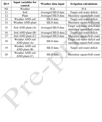
Table 1: Simulations (identified by ID #) conducted to compare interactions between 711

control strategies and input variables for Model Predictive Control. N/A indicates 712

non-applicable and SILO indicates use of historical climate data. (Simulations #1 to 713

#10 not tabulated here are those undertaken for sensor-based control, McCarthy et al. 714

(2013).) 715

716

ID # Input variables for

control Weather data input Irrigation calculations

Nil Weather N/A N/A

11 Soil Averaged SILO data Target soil-water deficit 12 Plant Averaged SILO data Maximise square/boll count 13 Weather AND soil SILO data Target soil-water deficit 14 Weather AND plant SILO data Maximise square/boll count 15 Soil AND plant (A) Averaged SILO data Target soil-water deficit and maximise square/boll count 16 Soil AND plant (B) Averaged SILO data Target soil-water deficit 17 Soil AND plant (C) Averaged SILO data Maximise square/boll count 18 Weather AND soil

AND plant (A) SILO data

Target soil-water deficit and maximise square/boll count 19 Weather AND soil

AND plant (B) SILO data Target soil-water deficit 20 Weather AND soil

(31)

[image:31.595.65.517.98.638.2]

31

Table 2: Performance of the model predictive control strategy with variable-rate 717

irrigation machine for different input data combinations (yield maps of simulations 718

#11-#20 are in Figure 3) 719

720

ID #

Input variable for control

Average yield (bales/ha)

Average water applied (MLtotal/ha)

Average irrigation

applied (MLirrigated/ha)

CWUI (bales/ MLtotal)

IWUI (bales/ MLirrigated)

11 Soil 5.2 _± 2.4 9.4 6.4 0.5 0.8

12 Plant 2.9 _± 2.1 4.6 1.5 0.6 1.9

13 Weather AND

soil 7.4 ± 1.5 9.2 6.2 0.8 1.2

14 Weather AND

plant 6.4 ± 1.0 5.3 2.2 1.2 2.9

15 Soil AND plant

(A) 7.8 ± 1.9 8.8 5.7 0.9 1.4

16 Soil AND plant

(B) 7.3 ± 2.1 9.5 6.4 0.8 1.1

17 Soil AND plant

(C) 8.2 ± 2.7 9.0 5.9 0.9 1.4

18

Weather AND soil AND plant

(A)

10.8 ± 1.6 8.8 5.7 1.2 1.9

19

(B)

10.6 _±1.9 10.2 7.1 1.0 1.5

20

(C)

(32)

32

Table 3: Performance of the model predictive control strategy with variable-rate 721

irrigation machine for different weather data inputs, starting nitrogen contents and 722

optimised variables (yield maps of simulations #21-#30 are in Figure 6) 723

724

ID #

Optimised variable

Rainfall (mm)

Initial nitrogen

content (kg/ha)

Average yield (bales/

ha)

21 Yield 0 120 9.0 _± 0.4 6.8 6.8 1.3 1.3

22 CWUI/Yield 0 120 8.4 _± 0.6 5.2 5.2 1.6 1.6

23 Yield 0 250 17.9 ±

0.9 6.6 6.6 2.7 2.7

24 IWUI/Yield 0 250 17.3 ±

1.2 6.5 6.5 2.7 2.7

25 Yield 302 120 8.4 ± 0.4 9.0 5.9 0.9 1.4

26 CWUI 302 120 8.4 ± 0.6 8.1 5.0 1.0 1.7

27 IWUI 302 120 7.7 _± 0.5 7.5 4.4 1.0 1.8

28 Yield 302 250 14.3 ±

0.5 9.3 6.2 1.5 2.3

29 CWUI 302 250 13.3 ±

1.0 7.8 4.7 1.7 2.8

30 IWUI 302 250 12.5 ±

(33)

[image:33.595.89.512.133.665.2]

33

Table 4: Performance of the model predictive control strategy optimising yield for 725

crop season with rainfall and 250 kg/ha of available nitrogen for different input data 726

combinations, where simulation #371 is a duplication of simulation #28 for 727

comparison (yield maps of simulations #31-#37 are in Figure 9) 728

729

ID # Input variable for control

Average yield (bales/ha)

applied (MLirrigated

/ha)

31 Weather 5.6 ± 1.1 9.9 7.2 0.6 0.8

32 Soil 9.1 ± 1.0 9.0 5.9 1.0 1.5

33 Plant 10.0 _± 1.3 9.2 6.0 1.1 1.7

34 Weather AND

soil 12.2 ± 1.7 8.3. 5.2 1.5 2.3

35 Weather AND

plant 12.4 ± 1.4 8.1 5.0 1.5 2.5

36 Soil AND plant 9.4 ± 0.8 9.2 6.0 1.0 1.5

371 Weather AND

(34)

34

Table 5: Control strategy simulation outputs where the initial nitrogen content is 250 730

kg/ha and there is rainfall during the crop season unless otherwise noted. 731

732

ID # Control strategy Input variable for control Average yield (bales/ha) Average water applied (MLtotal/ha)

N/AA

Industry-standard Nil 9.1 ± 1.9 10.2 6.8 0.9 1.4

1A ILC Soil 12.2 _± 1.5 11.0 7.3 1.1 1.7

9A IHCC Soil AND

plant 12.4 ± 1.6 12.2 8.1 1.0 1.5

11 MPC (daily

input) Soil 5.2 ± 2.4 9.4 6.4 0.5 0.8

14 MPC (daily input)

Weather AND plant

6.4 _± 1.0 5.3 2.2 1.2 2.9

20 MPC (daily input)

Weather AND soil

AND plant

12.1 ± 0.7 9.4 6.3 1.3 1.9

23 MPC (end- of-season input)1

Weather AND soil

AND plant

17.9 _± 0.9 6.6 6.6 2.7 2.7

25 MPC (end- of-season input) 2

Weather AND soil

AND plant

8.4 ± 0.4 9.0 5.9 0.9 1.4

28/ 37

MPC (end- of-season input)

Weather AND soil

AND plant

14.3 ± 0.5 9.3 6.2 1.5 2.3

34 MPC (end- of-season input)

Weather

AND soil 12.2 ± 1.7 8.3 5.2 1.5 2.3

35 MPC (end- of-season input)

Weather AND plant

12.4 _± 1.4 8.1 5.0 1.5 2.5

A

From McCarthy et al. 2013

733

1

Crop season has no rainfall

734

2_{Initial nitrogen content is 250 kg/ha}

735

Abbreviations: ILC is Iterative Learning Control, IHCC is Iterative Hill Climbing Control and MPC is

736

Model Predictive Control

(35)

35 738

[image:35.595.89.510.68.315.2]

739

Figure 1: The simulation framework VARIwise configured to evaluate (in simulation 740

mode) the model-based adaptive control strategy Model Predictive Control (MPC). In 741

this mode, the block ‘AcModel’ (also an OZCOT formulation) has replaced the field 742

data measurements which would normally update ‘RefModel’. (This diagram is 743

adapted from the full VARIwise flowchart presented as Figure 2 of McCarthy et al. 744

(36)

36 746

(a) 747

748

749

(b) 750

[image:36.595.113.480.70.679.2]

751

Figure 2: Soil variability as calibrated in model predictive control implementation: (a) 752

(37)

37 754

[image:37.595.115.482.68.709.2]

755

Figure 3: Yield maps and average yield and irrigation outputs of model predictive 756

control strategy for different combinations of data input and legend for yield maps for 757

(38)

38 759

(a) (b)

[image:38.595.93.489.72.284.2]

760 761

Figure 4: Simulated daily soil-water deficit in sand, clay loam and clay zones for 762

strategies that use weather, soil and plant data for model calibration (RefModel). Set 763

(a): targeting fixed soil-water deficit (simulation #19); and set (b): maximising 764

(39)

39 766

(a) (b)

[image:39.595.105.487.78.284.2]

767 768

Figure 5: Simulated daily square count in sand, clay loam and clay zones for strategies 769

that use weather, soil and plant data for model calibration (RefModel). Set (a): 770

targeting fixed soil-water deficit (simulation #19); and set (b): maximising square 771

(40)

40 773

[image:40.595.114.479.68.704.2]

774

control strategy with variable-rate irrigation machine and legend for yield maps for 776

(41)

41 778

(a) 779

780

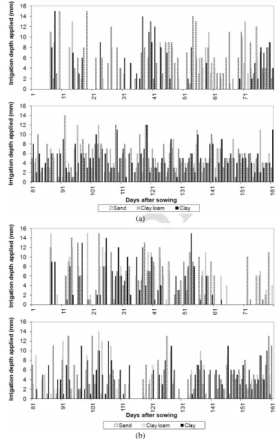
[image:41.595.94.496.73.709.2]

(b) 781

Figure 7: Irrigation volumes applied to sand, clay loam and clay zones for simulations 782

#24 and #27 to evaluate effect of rainfall during crop season. The model predictive 783

controller optimised IWUI with 250 kg/ha of available nitrogen and for crop season 784

(42)

42 786

(a) 787

788

789

[image:42.595.81.495.67.711.2]

(b) 790

Figure 8: Irrigation volumes applied to sand, clay loam and clay zones for simulations 791

#25 and #28 to evaluate effect of nitrogen content; the model predictive controller 792

optimised yield for crop season with no rainfall and available nitrogen of: set (a) 120 793

(43)

43 795

[image:43.595.90.508.71.612.2]

796

control strategy with variable-rate irrigation machine and legend for yield maps, 798

where simulation #371 is a duplication of simulation #28 for comparison (numerical 799