Multi Reservoir Water Price and Allocation Model

(1)

International Journal of Innovative Technology and Exploring Engineering (IJITEE) ISSN: 2278-3075, Volume-9 Issue-1, November 2019

2220

Published By:

Blue Eyes Intelligence Engineering & Sciences Publication

Retrieval Number: A4789119119/2019©BEIESP DOI: 10.35940/ijitee.A4789.119119



Abstract: Many water planning, researches have been done but water pricing has not been considered as the prime factor. Cost allocation is required whenever a project deals with multi-purpose groups. An optimization model which is accommodating the water allocation and water price must be developed in Indonesia. The new linear optimization model is developed to present a method for the determination of equitable impact fees and optimal water allocation for single reservoir. The proposed method is demonstrated on a river system with 4 major reservoirs. Each reservoir system serves 5 uses (irrigation, hydroelectric and flood control, industrial and domestic need). Using optimization with the cost of the reservoir and its facilities as targets and the objective function is maximization of total net benefit of user income, water allocation as x variable and water price as the y variable will produce the optimal result. The result is the optimal water allocation with a minimal water price which is present on 3 simulation analysis. The result of the model is in a graphic and table presentation, which can be used easily to determine the water allocation and water price per m3 in all reservoir systems.

Keywords : Allocation, Model, Optimization, Water Price.

I. INTRODUCTION

Water is the source of life, whose existence is absolutely necessary. In in today modern life, the role of water is absolutely important. Civilization grew, starting from the industrial revolution in the eighteenth century. Likewise civilization in the field of water. Water problems faced by human life are increasing, but there is still a lot of technologies to overcome this water problem. Today's water needs are not only for agriculture, household and transportation lines, but also for energy generation, industrial processes and commercial purposes.

The older the world the higher the global temperature increase. It reflects to the rain water volume decrease [1].

The international meeting of the UNED agency of the United Nations in 1996 reviewed the relationship between regulating water through economic mechanisms. This meeting resulted in the principle that water is an economic commodity and needs a program and clear rules for allocation and payment according to its value. The policy of paying for water costs must be carried out in accordance with the arrangements to obtain a sustainable distribution of water [2]. The Law of the Republic of Indonesia Number 7 of 2004

Revised Manuscript Received on November 05, 2019. * Correspondence Author

Rispiningtati*, Water Resources Engineering Department, Engineering Faculty, Brawijaya University, Malang, Indonesia. Email: rispiningtati@ub.ac.id

Rudy Soenoko, Mechanical Engineering Department, Engineering Faculty, Brawijaya University, Malang, Indonesia. Email: rudysoen@ub.ac.id

concerning Water Resources, also states the need for a new paradigm in water resources management with adaptive modern management behavior. Water is an economic commodity [3]. The importance of optimizing water prices based on needs and regulating water requirements affecting the amount of water prices [4]. Water resources management must go through the Hydro Politic approach where the policy of water management is not just setting the amount or volume of water, but financed is a factor that must not be ignored [5]. Water is an economic commodity which cost of water consisted of distribution, production and transmission [6], [7]. Water cost optimization is based on the demand and regulation of water need allocation [8], [9]. Many research was conducted about water allocation optimization without water cost [10], [11], [12].

Several opinions above would be the base of estimating the cost and allocation of water research. For the meantime the optimization study of water cost and allocation simultaneously is not being conducted yet. So the gap in the old research is the optimization is just for the allocation only without any consideration of water cost.

The research considered necessary, is the regulation of water allocation at river systems with water as an economic commodity. To get the allocation regulation and water cost appropriately, the new optimization model must be conducted. The new model be used in this research is applied to the Brantas River in East Java Indonesia. The new model will optimize the water allocation together with the water cost. To show the new and old model, it can be seen in the example bellow. The model is used to regulate the multifunction reservoir. The reservoir has 5 functions; the first is the Irrigation (y1x1); second is the Hydropower (y2x2); third is the Flood Control (y3x3); forth is the Industry (y4x4); and the fifth is the Domestic Water (y5x5).

To get the allocation rules and certainty of water prices, a method based on the optimal approach is needed. Optimization method works with the principle of optimizing an objective function against constraints.

II. MATERIAL AND METHODS A. Regular Model Objective Function

Max Z (Income);

y1x1 + y2x2 + y3x3 + y4x4 + y5x5 (1) The constraints are; x1, x2, x3, x4, x5 ≥ User need (Constrain volume); x1, x2, x3, x4, x5 ≤ Reservoir Capacity; y1, y2, y3, y4, y5 = Unit Cost of Water or x coefficient; x1, x2, x3, x4, x5 → are variables.

Multi Reservoir Water Price and Allocation

Model

(2)

2221

Published By:

B. The Research Model Objective Functions

Maximize x and Minimize y;

z = y1x1 + y2x2 + y3x3 + y4x4 + y5x5 (2) The constraints are; x1, x2, x3, x4, x5 ≥ User need (Constrain Volume); x1 + x2 + x3 + x4 + x5 ≤ Reservoir Capacity; y1, y2, y3, y4, y5 = Water Variable Cost; x1, x2, x3, x4, x5 → Water allocation variables

The program is required to optimize the water allocation unit and the water price. The difference between the regular and research model could be seen in Fig. 1 and Fig. 2.

Fig. 1. Regular Model Flow Chart

Fig. 2. Research Model Flow Chart

C. The Research or Water Allocation and Price Model

There are several studies on water rates or prices, but are not an integrated unit of allocation and price for all river systems, such as a simulation study of the water price system for efficient use of domestic water (drinking water) [12]. According to the research, the price of water is determined based on the criteria of water availability. If abundant water is

low in price, if the water is reduced is subject to high prices, where the volume and price are determined by simulation.

Optimization studies that have been carried out in Indonesia are only for water allocation, there has not been a comprehensive study of water prices in a river system [13]. Some water allocation studies present a water allocation model for applications in Indonesia such as WRMM (Water Resources Management Model) originating from Optimal Solution Ltd. Alberta Environment Canada is applied for Study of River Areas in Ciujung, Cimanuk-Cisanggarung, Progo-Opak-Oya, Ciliman, Jratunseluna and Pekalen Sampalen. This model specifically discusses the policy of water allocation by limiting the water need and availability, the component of water prices has not been used as a basis for policies. So the model produced is an WRMM application package program made from outside Indonesia and is not a program produced in Indonesia.

Some explanation requires about phrases used in the model such as:

 Water Allocation is a control of water volume to distribute water to water users [14].

 Water price is the price of each unit of water that is distributed to water user [15], [16].

 Water users are the Irrigation, Hydropower, Flood control, Industrial, Domestic water, Flashing need [17].

 Irrigation user is a unit volume water that could be distributed in the irrigate farm area.

 The Hydropower user is the water unit volume to produce electric energy.

 The Flood control user is the water volume that must be retarded to cope flooding of the dam or reservoir down-stream area.

 Industrial water is specified as water volume use for lake recreation such as boating, surfing. Fishery and others [18].

 Domestic Water is the unit volume of water use for public need [19].

 Flushing Water is the water volume that should always be on the river or base flow.

The new model as the tool is used to find the optimal solution. Start the process with the mathematical model to be answered (a) What variables or unknown factors that must be found; (b) What constrains that required to optimize the process; (c) What are the objective functions to gain the best result.

The river manager will determine the water volume amount required or discharge to be drawn from each reservoir at the river system. To draw the water volume amount there is a calculation as an economic allocation to get a maximal income, on the other hand the user-need abundant water with a minimal price [20]. For example; the reservoir has 6 million m3storage at the first semester and 8 million m3 at the second semester [21]. The Irrigation required two times amount of water than the Hydro power does at the first semester. At the second semester Hydro power require two times more than the irrigation requirement. Hydropower required a one million m3 more than the irrigation requirement. Hydropower requirement should always

(3)

2222

Published By:

1 (

)

n

i

TNB

B

y x







irrigation, in the Indonesian Dollar thousand (IDR), is two and three for the Hydropower.

To solve the problem, there are some variables to be considered, which is

(a) The variable: x1 = irrigation requirement; x2 = Hydropower requirement;

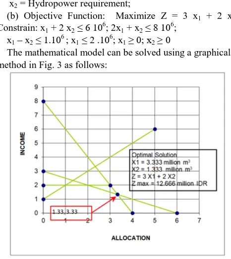
(b) Objective Function: Maximize Z = 3 x1 + 2 x2; Constrain: x1 + 2 x2 ≤ 6 106; 2x1 + x2 ≤ 8 106;

x1 – x2 ≤ 1.106 ; x1 ≤ 2 .106; x1 ≥ 0; x2 ≥ 0

[image:3.595.50.283.115.376.2]

The mathematical model can be solved using a graphical method in Fig. 3 as follows:

Fig. 3. Graphical Optimization solution

The graphical method shows the optimal solution related to the extreme point. For example, for two variables it should have more than two variables. It should be better to use the Simplex Method in Linear Programing [22], [23], [24].

D. Water Allocation and Water Price Model

The optimization model in this study is a deterministic mathematical model with the aim of optimal solving, the testing method is not suitable for systems that do not yet exist, so the test is only a comparison with other mathematical models [25]. To meet the criteria for a comprehensive optimization study containing elements of the allocation along with the value of water, the optimization of the description consists of three stages:

 Optimization of allocations with reservoir outflow optimization.

 Optimize prices by meeting reservoir cost targets and facilities and maximize user income.

 Post optimization analysis by regressing the optimal allocation and price so that form an equation that can be used as a benchmark for water prices.

The Objective Function is to maximize x and minimize y:

(3)

If n = 5 then TNB = (B1 - y1)x1 + (B2 – y2)x2 + (B3 – y3)x3 + (B4 – y4)x4 + (B5 – y5)x5; The variables are; -y1, y2, y3, y4, y5; (WaterPrice); - x1, x2, x3, x4, x5 (Water Allocation)

The constraints are; z = y1x1 + y2x2 + y3x3 + y4x4 + y5x5 (Target); x1, x2, x3, x4, x5 … ≥ Requirement (Volume Constraints); x1 + x2 + x3 + x4 + x5 ≤ Reservoir Capacity (Volume Constraints); y1, y2, y3, y4, y5 ≤ Decision Ratio; B1,

B2…..B5 = income per m3_{; Z = Target (Cost of Reservoir and} its facility); TNB = Total Net Benefit

E.Reservoir Allocation Optimization

Reservoir outflow optimization is a reservoir outflow optimization arrangements to produce maximum benefits, especially in multi-purpose annual reservoirs whose optimization role are very important [26], [27]. The reservoir outflow optimization completion of this model is using a program solver which essentially maximizes the reservoir outflow amount with the limit of storage volume and the amount of the user needs. The solver program has advantages in the optimization process, the optimization process time is shorter than other optimization programs [28].

The purpose of optimization of reservoirs that have hydropower facilities:

Purpose Function:

Max E = E1 + E2 + E3 + E4 + E5 ………… .En Obstacles :

Smin <Sn <Smax

Turbine outflow> Q downstream

One year total outflow = One year total inflow Where:

E = Energy per year (KWH) E = 9.8 e Q H x time

9.8 = gravity number (m/sec2) e = turbine and generator efficiency Q = turbine inlet (m3/sec)

H = hydropower effective Head (m) Time = hour

E1, E2, E3, ……… En = Monthly energy. Sn = Monthly pool (m3)

S min = minimum storage (m3) S max = maximum storage (m3)

Turbine out flow = Hydroelectric discharge (m3/sec) Q downstream = discharge in downstream reserv. (m3/sec) For daily reservoirs that do not function to store water, the purpose of the optimization is somewhat different because at any time the inflow value is assumed to be the same as the outflow value.

F. Basic Water Price Optimization Policy

The basic price optimization policy is the planned limit to meet the three optimization constraint criteria. This criterion is a presentation of several options to give a freedom to the model users.

 Water prices determination is according to the economic law which adheres to lower prices for more goods [29]. The pricing determination policy for model 1, is according to the economic law, which is the water consumption at a lower price than those who take less water. The policy criterion is translated as the price rises for less usage.  Water prices determination based on the environmental law

to preserve the increasingly limited presence of water [30]. According to the environmental law, model 2 takes a higher water price policy for taking a larger water collection. The policy can be translated with the price criteria increasing for greater needs.

(4)

2223

Published By:

proportional to the user income. If the user income is higher than the water price is higher too. So if the user income is smaller, then the water price is also low [31]. This policy for model 3 is translated as determining water prices and allocating water comparable benefits (income).

The policy that contains the three main bases of the optimization model is an obstacle in the element of price optimization. This basis is then processed in the form of a ratio or number of conversions to the program built so that the model requirements can be met.

G. The Decision Ratio

The boundary meets three constraints based on the of Water Price Optimization decision. The constraints are:

 Price Increase in less water utilized.  More water utilized more water price.

 The water price increase when the benefit is higher.

H. Regression Analysis

The regression analysis applied to show the relation between water allocation and price easier. The three non-linear equation convert to linear equation that is:

Power equation:

y =  x (4)

This equation can be expressed in a logarithmic equation Log Ŷ = log  -  log x. This term is a linear function in log x with variable: y = log ; x = log x. The non-linear regression turn into linear regression: y = arc log  x; where  = 1/n ∑ yi - / n ∑ xi = ỹ - x;  = (∑ xi yi - n x ỹ)/ (∑ xi2 – n x2); yi = Total price; xi = total allocation and n = sample amount. The regression effect y toward x can be obtained R2 = 1 – S2y/Sy2,

While: S2y = 1/ (n-2){ ∑n (yi - ỹ)2 - ß ∑n (xi-x)2 }; Sy2 = 1/(n-1) ∑n (yi - ỹ)2

If the R2 value is approaching to 1 then all data would comprise in the regression equation.

Exponential equation:

y =  ex (5)

This equation is changing to Lne equation to be Ln y = Ln  - x Ln e. This form as a linear function in Ln e, with variable y = Ln y; x = x; The non-linear equation is turned into linear equation y = arc ln  ex; ,  , R2 be obtained equal to the power equation:

The Logarithm equation:

y =  log x + ; (6)

This term be converted to linear equation; the variable y = y and x = log x; ,  , R2 be obtained equal the power equation is the prevailing drag form at supersonic speeds, careful selection of the nose and tail shapes is mandatory to ensure performance and operation of the over-all system.

III. RESEARCH METHODE MODEL STRUCTURE

This research is model making that requires computer equipment and soft programs. Data needed include data on reservoirs along the Brantas River such as reservoir inflow and outflow data, reservoir technical data (maximum and minimum reservoir reservoir capacity, flood elevation, lowest water elevation, inundation area, high fall PLTA), irrigation area data (area, discharge planting needs). Data on reservoir costs, benefits (irrigation), hydropower, flood control,

industry, drinking water. The data obtained is directly there which also needs to be analyzed or calculated before entering into the optimization program.

Direct data include: Map of study area and reservoir location, debit data, technical data, total reservoir cost data, irrigation area data. Data analyzed or calculated: Hydropower needs and benefits, irrigation needs and benefits, flood control needs and benefits, drinking water needs and benefits and annual reservoir costs.

Brantas River has 4 single reservoir with every reservoir has users such as Irrigation, Hydropower, Flood Control, Domestic Water and Industry. The research applied to four single reservoirs which are the Sengguruh, Wonorejo, Selorejo and Bening reservoirs.

The Two Steps optimizations are the Outflow optimization and the Price optimization. Every reservoir has a different function as a yearly or daily reservoir. Yearly reservoir has a large reservoir it can store a year water inflow (discharge). Daily reservoir has a small reservoir it can just store a one of water inflow (discharge). At Brantas River there are four yearly reservoirs which are Sutami, Wonorejo, Selorejo, Bening and the rest are as daily reservoirs. The Brantas river single scheme could be seen in Fog. 4.

Fig. 4. Brantas River Single Reservoir Scheme A. Constraints Determination

(5)

2224

Published By:

B. Model Structure Planning

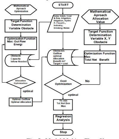
[image:5.595.56.256.88.320.2]

The research system is making and designing the model as in the flowchart in Fig. 5.

Fig. 5. Model Making Flow Chart

Optimization of a single reservoir if it is not related to other reservoirs, the Maximize Total Net Benefit of each user Max TNB = ∑n

i =1 (Bi-yi) yi, n = 5

Constrain: xi ≥ Water Volume requirement; ∑ ni =1 xi ≤ Water volume regulation; yi….≤ ratio model; Bi = Benefit per m3; Z =∑ ni =1 xi yi; Z = Total cost of the reservoir.

Price regulation depends on mutual agreement between managers and users. In accordance with the timing of debits calculated in the annual period, all components related to time

and costs are converted on an annual basis with a component of interest that is generally accepted in Indonesia (around 12%).

C. Multi Reservoir Constraints Arrangement

Water volume constraints that is complicated because of the large amount of related user water volume. The discharge is always changing depending on the climate conditions [11]. The amount of discharge is interconnected between the user and reservoir withdraw. As at the reservoir scheme where downstream reservoir depend on upstream reservoir, small change at the upstream reservoir will change all distribution systems. The upstream discharge continuity formula = downstream discharge if no additional or minus at any time. The notation = ∑Qn inflow = ∑Qn outflow ( n = 1, 2………4).

The model determination with a single reservoir scenario as part of the multi reservoir. The operation model with a large reservoir at Brantas River must be a one packed plan it could not be separated. The accepted rule must be given to the user to cope water payment fairly. Cost component that is related to time in this research is applied for 12 % rate annually. The main constraints include the reservoir capacity, price rule which is summarized in Table- I.

Table- I. Constrain record (Objective Function) Max: TNB = ∑n

i =1 (Bi-yi) xi , n = 5

1 2 3 4 5

Res. Out flow User Requirement

Model I, Price Decrease, Alloc.Increase

Model II, Price Increase, Alloc. Increase

Model III, Price equates Benefit

Q1 ≥ ∑x11 +...x15 x11...x15≥ m11…m15 y11...y15 ≤ r11…r15 y121…y125≤ r121…r125 y131…y133 ≤ r131…r135 Q2 ≥ ∑x21+…x25 x21...x25≥ m21…m25 y21...y25 ≤ r21…r25 y221…y225 ≤ r221…r225 y231…y233 ≤ r231…r235 Q3 ≥ ∑x31 +...x35 x31...x35 ≥ m31…m35 y31...y35 ≤ r31…r35 y321…y325≤ r321…r325 y331…y333 ≤ r331…r335 Q4 ≥ ∑x41 +...x45 X41...x45 ≥ m41…m45 y41...y45 ≤ r41…r45 y421…y425≤ r421…r425 y431…y433 ≤ r431…r435 Note:

Title: Objective function of price optimization; Column 1: Outflow Total Volume ≥Total allocation; Column 2: Total Allocation ≥Total user requirement; Column 3: model I Price Decrease, Allocation Increase: Price <1st Coefficient Ratio Model; Column 4: model II; Price Increase, Allocation Increase: Price <2nd Coefficient Ratio Model; Colom 5: model III Price equates to Benefit: Price<3rd Coefficient Ratio Model.

Optimization of a single reservoir if it is not related to other reservoirs, the Maximize Total Net Benefit of each user Max TNB = ∑n

i =1 (Bi-yi) yi, n = 5

Constrain: xi ≥ Water Volume requirement; ∑ ni =1 xi ≤ Water volume regulation; yi….≤ ratio model; Bi = Benefit per m3; Z =∑ ni =1 xi yi; Z = Total cost of the reservoir.

D. Sengguruh Reservoir Constraints Arrangement

As mentioned above that water volume constraints that is complicated for a single reservoir for Sengguruh reservoir. Because of the large amount of related user water volume.

[image:5.595.74.512.458.582.2]

(6)

2225

Published By:

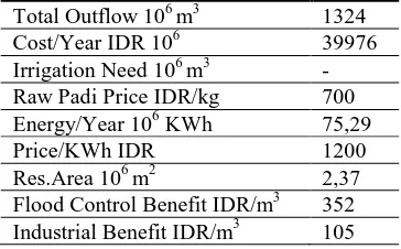
[image:6.595.78.260.177.290.2] [image:6.595.306.548.297.401.2]

The model determination should always refer to the single reservoir scenario as part of the multi reservoir. As mentioned before that at the Brantas River, as a large reservoir operation model, must determine as one packed plan, it could not be determined separately. The accepted rule must be given to the user to cope water payment fairly. The same value for the cost component related to time in this research is taken as big as the 12 % rate annually. The data constraints summarized for the Sengguruh reservoir could be seen d in Table- II.

Table- II. Data constraints (Sengguruh)

Total Outflow 106 m3 1324

Cost/Year IDR 106 39976

Irrigation Need 106 m3 -

Raw Padi Price IDR/kg 700

Energy/Year 106 KWh 75,29

Price/KWh IDR 1200

Res.Area 106 m2 2,37

Flood Control Benefit IDR/m3 352

Industrial Benefit IDR/m3 105

E. Reservoir Category

Single reservoirs consist of 4 reservoirs which are Sengguruh, Wonorejo, Selorejo, Bening. In this research case, the single reservoir chosen as the sample determination is the Sengguruh reservoir.

F. Model I: Price Decrease, Allocation Increase

The Model ratio number is the cost of the reservoir divided by the allocation times the constant.

Z / (xi * Bi) * C (7)

The water price y ≤ Ratio of each user; so y1 ≤ Z / x1 * B1*C; Z = Reservoir Annual Cost; x1 = User 1; B1= User 1 benefit per m3; C = conversion constant.

G. Model II: Price Increase, Allocation Increase

The ratio number for model II is the allocation time benefit divided by the average cost times the conversion constant.

The ratio number formula for Model II = xi * Bi / (Z / n) * C

For user 1:

y1 ≤ x1 * B1 / (Z/ n) * C;

x1 = User 1 allocation (m3); B1 = Benefit (IDR/m3); Z = Total cost of reservoir (IDR); n = user number; C = Conversion constant.

H. Model III: Price Equates to Benefit

The Model III Ratio Number is the allocation time benefit divided by the average allocation times total benefit times constant.

The Ratio number formula for Model III is: xi * Bi / ((∑ i1 xi) / i) * ∑ii Bi)) *C

For user 1 on the Reservoir that has 5 users: y1 ≤ x1 * B1 / ((∑i1 xi) / i * (∑i1 Bi)) * C Where: y1 is the Water Price per m

3

; B1 is the User 1 benefit (IDR/m3); (∑51x) / 5 is the average allocation (m3); ∑41B is the Total benefit (IDR/ m3); C is the Conversion constant.

IV. RESULT AND DISCUSSION

The optimization results in the form of the amount of water allocation and water price of each reservoir also are a result of overall optimization with three policies. This result is very useful if it can be used as a benchmark not only now but in the future. The form of a function in the form of a graph will be

more supportive for knowing allocations and prices and can be treated in general.

If the variable Y price function and variable X as an allocation function, the relationship between these functions is regressed to determine the correlation analysis between price and allocation in all cases. To sort out the optimal results in a coherent manner, the results are divided into 3 main relationships, namely:

 The relationship between the water allocation and water prices of all users for the entire system.

 The relationship between the user allocation and water prices in each single reservoir.

 The relationship between the water allocation and water prices of a group of users.

The users are the irrigation users, the hydropower benefit users, flood control, industry and drinking water. The example data for Sengguruh reservoir could be seen in Tabel- III.

Table- III. Model 1.1. Sengguruh Optimization result Optimization result

Total Net Benefit 53713 (106 IDR)

Users Allocation Price Power Exponent Log.

Hydro Power 1342 29 23 28 -10

Flood Ctrl. 1.42 320 223 132 256

Industrial 19 53 95 130 155

Total 1362 402 341 290 402

Average 454 134 114 97 32

The users are the irrigation users, the hydropower benefit users, flood control, industry and drinking water for sengguruh reservoir graph could be seen in Fig. 6.

Fig. 6. The relation between the water allocation and water price on Sengguruh Reservoir

Example: Water Allocation 106 m3, Water Price = IDR.50 / m3 The optimized result shows the water allocation and price of each reservoir with three categories. This result is useful to determine the minimal water price on the right allocation. The graphical presentation is easy to obtain the water allocation and its price. If y variable as price function and x variable as allocation function, then the relation between x and y has to be transformed into a regression function. Therefore the regression function shows the price and allocation correlation on all conditions.

The result of this simulation is to obtain a relationship between the allocation of water

[image:6.595.309.545.449.580.2]

(7)

2226

Published By:

The simulation results can be applied to every single reservoir along the Brantas river.

V. CONCLUSION

The Research Model has been made to optimize the water allocation and water price. The result that is the regression function relation between water allocation and price show the equation of the chosen model. x (106 m3) is the Water Allocation and y (IDR) is the Water Price/m3.

Variable factors taken into account in determining the value of water are obtained in a linear optimization model with the form of the objective function Max Z =  Xi Yi, which consists of variables X and Y where these two variables are greatly affecting the optimal results, for that in operation optimization of this model uses these two variables. Optimization of the old method is only an X variable that is optimized, so that the results are less optimal. Comparison of the optimization of the old and new methods applied to one of the reservoirs, with the same allocation (X = 270,106 m3), getting a new Y water price = IDR 48 / m3 smaller than the old Y water price = IDR 65 / m3. The new Y water price is more optimal because the value is smaller.

In studying and obtaining optimal allocation for users, the water allocation optimization model for each reservoir is to obtain the optimal water allocation result.

The development of an optimization model of water prices based on the prevailing policies and the amount of optimization of water allocation is to obtain three complete price simulations.

This model makes it easier to find out the optimal allocation and quantity of water prices using graphs or tables of the optimization results.

If the allocation and price optimization results stated in the regression equation, then the water allocation X is equal to 106 m3, the water price Y (IDR) = equal to water price / m3, the Z Total reservoir cost is equal to IDR 106, and the Total Net Benefits TNB is equal to IDR 106, the model results are Y = 250.88 X -0.3315 and Z = 39976; TNB = 53713, for the Sengguruh Reservoir. The Water Allocation and Price equation resume could be seen in Table- IV.

Table- IV. User Water Allocation and Price

User Price Equate To Benefit

Irrigation y = 0.0832 x 1.0049 Hydropower y = 0.5997 x 0.598 Flood Control y = 0.525 Ln (x) -0.0629 Industrial y = 0.1 x 0.5612 Domestic

Water

y = 0.308 x

REFERENCES

1. H. Cooley, N. Ajami, M. L. Ha, V. Srinivasan, J. Morrison, K. Donnelly, and J. C. Smith, “Global water governance in the twenty-first century. The World’s Water Volume 8. 2013.

2. J. J. Pigram, “Economic instrument in the management of australia’s water resources: A Critical View. International Journal of Water Resources Development. vol. 15 Issue 4, 2010, pp. 493-509; Published online: 21 Jul 2010.

3. D. Mc. Neill, “Water as an economic good”. Water Resources Update USA. 2000

4. J. A. Beecher, “Sustainable Water Pricing”, Water Resources Update 114: pp. 26-33. 1999.

5. D. Zaccaria, R. Maia, E. Vivas, M. Todorovic, A. Scardigno, “ Improving water-efﬁcient irrigation: Prospects and difﬁculties of innovative practices”, Agricultural Water Management 146 (2014), pp. 84–94.

6. DWR. Utah , “ The cost of water in Utah-Why are our water costs so low?“, Prepared by Utah Division of Water Resources, Salt Lake City, Utah 84114-6201, October 27, 2010.

7. EUWI, “Pricing water resources to finance their sustainable management”, A think-piece for the EUWI Finance Working Group. May 2012.

8. J. A. Beecher, “ Primer on water pricing”, Michigan State University; Institute of Public Utilities Regulatory Research and Education; November 1, 2011; ipu.msu.edu.

9. US, EPA. Planning for sustainability. A Handbook for Water and Wastewater Utilities, Prepared by Ross & Associates Environmental Consulting, Ltd. 1218 3rd Avenue, Suite 1207, Seattle, WA 98101 (206) pp. 447-1805, February 2012, EPA-832-R-12-001.

10. J.W. Labadie, Reservoir system optimization models. Water Resources Update, 2001, USA.108: pp. 83-110

11. M. L. Kansal and G. Arora, “Explore hybrid expert system for water network management”, American Society of Civil Engineers, ISSN (print): 0733-9496; ISSN (online): 1943-5452. 2001.

12. C. Leon, (2000). “Explore-hybrid expert system for water network management”, Journal of Water Resources Planning and Management, 126(2): 2000, pp. 65-75.

13. Rispiningtati, R. Soenoko, “Regulation of Sutami Reservoir to have a Maximal Electrical Energy”, International Journal of Applied Engineering Research. 10(12), 2015, pp. 31641-31648

14. P. D. Jankar, S. S. Kulkarni, “A case study of watershed management for Madgyal Village”, International Journal of Advanced Engineering Research and Studies, E-ISSN2249–8974, Int. J. Adv. Eng. Res. Studies/II/IV/July-Sept. 2013/69-72.

15. B. Sarah, The role of water pricing and water allocation in agriculture in delivering sustainable water use in Europe. Final Report, European Commission, Project number 11589, February 2012.

16. UNEP, Integrated water resources management planning approach for small island developing states. UNEP, 130 + xii, 2012.

17. L. A. M. John, The opportunity of crisis: A water reform agenda October 2012. The Australian Water Project, Volume 2. 2012. 18. F. Panahi, I. Malekmohammadim, M. Chizari, Jamal, M.V. Samani,

“The role of optimizing agricultural water resource management to livelihood poverty abolition in rural Iran”, Australian Journal of Basic and Applied Sciences, 2009, 3(4): 3841-3849, ISSN 1991-8178. 19. U. K. Shanwad, V.C. Patil, H. H. Gowda, G. S. Dasog and K.C.

Shashidhar, “Generation of water resources action plan for Medak Nala watershed in India using remote sensing and GIS technologies”, Australian Journal of Basic and Applied Sciences, 5(11): 2209-2218, 2011, ISSN 1991-8178.

20. P. H. Gleick, Water planning and management under climate change. The World’s Water, 2000, 112: pp. 25-32.

21. M. A. S. Tabieh, J. Suliman, A. Al-Horani, “Pricing mechanism as a tool for water policy using a Linear Programming Model”. Australian Journal of Basic and Applied Sciences, 4(8): 3159-3173, 2010 ISSN 1991-8178.

22. S. P. Saravanan, and R. Gobinath, “Drinking water safety through bio sand filter - A case study of Kovilambakkam Village, Chennai”, International Journal of Applied Engineering Research, ISSN 0973-4562 Vol. 10 No.53 (2015).

23. D. K. Nagesh, “Optimal reservoir operation for Irrigation of multiple crops using genetic algorithms”, Journal of Irrigation and Drainage Engineering© ASCE / March/April 2006 / 123.

24. M. J. Brown, Priority based reservoir optimization using Linear Programming: Application to the flood operation of the Iowa/Des Moines River System. B.S. (The Pennsylvania State University) 1995 Thesis Submitted in partial satisfaction of the requirements for the degree of Master of Science in Civil and Environmental Engineering; Committee in Charge 2005.

25. H. A. Taha, Operation Research. Second Edition. Department of Industrial Engineering of University of Arkansas. USA. 1996.

(8)

2227

Published By:

27. L. Lasdon, Microsoft Excel Solver uses the Generalized Reduced Gradient Non linear Optimization. University of Texas Austin Cleveland State University. 1998.

28. T. D. Tilahun Derib Asfaw, A. M. Hashim, “Reservoir Operation Analysis Aimed to Optimize the Capacity Factor of Hydroelectric Power Generation”, 2011 International Conference on Environment and Industrial Innovation; IPCBEE vol.12 (2011) © (2011) IACSIT Press, Singapore

29. I. Lippai, “Efficient and Equitable Impact Fees for Urban Water System”. Journal Of Water Resources Planning and Management, 2000. 126(2): pp. 75-84.

30. Mac. Donald, A. “Water Resources in Twenty First Century, A Global Challenge”. Journal of Comission Water Engineering Management, 2001, 15: pp. 157-161.

31. D. Mc. Neill, Water as an Economic Good. Water Resources Update USA. 2000.

AUTHORS PROFILE

Rispiningtati Rispiningtati is currently working as a lecturer in the Water Resources Engineering Department, Brawijaya University, Malang, Indonesia. She has completed her Doctor degree in Water Resources Engineering at the Brawijaya University, Malang, Indonesi (2006). Her Master degree in Water Resources Engineering was taken at the Manitoba University, Manitoba, Canada (1984). Her second Master degree is taken at The University of Melbourne, Melbourne, Australia (1992). She has been doing research in Water Resources Engineering, Water Resources Management, Electrical Engineering Water Power and Engineering Economic. She has total a Academic teaching experience of more than 40 years with many publications in reputed National and International E-SCI SCOPUS Journals, Taylor & Francis Springer, Elsevier Science Direct, She is also a member of various National and International professional societies in the field of engineering & research like Member of Indonesian Association of Hydraulic Engineers (HATHI).