Rhizosphere to the atmosphere: contrasting methane pathways, fluxes, and geochemical drivers across the terrestrial–aquatic wetland boundary

https://doi.org/10.5194/bg-16-1799-2019 © Author(s) 2019. This work is distributed under the Creative Commons Attribution 4.0 License.

Rhizosphere to the atmosphere: contrasting methane pathways,

fluxes, and geochemical drivers across the terrestrial–aquatic

wetland boundary

Luke C. Jeffrey1,2, Damien T. Maher1,2,3, Scott G. Johnston1, Kylie Maguire1, Andrew D. L. Steven4, and Douglas R. Tait1,2

1_{SCU Geoscience, Southern Cross University, P.O. Box 157, Lismore, NSW 2480, Australia}

2_{National Marine Science Centre, Southern Cross University, P.O. Box 4321, Coffs Harbour, NSW 2450, Australia} 3_{School of Environment, Science and Engineering, Southern Cross University, Lismore, NSW 2480, Australia} 4_{CSIRO Oceans and Atmosphere, Queensland Biosciences Precinct, University of Queensland, 306 Carmody Rd,} St Lucia, Brisbane 4067, Australia

Correspondence:Luke C. Jeffrey (luke.jeffrey@scu.edu.au) Received: 15 January 2019 – Discussion started: 22 January 2019

Revised: 29 March 2019 – Accepted: 2 April 2019 – Published: 29 April 2019

Abstract. Although wetlands represent the largest natural source of atmospheric CH4, large uncertainties remain re-garding the global wetland CH4flux. Wetland hydrological oscillations contribute to this uncertainty, dramatically alter-ing wetland area, water table height, soil redox potentials, and CH4emissions. This study compares both terrestrial and aquatic CH4 fluxes in permanent and seasonal remediated freshwater wetlands in subtropical Australia over two field campaigns, representing differing hydrological and climatic conditions. We account for aquatic CH4diffusion and ebulli-tion rates and plant-mediated CH4fluxes from three distinct vegetation communities, thereby examining diel and intra-habitat variability. CH4emission rates were related to under-lying sediment geochemistry. For example, distinct negative relationships between CH4fluxes and both Fe(III) and SO24− were observed. Where sediment Fe(III) and SO2₄−were de-pleted, distinct positive trends occurred between CH4 emis-sions and Fe(II)/acid volatile sulfur (AVS). Significantly higher CH4 emissions (p< 0.01) in the seasonal wetland were measured during flooded conditions and always dur-ing daylight hours, which is consistent with soil redox po-tential and temperature being important co-drivers of CH4 flux. The highest CH4fluxes were consistently emitted from the permanent wetland (1.5 to 10.5 mmol m−2d−1), followed by thePhragmites australiscommunity within the seasonal wetland (0.8 to 2.3 mmol m−2d−1), whilst the lowest CH4

fluxes came from a region of forestedJuncusspp. (−0.01 to 0.1 mmol m−2d−1), which also corresponded to the highest sedimentary Fe(III) and SO2₄−. We suggest that wetland re-mediation strategies should consider geochemical profiles to help to mitigate excessive and unwanted methane emissions, especially during early system remediation periods.

1 Introduction

wet-CH4 emissions (Wang et al., 1996; Whiting and Chanton, 2001). Mitsch et al. (2013) estimated that the average ra-tio of freshwater wetland CO2 sequestration to CH4 emis-sions was 25.5:1, though this was later refuted by Bridgham et al. (2014). As CH4 is 34 times more potent than car-bon dioxide (CO2) over a 100-year timescale (Stocker et al., 2013), this suggests that many freshwater wetlands may have a net positive radiative forcing effect on climate (Petrescu et al., 2015; Hemes et al., 2018). However, variability in morphology, wetland maturity, salinity, and underlying geo-chemical composition contributes to variable CH4dynamics (Whiting and Chanton, 2001; Bastviken et al., 2011; Poffen-barger et al., 2011). The lack of latitudinally resolved wet-land CH4emission data, the limited number of studies con-straining the multiple wetland CH4flux pathways (i.e. ebulli-tion, diffusion, and plant-mediated), and the ongoing anthro-pogenic conversion of wetland systems (Bartlett and Harriss, 1993; Neubauer and Megonigal, 2015; Saunois et al., 2016) further contribute to uncertainties around CH4 regional- to global-scale budgets.

Extensive clearing and drainage of many coastal wet-lands has occurred over the previous 2 centuries in order to accommodate agriculture, aquaculture, and urban devel-opment (Armentano and Menges, 1986; White et al., 1997; Villa and Bernal, 2018). Drained wetlands can lead to rapid soil organic matter oxidation and transform systems to net CO2 sources (Deverel et al., 2016; Pereyra and Mitsch, 2018). Drainage systems can also reduce wetland inundation periods and alter sediment redox-dependant geochemistry and microbially mediated reactions (Johnston et al., 2014), particularly those involving bioavailable iron (Fe(III)), sul-fate (SO2₄−), and nitrate (NO−₃). Importantly, anaerobic car-bon metabolism employing these terminal electron acceptors (Fe(III), SO2₄−, NO−₃) competes thermodynamically with methanogenic bacteria and Archaea and can thereby inhibit CH4 production (Lal, 2008; Burdige, 2012; á Norði and Thamdrup, 2014; Karimian et al., 2018). With increasing value placed on the ecosystem services provided by wet-lands, many degraded systems are now undergoing remedi-ation and re-flooding (Johnston et al., 2014). However, the ecosystem benefits, such as enhanced biodiversity and wa-ter quality, may come at a price in the form of higher initial CH4flux rates and predicted net radiative forcing for several

CO2 equivalent emitted to the atmosphere. Much of east-ern Australia’s freshwater coastal wetlands are underlain by Holocene-derived sulfidic sediments (i.e. pyrite – Fe2S, known as coastal acid sulfate soils; CASSs) formed dur-ing periods of higher sea levels (Walker, 1972; White et al., 1997). When CASSs are drained, pyrite is oxidised, produc-ing sulfuric acid (H2SO4). This results in highly acidic soils with pH levels as low as 3 (Sammut et al., 1996; Johnston et al., 2014). After rainfall events, groundwater transports H2SO4 from the CASS landscapes into nearby creeks and estuaries (Sammut et al., 1996). The low pH groundwater discharge also mobilises iron and aluminium, fuels aquatic deoxygenation, and can lead to large fish kills and degra-dation of infrastructure (White et al., 1997; Johnston et al., 2003; Jeffrey et al., 2016; Wong et al., 2010). Drained CASS wetlands typically contain abundant reactive Fe(III) and ex-hibit complex sulfur and Fe cycling (Burton et al., 2006, 2011; Boman et al., 2008). Wetland iron and sulfur cycling can profoundly influence CH4production and consumption via a series of complex redox reactions coupled with organic matter mineralisation (Holmkvist et al., 2011; Sivan et al., 2014). As such, terminal electron acceptor availability is crit-ical when considering wetland remediation and the biogeo-chemical compromise paradigm.

2 Methods 2.1 Study site

Cattai Wetlands are located on the mid-coast of New South Wales, Australia. The reserve covers 500 ha, featuring a shal-low permanent wetland covering an area of approximately 16 ha that is adjacent to a seasonal wetland and floodplain located to the south (Fig. 1). Both sites discharge into the nearby Coopernook Creek, a tributary of the larger Man-ning River estuary. The site was extensively cleared and low-lying areas drained during the early 1900s in order to aid agriculture and development in the region. As a result of this anthropogenic drainage, the oxidation of CASS pro-duced sulfuric acid and episodic acidic discharge to adjacent creeks for many years (Tulau, 1999). To ameliorate acidic discharge, the natural hydrology of the site was restored in 2003 through the decommissioning of agricultural drains and removal of floodgates. Re-flooding of the CASS landscape has reduced the production of sulfuric acid, acid discharge, and aluminium and iron mobilisation, hence improving the downstream water quality (GTCC, 2014).

The region receives a mean annual rainfall of 1180 mm with the majority falling during early autumn with an average maximal monthly rainfall occurring in March (152 mm). The lowest rainfall generally occurs during the winter months with average minimal rainfall during September (60 mm). Average minimum and maximum summer temperatures range from 17.6 to 29◦C (January) and in winter range from 5.9 to 18.5◦C (July) (BOM, 2018). The dominant vegetation type within the permanent wetland is an introduced water lily species (Nymphaea capensis), while the fringes of the wetland consist of wetland tree species:Casuarinaspp. and

Melaleuca quinquenervia. The seasonal wetland to the south is dominated by the sedge Juncus kraussii(“Juncus” from here on) and features scattered stands ofPhragmites australis

(“Phragmites” from here on) with areas of slightly higher el-evation dominated byJuncus kraussiibelowCasuarinaspp. (“Juncus–forest” from here on) (Fig. 1).

2.2 The aquatic CH4flux of the permanent wetland

To quantify CH4ebullition rates, up to 12 ebullition domes were deployed under two different hydrological conditions (detailed below) at ∼20 m intervals along a longitudinal transect, from the edge of the permanent wetland towards the centre. Each dome was carefully suspended below the wa-ter level by flotation rings, ensuring minimal disturbance of sediment and the water column. Gas samples were extracted from the headspace of each dome using a 300 mL gas-tight syringe at periods of∼48 h. The volume was recorded and each sample then diluted using ambient air (1:729 ratio) and analysed in situ using a using a manufacturer-calibrated cav-ity ring-down spectrometer (Picarro G2201-i) to determine CH4 concentrations (ppm). Diffusive CH4 fluxes from the

permanent wetland were measured using a floating cham-ber with a portable greenhouse gas analyser (UGGA, Los Gatos Research). To account for spatial and temporal vari-ability, measurements were conducted during both daytime and night-time, and sampling was within vegetated areas fea-turing lilies (Nymphaea capensis) that were only present dur-ing the second campaign, forested areas (Melaleuca spp.), and in areas where no aquatic vegetation was present (i.e. open water). A total of 39 CH4floating chamber incubations averaging ∼8 min in duration were recorded over the two campaigns, with 19 during C1 (nine at night) and 30 during C2 (12 at night). The averager2value of linear regressions of CH4concentrations versus time during chamber incubations was 0.97±0.05. One chamber measurement was disregarded as an outlier (as it was more than 3 times the standard devia-tion of the mean) and any chambers capturing ebullidevia-tion bub-bles (determined by a non-linear increase in concentration) were also disregarded. Examples of these, in addition to the ebullition and diffusive CH4flux methods and measurements from the permanent wetland, have previously been reported elsewhere (Jeffrey et al., 2019).

2.3 Plant-mediated CH4fluxes

Simultaneous time series chamber experiments were con-ducted over a minimum of 24 h to measure diel CH4 fluxes during each campaign from the three different wetland vege-tation ecotypes. These ecotypes wereJuncus kraussii, Phrag-mites australis, andJuncus kraussiiamongstCasuarinaspp. forest (Fig. 1). In each ecotype, three acrylic bases (65×65× 30 cm) were installed 4 months before the first time series experiment to minimise disturbance to the sediment profile and vegetative rhizosphere. Vegetative flux chambers were constructed of an aluminium frame with clear Perspex walls and a roof that matched the areal footprint of the pre-inserted acrylic bases. The chambers were 100, 150, and 50 cm high at Juncus, Phragmites, and Juncus–forest sites, respectively. The custom sizes were tailored for the different vegetation heights, whilst minimising chamber volume as much as pos-sible. Each chamber was leak-tested under laboratory condi-tions prior to fieldwork.

Figure 1.The seasonal wetland study sites consisting of Juncus (Juncus kraussii), Phragmites (Phragmites australis), and Juncus–forest (Juncus kraussiibelowCasuarinaspp.); the permanent wetland and sediment coring sites, ebullition replicate transect, 24 h vegetation time series sites, and imagery of vegetation ecotypes.

first time series (C1), an average of 16.7±2.9 daytime flux measurements (i.e. after sunrise) and 7.3±1.6 night-time (i.e. after sunset) were recorded within each habitat. During the second campaign (C2) an average of 27.7±2.9 (daytime) and 10.3±1.5 (night-time) flux measurements were recorded within each habitat. In addition, CH4 fluxes from the adja-cent exposed soils or shallow overlying water at each site were also measured at∼4 h intervals to determine the influ-ence and role of plant-mediated CH4fluxes compared to non-vegetated CH4fluxes. Light and temperature loggers (Onset Hobo) measured the changes in diel air temperature (◦C) and photosynthetically active radiation (PAR) at each site.

2.4 Soil geochemistry and redox conditions

A water logger (Minidiver, Van Essen Instruments) was de-ployed in the permanent wetland before the first campaign to monitor changes in water depth (cm) and temperature (◦C). Field pH (pHF) and the redox potential (EhF; reported against standard hydrogen electrode) were determined in situ by directly inserting the electrode into the soils (5 cm of

depth, eight replicates on average) at each site. A compos-ite sampling approach (three cores) was used to collect sed-iment samples from each site to determine organic C con-tent, Fe(III)HCl, Fe(II)HCl, Cl, SO2₄−, and acid volatile sul-fur (AVS). The cores were sampled in close proximity to the time series habitats (5 to 15 m) in December 2016, but within the permanent wetland the cores were taken from elsewhere to avoid disturbance of the shallow water column and sed-iments. The cores were extracted by inserting a 4.0 cm di-ameter acrylic tube into the sediment to a depth of up to 50 cm. Cores were immediately sectioned into 2 cm incre-ments to a depth of 20 cm, and 5 cm increincre-ments thereafter, ensuring higher vertical resolution in the organic-rich near-surface sediments. Samples were immediately placed into airtight bags, then frozen within 12 h of collection at−16◦C in a portable freezer and transferred to a−80◦C freezer in the laboratory.

con-tent was determined by adding 1–2 g of wet sediment with 6 M HCl:1 M L-ascorbic acid. The liberated H2S was cap-tured in 5 mL of 3 % Zn acetate in 2 M NaOH and then quan-tified using iodometric titration. The reactive Fe fractions were determined using a sequential extraction procedure op-timised for acid sulfate soils based on Claff et al. (2010). Poorly crystalline solid-phase Fe(II) and Fe(III) were deter-mined by extracting 2 g wet subsamples with cold N2-purged 1 M HCl for 4 h. Aliquots of 0.45 µm filtered extract were analysed for Fe(II) [Fe(II)HCl] and total Fe [FeHCl] using the 1,10-phenanthroline method with the addition of hydroxy-lammonium chloride for total Fe (APHA, 2005). The Fe(III) [Fe(III)HCl] was determined by the difference of [FeHCl]– [Fe(II)HCl]. Total organic carbon (TOC) and total S (STot) were determined via a LECO CNS-2000 carbon and sul-fur analyser. Chloride and sulfate concentrations were mea-sured using filtered (0.45 µm) aliquot from a 1:5 water ex-tract of freshly defrosted wet soil, as per Rayment and Hig-ginson (1992), via ion chromatography using a Metrosep A Supp4-250 column, an RP2 guard column, and eluent con-taining 2 mM NaHCO3, 2.4 mM Na2CO3, and 5 % acetone, in conjunction with a Metrohm MSM module for background suppression.

2.5 Calculations

Both the air–water and vegetative CH4fluxes were calculated for the chamber deployments in the permanent wetland and seasonal wetland using the equation

F =(s (V /RTairA)) t, (1)

wheresis the regression slope for each chamber incubation deployment (ppm s−1),V is the chamber volume (m3),Ris the universal gas constant (8.205×10−5m3atm K−1mol−1), Tair is the air temperature inside the chamber (K), A is the surface area of the chamber (m2), and t is the conver-sion factor from seconds to days and to millimoles. We as-sume that atmospheric pressure is 1 atm. Ebullition rates (Eb)

(mmol m−2d−1) were calculated using the equation

Eb=([CH4]CH4Vol) /A VmTd, (2) where [CH4] is the CH4 concentration in the collected gas (%), CH4Volis the gas volume sampled (L),Ais the fun-nel area (m2),Vmis the molar volume of CH4at in situ tem-perature (L), andTdis deployment time (days).

2.6 Statistical analysis

As the CH4flux data was non-parametric we used a Kruskal– Wallis one-way analysis of variance (ANOVA) on ranks to test for significant differences between each campaign, be-tween flux pathways, and bebe-tween diel variability, where p< 0.001. Dunn’s multiple pairwise comparisons were then used to analyse specific sample pairs (p< 0.05).

3 Results

Prior to the first campaign in April 2017 (C1), an extreme hot–drying summer period occurred (Fig. 2). This resulted in an average wetland water column temperature of 23.3± 0.7◦C and a water depth in the permanent wetland as low as ∼7.3 cm, with exposed sediments along the wetland perime-ter during the preceding month. There was a high rainfall event prior to C1 with 342 mm of rainfall recorded over the preceding 2 weeks and an additional 35 mm of rain occur-ring duoccur-ring C1 fieldwork (Fig. 2), thus raising the water column depth in the permanent wetland to 77.2 cm in less than 4 weeks. This C1 deployment was therefore categorised as the “post-dry–flooded” period, during which air tempera-tures ranged from 13.3 to 22.8◦C and the average water col-umn temperature in the permanent wetland was 20.4±0.5◦C. The second fieldwork campaign was conducted in September 2017 (C2) under cool–drying conditions, in which air tem-peratures ranged from as low as 3.4 to 34.9◦C (Fig. 2), with cooler average water temperatures of 12.6±0.4◦C in the per-manent wetland (Fig. 2). The depth of the perper-manent wetland at this time had dropped slightly to∼33 cm (Fig. 2).

3.1 Sediment core profiles and soil redox potentials Average concentrations from soil cores (Table 1, Fig. 3) were based upon the top 20 cm of the profile, in which the highest organic carbon concentrations were found. The Fe(III)HClconcentrations were greater than Fe(II)HCl at all three seasonal wetland sites; however, the permanent wet-land showed an opposite trend with low concentrations of both Fe(III) (5.6±10.7 mmol kg−1) and SO2₄− (1.5± 1.0 mmol kg−1) (Fig. 3, Table 1). The highest average con-centrations of Fe(III)HClwere found at the Juncus–forest site (204.0±51.6 mmol kg−1) and the highest and similar con-centrations of SO2₄− were in Phragmites and Juncus–forest sediments (45.4±41.0 and 43.3±16.7 mmol kg−1) (Fig. 3, Table 1). Net positive redox potential was found at all four sites during C1 (under post-dry–flooded conditions), indicat-ing a lag time between recent floodindicat-ing and the onset of re-ducing conditions. In contrast, a negative redox potential was found within the permanent wetland and Phragmites during C2, indicating reduced conditions under cool–drying condi-tions (Table 1). The TOC concentracondi-tions (%) were highest in the upper profiles and similar across all sites (Fig. 3, Table 1), averaging 13.4±7.6 %.

3.2 Permanent and seasonal wetland CH4fluxes

Figure 2.Hydrograph for 7 months in 2017 indicating daily rainfall, maximum–minimum air temperature, water temperature, and antecedent hydrology. Vertical coloured bands represent the two fieldwork campaigns.

Table 1.Summary of plant-mediated CH4fluxes from the seasonal wetland time series and diel CH4diffusive fluxes and ebullition from the permanent wetland during C1 (post-dry–flooded) and C2 (cool–drying). The corresponding sediment core data are average concentrations from 0 to 20 cm below ground level.

CH₄flux (mmol m−2d−1) Ebullition Diffusion Juncus Phragmites Juncus–forest

Sediment flux – C1 0.06 0.04 0.10 Daytime flux – C1 0.57 1.79 2.64 0.13 Night-time flux – C1 2.07 1.50 1.59 0.10

Daily average flux – C1 2.02 1.49 1.70 2.27 0.12

Sediment flux – C2 0.00 0.20 0.00 Daytime flux – C2 11.72 0.06 0.94 0.13 Night-time flux – C2 8.39 0.04 0.48 0.10

Daily average flux – C2 2.10 10.46 0.05 0.77 −0.01

FeHCl(II) (mmol kg−1) 202.3 11.6 15.4 1.5 FeHCl(III) (mmol kg−1) 5.6 83.3 56.1 204.0 SO2₄−(mmol kg−1) 1.5 17.6 45.4 43.3 Cl:SO2₄− 14.8 8.4 13.9 7.4 AVS (µmol g−1) 18.5 0.7 0.9 0.3

TOC (% C) 11.6 14.3 14.8 14.6

C1 – redox Eh (mV) 71.7 46.5 9.6 54.4 C2 – redox Eh (mV) −216.3 11.9 −89.3 424.5

during C2 time series. The CH4 sediment fluxes measured amongst each vegetation time series were consistently much lower than the plant-mediated CH4fluxes, indicating that the vegetation was indeed the main conduit for CH4to the atmo-sphere (Fig. 4, Table 1). The CH4fluxes were highly variable between the replicates at each site. Temperature and PAR fol-lowed similar diel trends to each other and had positive cor-relations with CH4emissions (Fig. 4).

CH4 fluxes from the three vegetation types were signif-icantly higher during C1 than during C2 (p< 0.001). Dur-ing C1, the CH4 fluxes from Juncus and Phragmites were not significantly different from each other but were both sig-nificantly higher (p< 0.001) than Juncus–forest; however, during C2 the CH4 fluxes of each seasonal wetland habitat were significantly different between all habitats (p< 0.05)

(Fig. 5). The highest average CH4 fluxes in each of the vegetation types always occurred during the daytime but were not significantly different to night-time fluxes (Fig. 5, Table 1). Phragmites consistently emitted the highest CH4 fluxes (2.27±1.42 mmol m−2d−1 during C1 and 0.77± 0.46 mmol m−2d−1during C2). The Juncus–forest ecotype within the seasonal wetland consistently produced the low-est CH4 fluxes of all sites, with a negligible flux that was not significantly different from zero occurring during C2 (−0.01±0.08 mmol m−2d−1).

Figure 3.Soil profiles of the permanent and seasonal wetland sites indicating Fe(II)HCl, Fe(III)HCl, SO24−, Cl:SO 2−

4 (a proxy for depletion of marine-derived sulfate, where > 20 is broadly indicative of SO2₄−reduction and < 8 CASS pyrite oxidation; Mulvey, 1993), total C, and acid volatile sulfur (AVS). Note: the permanent wetland profiles are averages from two adjacent sites with error bars representing the standard deviation.

while the ebullition rates were similar during both campaigns (Fig. 5, Table 1). Overall, the diffusive fluxes of the perma-nent wetland were within the range of CH4fluxes from the three seasonal wetland habitats but were significantly higher than Juncus–forest during both campaigns and Juncus during C2 (Fig. 5). Diel diffusive flux variability was not significant between daytime and night-time (Table 1, Fig. 5).

3.3 Temperature and PAR

Figure 4. Simultaneous 24 h time series of vegetative CH4 fluxes from the seasonal wetland ecotypes at Cattai Wetlands during C1 (post-dry–flooded, April 2017) and C2 (cool–drying conditions, September 2017). The vertical error bars of the plant-mediated CH₄flux (mmol m−2d−1) represent the standard deviation of the triplicate time series measurements taken from each site, and the horizontal bars represent the total aggregated time period represented by replicate chambers. The grey shading indicates night-time. Note: differentyaxis scales for CH4to highlight diel trends.

were observed by combining all site measurements or sepa-rating daytime fluxes and drivers from night-time fluxes and drivers.

4 Discussion

4.1 Geochemistry of the CASS landscape

Sediment profiles provide insights into the historical geo-chemical changes that have occurred across the CASS land-scapes of the four Cattai Wetlands sites (Fig. 3). We base our results and discussion on the upper rhizosphere depth zone (20 cm) as this featured the highest organic carbon

pro-Figure 5.Fluxes of CH4from diel sampling and ebullition over two campaigns from the permanent wetland and adjacent 24 h time series of the seasonal wetland vegetation types. Note: diffusive fluxes during C2 include chambers featuring lilies, dashed line represents the average, solid line represents the median, and dots represent the 5th and 95th percentiles. Letters show groups that did not differ significantly (p> 0.05) using ANOVA on ranks and Dunn’s pairwise comparisons within each campaign.

file compared to the seasonal wetland. The ratio of Fe(III)HCl to Fe(II)HClfrom the flooded soils of the permanent wetland was 0.03, indicating the sediments were almost completely depleted of Fe(III). Under reducing conditions in which there is low SO2₄−and little to no Fe(III) to competitively exclude methanogenesis, CH4production becomes more favourable. Indeed, CH4 production was on average the highest from the permanent wetland, especially when considering the duel CH4pathways of ebullition and air–water diffusion (Table 1). In addition to sulfate reduction, some depletion of the sul-fur pool from the permanent wetland may have occurred due to drainage exports of sulfuric acid (H2SO4) discharging from the CASS landscape throughout the last century. Alter-natively, reducing conditions induced by re-flooding fresh-water wetlands is known to encourage the re-formation of AVS and pyrite (FeS2) and produce alkalinity, thereby atten-uating acid production and discharge (Burton et al., 2007; Johnston et al., 2012, 2014) and reducing the total SO2₄−pool of CASS landscapes. While the AVS concentrations found within the permanent wetland (up to 18.5 µmol g−1) were a result of sulfate reduction induced by CASS wetland restora-tion, they nonetheless represent a relatively volatile form of sulfur, which is at risk of rapid oxidation during drought pe-riods (Johnston et al., 2014; Karimian et al., 2017). The AVS concentrations of the permanent wetland sites were more than 20-fold higher than the three adjacent seasonal wetland sites and represent a potentially volatile by-product and

con-sequence of re-flooding CASS soil landscapes, in addition to leading to increases in CH4emissions (Table 1).

ically favourable terminal electron acceptors plays a role in attenuating CH4production at each site.

4.2 Plant-mediated CH4fluxes from the seasonal

wetland

Plant-mediated CH4 fluxes were significantly higher (p< 0.001) during C1 under post-dry–flooded conditions with 20–30 cm of standing waters in the seasonal wetland (Table 1). While waterlogged conditions are an obvious driver of higher CH4 production rates from saturated sedi-ments in addition to the geochemical differences (previously discussed), other drivers which may explain these trends in-clude differences in diel variability in temperature, PAR, and plant physiology, which may influence CH4 gas transport pathways.

In vegetated seasonal wetlands, plant-mediated gas trans-port is recognised as a dominant pathway for CH4emission to the atmosphere and accounts for up to 90 % of total wet-land fluxes (Whiting and Chanton, 1992; Sorrell and Boon, 1994). For plant survival in near-permanent inundation en-vironments, oxygen transport occurs via the aerenchyma downwards to the rhizome. This increases plant performance by mitigating (i.e. oxidising) the accumulation of phyto-toxins such as sulfides and reducing metal ions around the roots (Penhale and Wetzel, 1983; Armstrong and Armstrong, 1990; Armstrong et al., 2006). As oxygen transfer to the rhi-zosphere occurs, an exchange of sedimentary CH4can be ef-ficiently transported from the rhizosphere to atmosphere, by-passing sedimentary oxidative processes along the way. This process in plants can be either convective (i.e. pressurised) or via passive diffusive gas flow, both of which are adaptive traits of many wetland species (Armstrong and Armstrong, 1991; Konnerup et al., 2011).

During both campaigns the highest CH4fluxes from sea-sonal wetland vegetation were emitted from Phragmites and always occurred during daylight (Table 1, Fig. 8). In Phrag-mites australis, the presence of pressurised lacunar leaf culms drive a mass flow of oxygen to the rhizome and back to the atmosphere via older (non-pressurised) efflux culms (Sor-rell and Boon, 1994; Henneberg et al., 2012). This process has been widely studied in wetlands featuring Phragmites australis, as it is one of the most productive and widespread flowering wetland species (Tucker, 1990; Clevering and

Liss-(Fig. 4). We also found a positive significant relationship between CH4 flux and both temperature and PAR during C2 (Fig. 6). The often high diel variability in CH4 fluxes fromPhragmites australisoccurs as convective gas transport increases rhizospheric oxygen and CH4 exchange via liv-ing culms durliv-ing the daytime, whereas molecular diffusion during the night-time facilitates a more passive and lower CH4flux pathway through dead culms (Armstrong and Arm-strong, 1991; Chanton et al., 2002).

One possible reason CH4 fluxes were lower from Jun-cus than Phragmites despite their close geographical loca-tion may be due to the passive gas diffusion mechanism utilised byJuncusspp. (Henneberg et al., 2012). Unlike the pressurised conductive gas flow mechanisms ofPhragmites, many wetland rush species (such asJuncusspp.) employ pas-sive diffupas-sive gas flow to survive within waterlogging en-vironments (Brix et al., 1992; Konnerup et al., 2011). De-spite diffusion being a less efficient gas transport mecha-nism (Konnerup et al., 2011), plant-mediated CH4diffusion is recognised as the dominant pathway for CH4 emissions from many seasonal wetland species. During C1 and C2, daytime fluxes (diffusive) from Juncus were only 19 % and 33 % higher than night-time fluxes (diffusive). In compari-son, from Phragmites these day-to-night ratios were almost triple this (67 % and 94 % higher) during the same periods. This may potentially be due to the more efficient daytime conductive gas transfer pathway of CH4throughPhragmites

australis compared to the more passive diffusive CH4 gas transfer pathway ofJuncus kraussiiand/or the effectiveness of these different species in altering sedimentary redox con-ditions. This suggests that non-pressurised pathways may re-sult in lower net rhizosphere–atmosphere gas exchange of CH4 from seasonal wetland vegetation. Alternatively, root depth and root density differ between these two species (De La Cruz and Hackney, 1977; Moore et al., 2012), which may further influence redox dynamics in the rhizosphere and the potential extent of net gas exchange.

Figure 6.Correlations of CH₄with temperature (◦C) and photosynthetically active radiation (PAR) (lum ft−2) for the three wetland vegeta-tion sites of Cattai Wetlands during two field campaigns.

Figure 7.Regression analysis of average daily CH4fluxes (mmol m−2d−1) vs. subsoil parameters of 0–20 cm core depth (i.e. CH4“active” zone). Note: log scaley axis of CH₄ fluxes from the four wetland ecotypes over two campaigns. Note: thers values calculated using Spearman rho are for C1 (black shapes) and C2 (white shapes).

site. Regardless, there were clearly lower CH4fluxes through theJuncus kraussiiat the Juncus–forest habitat compared to the Juncus-only habitat. As the species at ground level were identical, these differences are not related to vegetative gas transport mechanisms or organic carbon content (Table 1). Shading by the overhanging trees may inhibit daytime dif-fusive CH4gas transport through the Juncus–forest habitat,

elec-Figure 8.Conceptual model summarising the terrestrial and aquatic CH₄ fluxes (mmol m−2d−1) and sediment core profile parameters (mmol kg−1) of the permanent and seasonal wetlands during C1 (post-dry–flooded conditions) and C2 (cool–drying conditions) of Cattai Wetlands. Conceptual diagram rhizome process insert adapted from Conrad (1993). Note: dashed line highlightsyaxis break.

tron acceptors (i.e. Fe(III) and SO2₄−) (Fig. 3), all of which can inhibit methane production within the sediments (Bur-dige, 2012).

4.3 Permanent wetland CH4fluxes

Diffusive CH4 fluxes from the permanent wetland varied considerably between campaigns; however, ebullition fluxes were similar (Table 1, Fig. 8). The highest CH4 fluxes for both ebullition and diffusion (2.1 and 10.5 mmol m−2_d−1_, respectively) occurred during C2 despite cooler conditions (Figs. 2 and 8). This, however, was the opposite trend to the seasonal wetland CH4fluxes (Table 1, Fig. 8). One rea-son may be the antecedent hydrological conditions before C1 (Fig. 2). Jeffrey et al. (2019) reported that a water level drawdown of the permanent wetland after a hot and dry-ing summer period exposed some of the permanent wetland sediments to oxidative conditions. This may have oxidised a portion of the labile sedimentary carbon pool prior to C1 sampling of the permanent wetland, therefore reducing the total CH4 pool observed during C1 sampling. A lag time (ranging from weeks to months) for recovery of the CH4 pool post-drought has been observed in other systems (Boon et al., 1997) and also during lab-based experiments (Free-man et al., 1992; Knorr et al., 2008). Further, during C2 the return of macrophyte species Nymphaea capensismost likely enhanced CH4 gas transport from the rhizosphere to the floating chambers, as discussed in detail in Jeffrey et al. (2019). Therefore, this combination of drivers most likely explains the higher CH4fluxes during C2 when the system (and lilies) had sufficient time to recover, despite lower water column temperatures that would normally reduce microbial metabolism rates. This hypothesis is also supported by the

shift of net positive redox potential of the permanent wetland during C1 (71.7±65 mV) to a strong negative redox poten-tial during C2 (−216±42 mV), indicating that there was a time lag for reducing conditions to recover within the perma-nent wetland for C2. Further, although aquatic vegetation can facilitate root zone aeration, therefore increasing sedimen-tary redox potentials, as no aquatic vegetation was present in the permanent wetland during C1, this suggests that water level drawdown was the main driver of the observed redox conditions. This highlights the critical role of antecedent hy-drological conditions and how dynamic weather oscillations of drought and floods (a common occurrence of many Aus-tralian wetland systems) strongly influence redox potentials, soil geochemistry, and ultimately CH4fluxes.

4.4 Implications and conclusions

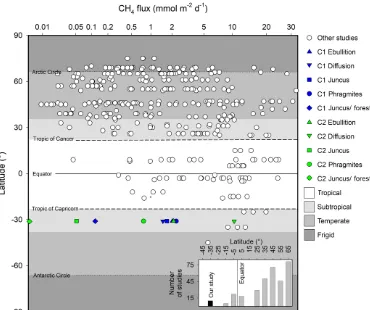
Figure 9.Summary of major CH₄wetland reviews by Bartlett and Harriss (1993) and Bastviken et al. (2011), as well as modelled fluxes by Cao et al. (1998) adapted from Jeffrey et al. (2019), highlighting latitudinal trends and bias from a variety of wetland systems. Inset figure highlights the number of studies in these reviews by latitudinal increments of 10◦poleward of the Equator. Note:xaxis scaled to highlight subtle differences between studies.

range of Northern Hemisphere subtropical systems of simi-lar latitudes (Fig. 9).

Although remediating degraded wetlands through re-flooding is a common technique to improve biodiversity, in-crease C sequestration, and improve downstream water qual-ity issues (Johnston et al., 2004, 2014), our results propose a nuanced dilemma for land use managers, as wetland re-mediation can potentially have net positive radiative forcing effects on the Earth’s climate due to high rates of CH4 pro-duction (Petrescu et al., 2015). This has also been shown to be particularly high during early remediation periods (Hemes et al., 2018). Our results suggest that seasonal wetlands emit less CH4on an areal basis than permanent wetlands, yet car-bon accumulation in these soils may be lower (Brown et al., 2019). Longer-term studies over annual cycles encompass-ing seasonal drivers and CH4 fluxes would further test this hypothesis of the different drivers between seasonal and per-manent wetland systems.

Our results also suggest that selective hydrological restora-tion of wetlands featuring sediments with abundant ther-modynamically favourable terminal electron acceptors (i.e. Fe(III) or SO2₄−) may be a (partial) biogeochemical solution

(also suggested by Hemes et al., 2018) to both remediate degraded sites whilst simultaneously mitigating some CH4 emissions. When Fe(III) and SO2₄−are abundant in anaero-bic environments they provide preferential terminal electron acceptors for microbial metabolism and thus limit methano-genesis via competitive exclusion (Achtnich et al., 1995). However, high rates of sulfate reduction coupled with Fe re-duction can also lead to the accumulation of metal sulfide minerals, e.g. pyrite and AVS (Johnston et al., 2014). Un-der permanently saturated and low oxygen conditions, metal sulfides will steadily accumulate and remain relatively be-nign. However, if the saturated state of remediated sites can-not be maintained, AVS may react with oxygen, resulting in the undesirable production of acidity and low pH conditions. Therefore, the remediation of wetlands for carbon storage should involve careful site selection to both limit CH4 pro-duction and to avoid redox-related geochemical by-products with detrimental environmental effects.

sul-emissions results were comparable to other wetlands of sim-ilar latitudes and contribute important data for both the un-derstudied Southern Hemisphere wetlands and seasonal sub-tropical wetland ecotypes.

Data availability. Data used for the composition of this paper can be obtained from https://data.mendeley.com/datasets/st4vyjc73f/ 1 (last access: 24 April 2019) (Jeffrey, 2019).

Author contributions. LCJ, DRT, SGJ, and DTM conceived the study. LCJ wrote the first draft. LCJ, DRT, SGJ, and KM conducted the fieldwork. LCJ, DRT, SGJ, DTM, ADLS, and KM reviewed and edited the paper.

Competing interests. The authors declare that they have no conflict of interest.

Acknowledgements. We would like to thank to Roz Hagan, Bob McDonnell, and Zach Ford for assistance in the field. We also thank Roz Hagan for processing the sediment cores, Isaac Santos and Ceylena Holloway for technical support, and the Mid-Coast Coun-cil for assistance. Luke C. Jeffrey acknowledges postgraduate sup-port from CSIRO. This work was supsup-ported by funding from the Australian Research Council (LP160100061). DRT and DTM ac-knowledge support from the Australian Research Council that par-tially funds their salaries (DE180100535 and DE150100581, re-spectively). Graphic components used in the conceptual model are courtesy of the Integration and Application Network, University of Maryland Centre for Environmental Science (http://ian.umces.edu/ symbols/, last access: June 2018).

Review statement. This paper was edited by Alexey V. Eliseev and reviewed by two anonymous referees.

References

Achtnich, C., Bak, F., and Conrad, R.: Competition for electron donors among nitrate reducers, ferric iron reducers, sulfate re-ducers, and methanogens in anoxic paddy soil, Biol. Fert. Soils, 19, 65–72, 1995.

121–128, 1990.

Armstrong, J. and Armstrong, W.: A convective through-flow of gases in Phragmites australis (Cav.) Trin. ex Steud, Aquat. Bot., 39, 75–88, 1991.

Armstrong, J., Jones, R., and Armstrong, W.: Rhizome phyllosphere oxygenation in Phragmites and other species in relation to redox potential, convective gas flow, submergence and aeration path-ways, New Phytol., 172, 719–731, 2006.

Bartlett, K. B. and Harriss, R. C.: Review and assessment of methane emissions from wetlands, Chemosphere, 26, 261–320, 1993.

Bastviken, D., Tranvik, L. J., Downing, J. A., Crill, P. M., and Enrich-Prast, A.: Freshwater methane emissions offset the conti-nental carbon sink, Science, 331, 50, 2011.

Bianchi, T. S.: Biogeochemistry of estuaries, Oxford University Press, New York, USA, 2007.

BOM: Taree Daily Weather Observations, available at: http://www. bom.gov.au/products/IDN60801/IDN60801.95784.shtml, last access: 12 April 2018.

Boman, A., Åström, M., and Fröjdö, S.: Sulfur dynamics in boreal acid sulfate soils rich in metastable iron sulfide – the role of arti-ficial drainage, Chem. Geol., 255, 68–77, 2008.

Boon, P. I., Mitchell, A., and Lee, K.: Effects of wetting and dry-ing on methane emissions from ephemeral floodplain wetlands in south-eastern Australia, Hydrobiologia, 357, 73–87, 1997. Bridgham, S. D., Moore, T. R., Richardson, C. J., and Roulet, N. T.:

Errors in greenhouse forcing and soil carbon sequestration esti-mates in freshwater wetlands: a comment on Mitsch et al. (2013), Landscape Ecol., 29, 1481–1485, 2014.

Brix, H., Sorrell, B. K., and Orr, P. T.: Internal pressurization and convective gas flow in some emergent freshwater macrophytes, Limnol. Oceanogr., 37, 1420–1433, 1992.

Brix, H., Sorrell, B. K., and Lorenzen, B.: Are Phragmites-dominated wetlands a net source or net sink of greenhouse gases?, Aquat. Bot., 69, 313–324, 2001.

Brown, D. R., Johnston, S. G., Santos, I. R., Holloway, C. J., and Sanders, C. J.: Significant organic carbon accumulation in two coastal acid sulfate soil wetlands, Geophys. Res. Lett., 46, 3245– 3251, https://doi.org/10.1029/2019gl082076, 2019.

Burdige, D.: Estuarine and coastal sediments–coupled biogeochem-ical cycling, Treatise on Estuarine and Coastal Science, 5, 279– 316, 2012.

Burton, E. D., Bush, R. T., and Sullivan, L. A.: Elemental sul-fur in drain sediments associated with acid sulfate soils, Appl. Geochem., 21, 1240–1247, 2006.

Burton, E. D., Bush, R. T., Sullivan, L. A., and Mitchell, D. R. G.: Reductive transformation of iron and sulfur in schwertmannite-rich accumulations associated with acidified coastal lowlands, Geochim. Cosmochim. Ac., 71, 4456–4473, https://doi.org/10.1016/j.gca.2007.07.007, 2007.

Cao, M., Gregson, K., and Marshall, S.: Global methane emission from wetlands and its sensitivity to climate change, Atmos. Env-iron., 32, 3293–3299, 1998.

Chanton, J. P., Arkebauer, T. J., Harden, H. S., and Verma, S. B.: Diel variation in lacunal CH4and CO2concentration andδ13C in Phragmites australis, Biogeochemistry, 59, 287–301, 2002. Claff, S. R., Sullivan, L. A., Burton, E. D., and Bush, R. T.: A

se-quential extraction procedure for acid sulfate soils: partitioning of iron, Geoderma, 155, 224–230, 2010.

Clevering, O. A. and Lissner, J.: Taxonomy, chromosome numbers, clonal diversity and population dynamics of Phragmites australis, Aquat. Bot., 64, 185–208, 1999.

Conrad, R.: Mechanisms controlling methane emission from wet-land rice fields, in: Biogeochemistry of Global Change, Springer, Boston, MA, USA, 317–335, 1993.

Costanza, R., de Groot, R., Sutton, P., van der Ploeg, S., Anderson, S. J., Kubiszewski, I., Farber, S., and Turner, R. K.: Changes in the global value of ecosystem services, Global Environ. Chang., 26, 152–158, 2014.

De La Cruz, A. A. and Hackney, C. T.: Enegry Value, Elemen-tal Composition, and Productivity of Belowground Biomass of a Juncus Tidal Marsh, Ecology, 58, 1165–1170, 1977.

Deverel, S. J., Ingrum, T., and Leighton, D.: Present-day oxidative subsidence of organic soils and mitigation in the Sacramento-San Joaquin Delta, California, USA, Hydrogeol. J., 24, 569–586, 2016.

Finlayson, C. M. and Rea, N.: Reasons for the loss and degradation of Australian wetlands, Wetl. Ecol. Manag., 7, 1–11, 1999. Freeman, C., Lock, M., and Reynolds, B.: Fluxes of CO₂, CH₄and

N2O from a Welsh peatland following simulation of water table draw-down: Potential feedback to climatic change, Biogeochem-istry, 19, 51–60, 1992.

GTCC: Cattai Wetlands Future Directions Strategy, avail-able at: https://www.midcoast.nsw.gov.au/files/assets/public/ document-resources/council/projects-documents/big-swamp/ cattai-wetlands-future-directions-strategy-adopted-may-14. pdf (last access: 10 March 2018), 2014.

Hemes, K. S., Chamberlain, S. D., Eichelmann, E., Knox, S. H., and Baldocchi, D. D.: A biogeochemical compromise: The high methane cost of sequestering carbon in restored wetlands, Geo-phys. Res. Lett., 45, 6081–6091, 2018.

Henneberg, A., Sorrell, B. K., and Brix, H.: Internal methane trans-port through Juncus effusus: experimental manipulation of mor-phological barriers to test above-and below-ground diffusion lim-itation, New Phytol., 196, 799–806, 2012.

Holmkvist, L., Ferdelman, T. G., and Jørgensen, B. B.: A cryptic sulfur cycle driven by iron in the methane zone of marine sed-iment (Aarhus Bay, Denmark), Geochim. Cosmochim. Ac., 75, 3581–3599, 2011.

Jeffrey, L.: Rhizosphere to the atmosphere: contrasting methane pathways, fluxes, and geochemical drivers across the terrestrial–

aquatic wetland boundary, Mendeley Data, v1, available at: https: //data.mendeley.com/datasets/st4vyjc73f/1, last access: 24 April 2019.

Jeffrey, L. C., Maher, D. T., Santos, I. R., McMahon, A., and Tait, D. R.: Groundwater, Acid and Carbon Dioxide Dynamics Along a Coastal Wetland, Lake and Estuary Continuum, Estuar. Coast., 39, 1325–1344, 2016.

Jeffrey, L. C., Maher, D. T., Johnston, S. G., Kelaher, B. P., Steven, A., and Tait, D. R.: Wetland methane emissions dominated by plant-mediated fluxes: Contrasting emissions pathways and sea-sons within a shallow freshwater subtropical wetland, Limnol. Oceanogr., https://doi.org/10.1002/lno.11158, 2019.

Johnston, S. G., Slavich, P. G., Sullivan, L. A., and Hirst, P.: Arti-ficial drainage of floodwaters from sulfidic backswamps: effects on deoxygenation in an Australian estuary, Mar. Freshwater Res., 54, 781–795, 2003.

Johnston, S. G., Slavich, P. G., and Hirst, P.: The effects of a weir on reducing acid flux from a drained coastal acid sulphate soil backswamp, Agr. Water Manage., 69, 43–67, 2004.

Johnston, S. G., Keene, A. F., Burton, E. D., Bush, R. T., and Sul-livan, L. A.: Quantifying alkalinity generating processes in a tidally remediating acidic wetland, Chem. Geol., 304, 106–116, 2012.

Johnston, S. G., Burton, E. D., Aaso, T., and Tuckerman, G.: Sul-fur, iron and carbon cycling following hydrological restoration of acidic freshwater wetlands, Chem. Geol., 371, 9–26, 2014. Karimian, N., Johnston, S. G., and Burton, E. D.: Acidity generation

accompanying iron and sulfur transformations during drought simulation of freshwater re-flooded acid sulfate soils, Geoderma, 285, 117–131, 2017.

Karimian, N., Johnston, S. G., and Burton, E. D.: Iron and sulfur cycling in acid sulfate soil wetlands under dynamic redox conditions: A review, Chemosphere, 197, 803–816, https://doi.org/10.1016/j.chemosphere.2018.01.096, 2018. Kim, J., Verma, S., Billesbach, D., and Clement, R.: Diel variation

in methane emission from a midlatitude prairie wetland: signifi-cance of convective throughflow in Phragmites australis, Jo. Geo-phys. Res.-Atmos., 103, 28029–28039, 1998.

Kirschke, S., Bousquet, P., Ciais, P., Saunois, M., Canadell, J. G., Dlugokencky, E. J., Bergamaschi, P., Bergmann, D., Blake, D. R., Bruhwiler, L., Cameron-Smith, P., Castaldi, S., Chevallier, F., Feng, L., Fraser, A., Heimann, M., Hodson, E. L., Houwel-ing, S., Josse, B., Fraser, P. J., Krummel, P. B., Lamarque, J.-F., Langenfelds, R. L., Le Quéré, C., Naik, V., O’Doherty, S., Palmer, P. I., Pison, I., Plummer, D., Poulter, B., Prinn, R. G., Rigby, M., Ringeval, B., Santini, M., Schmidt, M., Shindell, D. T., Simpson, I. J., Spahni, R., Steele, L. P., Strode, S. A., Sudo, K., Szopa, S., van der Werf, G. R., Voulgarakis, A., van Weele, M., Weiss, R. F., Williams, J. E., and Zeng, G.: Three decades of global methane sources and sinks, Nat. Geosci., 6, 813–823, https://doi.org/10.1038/ngeo1955, 2013.

Knorr, K.-H., Glaser, B., and Blodau, C.: Fluxes and 13C iso-topic composition of dissolved carbon and pathways of methano-genesis in a fen soil exposed to experimental drought, Bio-geosciences, 5, 1457–1473, https://doi.org/10.5194/bg-5-1457-2008, 2008.

788, https://doi.org/10.5194/bg-10-753-2013, 2013.

Milberg, P., Tornqvist, L., Westerberg, L. M., and Bastviken, D.: Temporal variations in methane emissions from emergent aquatic macrophytes in two boreonemoral lakes, AoB Plants, 9, plx029, https://doi.org/10.1093/aobpla/plx029, 2017.

Mitsch, W. J., Bernal, B., Nahlik, A. M., Mander, Ü., Zhang, L., Anderson, C. J., Jørgensen, S. E., and Brix, H.: Wetlands, carbon, and climate change, Landscape Ecol., 28, 583–597, 2013. Moore, G. E., Burdick, D. M., Peter, C. R., and Keirstead, D. R.:

Be-lowground biomass of Phragmites australis in coastal marshes, Northeast. Nat., 19, 611–627, 2012.

Mulvey, P.: Pollution, prevention and management of sulphidic clays and sands, Proceedings National Conference on Acid Sul-phate Soils, edited by: Bush, R., 116–129, 1993.

Nedwell, D. B. and Watson, A.: CH4 production, oxidation and emission in a UK ombrotrophic peat bog: influence of SO2₄− from acid rain, Soil Biol. Biochem., 27, 893–903, 1995. Neubauer, S. C. and Megonigal, J. P.: Moving beyond global

warming potentials to quantify the climatic role of ecosystems, Ecosystems, 18, 1000–1013, 2015.

Page, K. and Dalal, R.: Contribution of natural and drained wetland systems to carbon stocks, CO2, N2O, and CH4fluxes: an Aus-tralian perspective, Soil Res., 49, 377–388, 2011.

Pangala, S. R., Enrich-Prast, A., Basso, L. S., Peixoto, R. B., Bastviken, D., Hornibrook, E. R., Gatti, L. V., Marotta, H., Calazans, L. S. B., and Sakuragui, C. M.: Large emissions from floodplain trees close the Amazon methane budget, Nature, 552, 230, 2017.

Penhale, P. A. and Wetzel, R. G.: Structural and functional adapta-tions of eelgrass (Zostera marina L.) to the anaerobic sediment environment, Can. J. Bot., 61, 1421–1428, 1983.

Pereyra, A. S. and Mitsch, W. J.: Methane emissions from freshwa-ter cypress (Taxodium distichum) swamp soils with natural and impacted hydroperiods in Southwest Florida, Ecol. Eng., 114, 46–56, 2018.

Petrescu, A. M., Lohila, A., Tuovinen, J. P., Baldocchi, D. D., De-sai, A. R., Roulet, N. T., Vesala, T., Dolman, A. J., Oechel, W. C., Marcolla, B., Friborg, T., Rinne, J., Matthes, J. H., Merbold, L., Meijide, A., Kiely, G., Sottocornola, M., Sachs, T., Zona, D., Varlagin, A., Lai, D. Y., Veenendaal, E., Parmentier, F. J., Skiba, U., Lund, M., Hensen, A., van Huissteden, J., Flanagan, L. B., Shurpali, N. J., Grunwald, T., Humphreys, E. R., Jackowicz-Korczynski, M., Aurela, M. A., Laurila, T., Gruning, C., Corradi, C. A., Schrier-Uijl, A. P., Christensen, T. R., Tamstorf, M. P., Mastepanov, M., Martikainen, P. J., Verma, S. B., Bernhofer, C., and Cescatti, A.: The uncertain climate footprint of wetlands

un-mochim. Ac., 60, 3169–3175, 1996.

Rayment, G. and Higginson, F. R.: Australian laboratory handbook of soil and water chemical methods, Inkata Press Pty Ltd, Mel-bourne, Australia, 1992.

Sammut, J., White, I., and Melville, M.: Acidification of an estuar-ine tributary in eastern Australia due to drainage of acid sulfate soils, Mar. Freshwater Res., 47, 669–684, 1996.

Saunois, M., Bousquet, P., Poulter, B., Peregon, A., Ciais, P., Canadell, J. G., Dlugokencky, E. J., Etiope, G., Bastviken, D., Houweling, S., Janssens-Maenhout, G., Tubiello, F. N., Castaldi, S., Jackson, R. B., Alexe, M., Arora, V. K., Beerling, D. J., Berga-maschi, P., Blake, D. R., Brailsford, G., Brovkin, V., Bruhwiler, L., Crevoisier, C., Crill, P., Covey, K., Curry, C., Frankenberg, C., Gedney, N., Höglund-Isaksson, L., Ishizawa, M., Ito, A., Joos, F., Kim, H.-S., Kleinen, T., Krummel, P., Lamarque, J.-F., Langen-felds, R., Locatelli, R., Machida, T., Maksyutov, S., McDonald, K. C., Marshall, J., Melton, J. R., Morino, I., Naik, V., O’Doherty, S., Parmentier, F.-J. W., Patra, P. K., Peng, C., Peng, S., Peters, G. P., Pison, I., Prigent, C., Prinn, R., Ramonet, M., Riley, W. J., Saito, M., Santini, M., Schroeder, R., Simpson, I. J., Spahni, R., Steele, P., Takizawa, A., Thornton, B. F., Tian, H., Tohjima, Y., Viovy, N., Voulgarakis, A., van Weele, M., van der Werf, G. R., Weiss, R., Wiedinmyer, C., Wilton, D. J., Wiltshire, A., Wor-thy, D., Wunch, D., Xu, X., Yoshida, Y., Zhang, B., Zhang, Z., and Zhu, Q.: The global methane budget 2000–2012, Earth Syst. Sci. Data, 8, 697–751, https://doi.org/10.5194/essd-8-697-2016, 2016.

Sivan, O., Antler, G., Turchyn, A. V., Marlow, J. J., and Orphan, V. J.: Iron oxides stimulate sulfate-driven anaerobic methane ox-idation in seeps, P. Natl. Acad. Sci. USA, 111, E4139–E4147, 2014.

Sorrell, B. K. and Boon, P. I.: Convective gas flow in Eleocharis sphacelata R. Br.: methane transport and release from wetlands, Aquat. Bot., 47, 197–212, 1994.

Stocker, T. F., Qin, D., Plattner, G.-K., Tignor, M., Allen, S. K., Boschung, J., and Midgley, P. M.: Climate Change 2013: The Physical Science Basis. Contribution of Working Group I to the Fifth Assessment Report of the Intergovernmental Panel on Cli-mate Change, 1535 pp., in: Cambridge Univ. Press, Cambridge, UK, and New York, USA, 2013.

Tucker, G. C.: The genera of Arundinoideae (Gramineae) in the southeastern United States, J. Arnold Arboretum, 71, 145–177, 1990.

Villa, J. A. and Bernal, B.: Carbon sequestration in wetlands, from science to practice: An overview of the biogeochemical process, measurement methods, and policy framework, Ecol. Eng., 114, 115–128, https://doi.org/10.1016/j.ecoleng.2017.06.037, 2018. Walker, P. H.: Seasonal and stratigraphic controls in coastal

flood-plain soils, Soil Res., 10, 127–142, 1972.

Wang, Z., Zeng, D., and Patrick, W. H.: Methane emissions from natural wetlands, Environ. Monit. Assess., 42, 143–161, 1996. White, I., Melville, M., Wilson, B., and Sammut, J.: Reducing

acidic discharges from coastal wetlands in eastern Australia, Wetl. Ecol. Manag., 5, 55–72, 1997.

Whiting, G. J. and Chanton, J. P.: Plant-dependent CH4emission in a subarctic Canadian fen, Global Biogeochem. Cy., 6, 225–231, 1992.

Whiting, G. J. and Chanton, J. P.: Greenhouse carbon balance of wetlands: methane emission versus carbon sequestration, Tellus B, 53, 521–528, 2001.