Towards Thermal Aware Workload Scheduling in a Data Center

Towards Thermal Aware Workload Scheduling in a

Data Center

Lizhe Wang

, Gregor von Laszewski

, Jai Dayal

, Xi He

, Andrew J. Younge

and Thomas R. Furlani

†

Service Oriented Cyberinfrastructure Lab

Rochester Institute of Technology

Rochester, NY 14623

‡

Center for Computational Research

State University of New York at Buffalo

Buffalo, NY 14203

Abstract—High density blade servers are a popular technology for data centers, however, the heat dissipation density of data cen-ters increases exponentially. There is strong evidence to support that high temperatures of such data centers will lead to higher hardware failure rates and thus an increase in maintenance costs. Improperly designed or operated data centers may either suffer from overheated servers and potential system failures, or from overcooled systems, causing extraneous utilities cost. Minimizing the cost of operation (utilities, maintenance, device upgrade and replacement) of data centers is one of the key issues involved with both optimizing computing resources and maximizing business outcome.

This paper proposes an analytical model, which describes data center resources with heat transfer properties and workloads with thermal features. Then a thermal aware task scheduling algorithm is presented which aims to reduce power consumption and temperatures in a data center. A simulation study is carried out to evaluate the performance of the algorithm. Simulation results show that our algorithm can significantly reduce tem-peratures in data centers by introducing endurable decline in performance.

Keywords - Thermal aware, data center, task scheduling

I. INTRODUCTION

Recently electricity usage has become a major IT concern for data center computing. In fact, the electricity costs for running and cooling computers generally are considered to be the bulk of the IT budget. As reported by U.S. Environmental Protection Agency (EPA), 61 billion kilowatt-hours of power was consumed in data centers in 2006, which is 1.5% of all US electricity consumption and worthy of $4.5 billion [1]. In fact, the energy consumption in data centers doubled between 2000 and 2006. Furthermore, the EPA estimates that the energy usage will double again by 2011.

A large scale data center’s annual energy cost can be several millions of US dollars. In fact, it is reported that cooling costs can be up to 50% of the total energy cost [2]. Even with more efficient cooling technologies in IBM’s BlueGene/L and TACC’s Ranger, cooling cost still remains a significant portion of the total energy cost for these data centers. It is also noted that the life of a computer system is directly related to its operating temperature. Based on Arrhenius time-to-fail

model [3], every 10◦C increase of temperature leads to a

doubling of the system failure rate. Hence, it is recommended

that computer components be kept as cool as possible for maximum reliability, longevity, and return on investment [4]. Therefore, thermal aware resource management for data centers has recently attracted much research interest from high performance computing communities. The most elaborate thermal aware schedule algorithms for tasks in data centers are with computational fluid dynamics (CFD) models [5], [6]. Some research [7], [8] declares that the CFD based model is too complex and is not suitable for online scheduling. This has lead to the development of some less complex online scheduling algorithms. Sensor-based fast thermal evaluation model [9], [10], Generic Algorithm & Quadratic Programming [7], [11], and the Weatherman – an automated online predictive thermal mapping [12] are a few examples.

Our work differs from the above systems in that we’ve de-veloped some elaborate heat transfer models for data centers. Our model is a trade-off between the complex CFD model and the other on-line scheduling algorithms. Our model, therefore, is less complex than the CFD models and can be used for on-line scheduling in data centers. It can provide more accurate description of data center thermal maps than [7], [11]. In detail, we study a temperature–based workload model and a thermal-based data center model. This paper then defines the thermal aware workload scheduling problem for data centers and presents a thermal-aware scheduling algorithm for data center workloads. We use simulations to evaluate thermal-aware workload scheduling algorithms and discuss the trade-off between throughput, cooling cost other performance met-rics. Our unique contribution is shown as follows. We propose a general framework for thermal aware resource management for data centers. Our framework is not bound to any specific model, such as the RC-thermal model, the CFD model, or a task-termparature profile. A new heuristic for thermal aware workload scheduling is developed and evaluated, in terms of performance loss, cooling cost and reliability.

2

Section VI.

II. RELATED WORK AND BACKGROUND

A. Data center operation

The racks in a typical data center with a standard cooling layout based on under-floor cold air distribution are back-to-back and laid out in rows on a raised floor over a shared plenum. Modular computer room air conditioning (CRAC) units along the walls circulate warm air from the machine room over cooling coils, and direct the cooled air into the shared plenum. As shown in Figure 2, the cooled air enters the machine room through floor vent tiles in alternating aisles between the rows of racks. Aisles containing vent tiles are cool aisles; equipment in the racks is oriented so their intake draws inlet air from cool aisles. Aisles without vent tiles are hot aisles, providing access to the exhaust air and, typically, rear panels of the equipment [13].

Thermal imbalances interfere with efficient cooling opera-tion. Hot spots create a risk of redlining servers by exceeding the specified maximum inlet air temperature, damaging elec-tronic components and causing them to fail prematurely. Non-uniform equipment loads in the data center cause some areas to heat more than others, while irregular air flows cause some areas to cool less than others. The mixing of hot and cold air in high heat density data centers leads to complex airflow patterns that create hot spots. Therefore, objectives of thermal aware workload scheduling are to reduce both the maximum temperature for all compute nodes and the imbalance of the thermal distribution in a data center. In a data center, the thermal distribution and computer node temperatures can be obtained by deploying ambient temperature sensors, on-board sensors [9], [10], and with software management architectures like Data Center Observatory [14], Mercury & Freon [15], LiquidN2 & C-Oracle[16].

B. Task-temperature profiling

Given certain compute processor and steady ambient tem-perature, a task-temperature profile is the temperature increase along with the task execution. It has been observed that differ-ent types of computing tasks generate differdiffer-ent amount of heat, therefore featuring with distinct task-temperature profiles [17]. Task-temperature profiles can be obtained by using some profiling tools. Figure 1 shows a task-temperature profile, which is obtained by running SPEC 2000 benchmark (crafty) on a IBM BladeCenter with 2 GB memory and Red Hat Enterprise Linux AS 3 [17].

It is constructive and reasonably realistic to assume that the knowledge of task-temperature profile is available based on the discussion [18], [19] that task-temperature can be well approximated using appropriate prediction tools and methods.

III. SYSTEM MODELS AND PROBLEM DEFINITION

A. Compute resource model

This section presents formal models of data centers and workloads, and a thermal aware scheduling algorithm, which allocate compute resources in a data center for incoming

0 20 40 60 80 100 120 140 160 180

0 5 10 15 20 25 crafty

Increase in core temperature (C)

Time (s)

0 10 20 30 40 50 60 70

0 5 10 15 20 25 gzip

Increase in core temperature (C)

Time (s)

(a)

(b)

0 50 100 150 200 250 300 350 400

0 5 10 15 20 25 mcf

Increase in core temperature (C)

Time (s)

0 100 200 300 400 500 600

0 5 10 15 20 25 swim

Increase in core temperature (C)

Time (s)

(c)

(d)

0 20 40 60 80 100 120 140 160 180 200

0 5 10 15 20 25 vortex

Increase in core temperature (C)

Time (s)

0 20 40 60 80 100 120 140 160 180

0 5 10 15 20 25 wupwise

Increase in core temperature (C)

Time (s)

(e)

(f)

Fig. 1.

Task temperature profiles for the SPEC’2K benchmarks (a)

crafty

, (b)

gzip

, (c)

mcf

, (d)

swim

, (e)

vortex

, and (f)

wupwise

.

Fig. 1. Task-temperature profile of SPEC2000 (crafty) [17]

workloads with the objective of reducing temperature in the data center.

A data centerDataCenteris modeled as:

DataCenter={N ode, T herM ap} (1)

where,

N odeis a set of compute nodes,

T herM apis the thermal map of a data center.

A thermal map of a data center describes the ambient temperature field in a 3-dimensional space. The temperature field in a data center can be defined as follows:

T herM ap=T emp(< x, y, z >, t) (2)

It means that the ambient temperature in a data center is a

variable with its space location (x, y, z)and timet. Figure 2

shows a thermal map [20] example in a data center.

4 DELL.COM/PowerSolutions Reprinted from Dell Power Solutions, February 2008. Copyright © 2008 Dell Inc. All rights reserved.

heat load for this example data center is 129 kW. The total rack airflow demand is 20,000 cfm, and the computer room air-conditioning units supply 22,600 cfm of cooling air at a temperature of 55°F. The maximum acceptable inlet air temperature is 75°F. Figure 2 shows the calculated air-flow distribution through the perforated tiles, which have flow rates ranging from 325 cfm to 640 cfm. Because all the per-forated tiles have the same open area, this variation indicates a nonuniform pressure distribution under the raised floor, as shown in Figure 3.

The number of overheated racks— those with an inlet air temperature greater than 75°F—can serve to quantify cooling performance in the data center. Figure 4 shows the temperature distribution at the front of the racks, with the 13 overheated racks marked by red warning lights. These results indicate that although the total cooling airflow is sufficient, the airflow distribution is not, because the amount of cooling air available in front of certain racks does not meet the airflow demand. Consequently, the servers in the top sec-tion of these racks draw hotter air (origi-nating at the back of the racks) than those at the bottom (see Figure 5).

Choosing an optimal configuration

Several factors contribute to the poor cooling performance of the example layout—for example, in addition to the hot exhaust carried between rows, many racks lack perforated tiles in front of them. Figure 6 shows a modified layout that adheres to a hot aisle/cold aisle pattern,

Figure 3. Airflow pattern and pressure distribution under the raised floor in the example data center

Figure 4. Rack inlet temperatures and overheated racks in the example data center In addition to pursuing an overall strategy of energy efficiency at the enterprise

level, IT staff can follow specific best practices when designing or optimizing a data center that can help reduce power consumption and create efficient cooling:

Use blanking panels in open rack space Ê

!

Seal cable panel cutout spaces Ê

!

Employ hot aisle/cold aisle layouts Ê

!

Limit the number of perforated tiles Ê

!

Use no perforated tiles in hot aisles Ê

!

Monitor under-floor static pressure at multiple points Ê

!

Check airflow balance regularly Ê

!

Use computational fluid dynamics modeling to engineer airflow Ê

!

Raise computer room temperatures Ê

!

Avoid mixing supply and exhaust air Ê

!

FOLLOWING COOLING BEST PRACTICES FOR DATA CENTER DESIGN

Fig. 2. A thermal map of a typical data center [20]

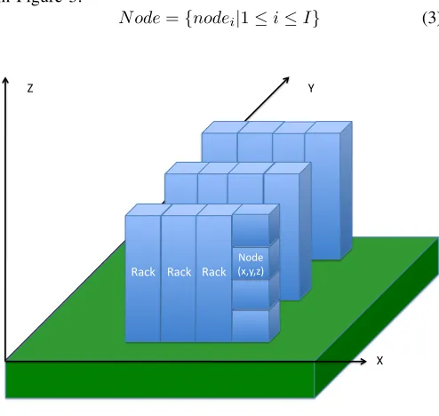
We consider a homogeneous computer center: all compute nodes have identical hardware and software configurations.

3

in Figure 3:

N ode={nodei|1≤i≤I} (3)

!" #"

$" %&'("

)*+"&,-" )*+"&,-"

%&'(" %&'(" 1234356".*/0"

Fig. 3. Layout of a data center

The ith_{compute node is described as follows:}

nodei= (< x, y, z >, ta, T emp(t)) (4)

< x, y, z > isnodei’s location in a 3-dimensional space.

ta _{is the time whennode}

i is available for job execution.

T emp(t)is the temperature ofnodei,t is time.

The process of heat transfer of nodei is described with a

RC-thermal model [21], [22], [23]. As shown in Figure 4,P

denotes the power consumption of compute node at current

timet,C is the thermal capacitance of the compute node, R

denotes the thermal resistance, and T emp(nodei. < x, y, z >

, t)represents the ambient temperature ofnodeiin the thermal

map. Therefore the heat transfer between a compute node and its ambient environment is described in the following equation (also shown in Figure 5):

nodei.T emp(t) =RC×

dnodei.T emp(t)

dt

+T emp(nodei. < x, y, z >, t)−RP (5)

!" #" $" %&'()*+(,-./0"

+(,-.%&'()*12343563/0"

Fig. 4. RC-thermal model

It is supposed that an initial die temperature of a compute

node at time 0 is nodei.T emp(0), P and T emp(nodei. <

x, y, z >, t)are constant during the period [0, t] (this can be true when calculating a short period). Then the compute node

temperature N odei.T emp(t)is calculated as follows:

nodei.T emp(t) =P R+T emp(nodei. < x, y, z >,0)+

(nodei.T emp(0)−P R−T emp(nodei. < x, y, z >,0))×e−

t RC

(6)

B. Workload model

Workloads in a data center are modeled as a set of jobs,

J ob={jobj|1≤j≤J} (7)

J is the total number of incoming jobs. jobj is an incoming

job, which is described as follows:

jobj= (p, tarrive, tstart, treq,∆T emp(t)) (8)

where,

pis the required compute node number ofjobj,

tarrive is the arrival time ofjobj, tstart is the starting time of jobj,

treq is the required execution time ofjobj,

∆T emp(t)is the task-temperature profile ofjobj on compute nodes of a data center.

C. Online task temperature calculation

When a job jobj runs on certain compute node nodei,

the job execution will increase the node’s temperature jobj.∆T emp(t). In the mean time, the node also disseminates heat to ambient environment, which is calculated by Equation

(6). Therefore the online node temperature ofnodei is

calcu-lated as follows:

nodei.T emp(t) =nodei.T emp(0)+jobj.∆T emp(t)−

{P R+T emp(nodei. < x, y, z >,0)+

(nodei.T emp(0)−P R−T emp(nodei. < x, y, z >,0))×e−

t

RC}

(9)

!" #$%!&'()*+"),-'+"" !*./%!')0'(*!1('"0(,2+'"

34+54'"!*./%!')0'(*!1('" 6,-'578')09!:"

8')096,-'57;<=>=?@=!:"

A#B"

6,-'578')09C:"

D. Research issue definition

Based on discussion on above, a job schedule is a map

from a jobjobj to certain work nodenodeiwith starting time

jobj.start:

schedulej:jobj→(nodei, jobj.tstart) (10)

A workload schedule Schedule is a set of job schedules

{schedulej|jobj ∈J ob} for all jobs in the workload:

Schedule={schedulej|jobj∈J ob} (11)

We define the workload starting time T0 and finished time

T∞ as follows:

T∞= max

1≤j≤J{jobj.t

start_+job

j.treq} (12)

T0= min

1≤j≤J{jobj.t arrive

} (13)

Then the workload response timeTresponse is calculated as

follows:

Tresponse=T∞−T0 (14)

Assuming that the specified maximum inlet air temperature

in a data center is T EM Pmax, thermal aware workload

scheduling in a data center could be defined as follows: given

a workload set J ob and a data center DataCenter, find

an optimal workload schedule, Schedule, which minimizes

Tresponse of the workload J ob:

minTresponse (15)

subject to:

max

1≤i≤I{nodei.T emp(t)|T0≤t≤T∞} ≤T empmax (16)

E. Discussion

This subsection proves that the research issue defined above is an NP-hard problem. If a compute node’s temperature is higher than the specified maximum temperature, the compute node should cool down with no task execution. To be

consis-tent, we can say that there is a dummy taskj0running on this

node during the period of cooling down.

Without lost of generosity, we can setT0= 0, which means

that tasks are scheduled from the time of 0. Then Equation 15 can be expressed as follows:

minTresponse (17)

Tresponse= max 1≤i≤I{

X

jobj∈J obi

{jobj.treq×xj}} (18)

where

xj =

0 ifj= 0 1 ifj >0

J obi={jobj|jobj is executed onnodei}

Let T IM Ebe a constant,

jobj.tsave=T IM E−jobj.treq (19)

Then the research issue for thermal aware scheduling can

be expressed as:

maxTsave (20)

Tsave= min 1≤i≤I{

X

jobj∈J obi

{(jobj.tsave)×xj}} (21)

where,

xj=

0 if j= 0 1 if j >0

J obi={jobj|jobj is executed on nodei}

subject to:

max

1≤i≤I{nodei.T emp(t)|T0≤t≤T∞} ≤T empmax (22) The above expression is equivalent to the well know multiple-choice knapsack problem (MCKP), which has been proven to be an NP-hard problem [24]. Therefore, the thermal aware scheduling issue defined in subsection III-D is an NP-hard problem.

IV. THERMAL AWARE WORKLOAD SCHEDULING

ALGORITHM

This section discusses our Thermal Aware Scheduling Algo-rithm (TASA). The key idea of TASA is to schedule ”hot” jobs on ”cold” compute nodes and tries to reduce the temperatures of compute nodes.

Based on

• temperatures of ambient environment and compute nodes

which can be obtained from temperature sensors,

• on-line job-temperature profiles

the compute node temperature after job execution can be predicated with Eq. E:online. TASA algorithm schedules jobs based on the temperature prediction.

Algorithm 1 presents a Thermal Aware Scheduling Algo-rithm (TASA). Lines 1– 4 initialize variables. Line 1 sets the initial time stamp to 0. Lines 2 – 4 set compute nodes available time to 0, which means all nodes are available from the beginning.

Lines 5 – 29, of Algorithm 1 schedule jobs periodically

with an interval of Tinterval Lines 5 and 6 update thermal

map T herM ap and current temperatures of all nodes from the input ambient sensors and on-board sensors. Then, line 7 sorts all jobs with decreased jobj.∆T emp(jobj.treq): jobs are sorted from “hottest” to “coolest”. Line 8 sorts all nodes with increasing node temperature at the next available time, nodei.T emp(nodei.ta): nodes are sorted from “coolest” to “hottest” when nodes are available.

Lines 9-14 cool down the over-heated compute nodes. If a node’s temperature is higher than a pre-defined temperature T EM Pmax_{, then the node is cooled for a period of T}cool_.

During the period of Tcool_{, there is no job scheduled on this}

node. This node is then inserted into the sorted node list, which keeps the increased node temperature at next available time.

5

Algorithm 1 Thermal Aware Scheduling Algorithm (TASA)

01 t=0

02 Fori= 1 TOI DO

03 nodei.ta=0;

04 ENDFOR

05 update thermal mapT herM ap

06 updatenodei.T emp(t),nodei∈N ode

07 sort J ob with decreasedjobj.∆T emp(jobj.treq)

08 sort N odewith increasednodei.T emp(nodei.ta)

09 FOR nodei∈N odeDO

10 IF (nodei.T emp(nodei.ta)≥T EM Pmax) TEHN

11 nodei.ta=nodei.ta+Tcool

12 calculatenodei.T emp(nodei.ta) with Eq. 6

13 insertnodei intoN ode, keep the increased order

of nodei.T emp(nodei.ta)inN ode

14 ENDIF

15 ENDFOR

16 FOR j= 1TOJ DO

17 get jobj.pnodes from sortedN odelist,

which are{nodej1, nodej2, . . . , nodejp} 18 t0= max{nodek.ta}

nodek∈ {nodej1, nodej2, . . . , nodejp} 19 FOR nodek ∈ {nodej1, nodej2, . . . , nodejp}

20 nodek.ta=t0+jobj.treq

21 ENDFOR

22 schedule jobj on{nodej1, nodej2, . . . , nodejp}

23 jobj.tstart=t0

24 calculate nodek.T emp(nodek.ta)with Eq. 6 & 9

nodek∈ {nodej1, nodej2, . . . , nodejp}

25 insert {nodej1, nodej2, . . . , nodejp} intoN ode

keep the increased order ofnodei.T emp(nodei.ta)

nodei∈N ode

26 ENDFOR

27 t=t+Tinterval

28 Accept incoming jobs

29 go to 05

from sorted job list, which is the “hottest” job and line 17 allocates the job with a number of required nodes , which are the “coolest”. Lines 18 – 20 find the earliest starting time of the job on these nodes. After that, line 24 calculates the temperature of next available time for these nodes. Then these nodes are inserted into the sorted node list, which keeps the increased node temperature at next available time.

Algorithm 1 waits a for period of Tinterval and accepts

incoming jobs. It then proceeds to the next scheduling round.

V. SIMULATION ANDPERFORMANCE EVALUATION

A. Simulation environment

We simulate a real data center environment based on the Center for Computational Research (CCR) of State University of New York at Buffalo. All jobs submitted to CCR are logged during a 30-day period, from 20 Feb. 2009 to 22 Mar. 2009. CCR’s resources and job logs are used as input for our simulation of the Thermal Aware Scheduling Algorithm (TASA).

CCR’s computing facilities include a Dell x86 64 Linux Cluster consisting of 1056 Dell PowerEdge SC1425 nodes, each of which has two Irwindale processors (2MB of L2 cache, either 3.0GHz or 3.2GHz) and varying amounts of main memory. The peak performance of this cluster is over 13TFlop/s.

The CCR cluster has a single job queue for incoming jobs. All jobs are scheduled with a First Come First Serve (FCFS) policy. There were 22385 jobs submitted to CCR during the period from 20 Feb. 2009 to 22 Mar. 2009. Figure 6, Figure 7 and Figure 8 show the distribution of job execution time, job size (required processor number) and job arrival rate in the log. We can see that 79% jobs are executed on one processor and job execution time ranges from several minutes to several hours.

In the simulation, we take the all 22385 jobs in the log as input for the workload module of TASA. We also measure the temperatures of all computer nodes and ambient environment with off-board sensors. Therefore the thermal map of data centers and job-temperature profiles are available. Online temperatures of all computer nodes can also be accessed from CCR web portal.

In the following section, we simulate the Thermal Aware Scheduling Algorithm (TASA) based on the job-temperature profile, job information, thermal maps, and resource informa-tion obtained in CCR log files. We evaluate the thermal aware scheduling algorithm by comparing it with the original job execution information logged in the CCR, which is scheduled by FCFS. In the simulation of TASA, we set the maximum

temperature threshold to 125◦F.

B. Experiment results and discussion

1) Data center temperature: Firstly we consider the

max-imum temperature in a data center as it correlates with the

cooling system operating level. We use∇T empmax _{to show}

the maximum temperature reduced by TASA.

∇T empmax=T empmax_{f cf s}−T empmax_tasa (23)

where, T empmax

f cf sis the maximum temperature in a data center where FCFS is employed, and

T empmax

tasa is the maximum temperature in a data center where

TASA is employed.

In the simulation we got∇T empmax_{= 6.1} ◦_{F. Therefore,}

TASA reduces 6.1 ◦F of the maximum temperature in CCR.

It is reported that every1◦F reduced in a data center, 2%

8% 7%

8%

19%

2%

3% _6% 6% 2%

3% 16% 19% 2%

<5mins 5~10mins 10~15mins 15~20mins 20~30mins 30~60mins 60~90mins 90~120mins 2~4hours 4~6hours 6~8hours 8~50 >50hours

Fig. 6. Job execution time distribution

79%

< 1% 4% 8% 2% 4% 2%

1 processor 2 processors 4 processors 6~10 processors 11~20 processors 21!50 processors > 50 processors

Fig. 7. Job size distribution

Jobs arrival rate

Time(Hour)

Jobs # arr

iv

ed hour

ly

0 200 400 600

0

500

1000

1500

2000

2500

Fig. 8. Job arrive rate distribution

of the cooling system in CCR, which is up to 6% of total power consumption of CCR. It is estimated that total power consumption of CCR is around 80000 KW/Hour. Thus the TASA can save around 5000 KW/Hour power consumption.

We also consider the average temperatures in a data center, which relates the system reliability. In Figure 11 the red line shows the average ambient temperatures of all compute nodes, which is scheduled by TASA and blue line shows the average temperatures of all nodes in the log files , which were scheduled by FCFS. Compared with FCFS, the average

temperature reduced by TASA is 16◦F.

2) Job response time: We have reduced power consumption

and have increase the system reliability, both by decreasing the data center temperatures. However, we must consider that there may be trade offs by an increased response time.

The response time of a jobjobj.tres is defined as job

exe-cution time (jobj.treq) plus job queueing time(jobj.tstart−

jobj.tarrive), as shown below:

jobj.tres=jobj.treq+jobj.tstart−jobj.tarrive (24)

To evaluate the algorithm from the view point of users, job response time indicates how long it takes for job results to return to the users.

As the thermal aware scheduling algorithm intends to delay scheduling jobs to some over-hot compute nodes, it may increase the job response time. Figure 9 shows the response time of FCFS and Figure 10 shows the response time of TASA. In the simulation we calculate the overall job response time overhead as follows:

overhead= X

1≤j≤J

jobj.trestasa−jobj.tresf cf s

jobj.tresf cf s

(25)

In the simulation, we got the overhead = 13.9%. Which

means that we reduce the 6.1◦F of temperature in CCR data

center by paying cost of increasing 13.9% job response time.

VI. CONCLUSION AND FUTURE WORK

With the advent of Cloud computing, data centers are becoming more important in modern cyberinfrastructures for high performance computing. However current data centers

Fig. 9. Job response time of FCFS

Fig. 10. Job response time of TASA

7

!"# $"# %"# &""# &&"#

&# '&# &"&# &'&# ("&# ('&# )"&# )'&# *"&# *'&# '"&# ''&# +"&# +'&# !"&#

!"

#$

%&

#'(

#)*#$

%(+#',-.'

/0)#',12+$.'

,-,.# /0.0#

Fig. 11. Average temperature of all compute nodes

factors such as resource power supply, cooling system supply, and other maintenance. This produces CO2 emissions and signicantly contributes to the growing environmental issue of Global Warming. Green computing, a new trend for high-end computing, attempts to alleviate this problem by delivering both high performance and reduced power consumption, ef-fectively maximizing total system efciency.

Currently power supply for cooling systems can occupy up to 40%-50% of total power consumption in a data center. This paper presents a thermal aware scheduling algorithm for data centers to reduce the temperatures in data center. Specifically, we present the design and implementation of an efcient scheduling algorithm to allocate workloads based on their task-termpatrue profiles and find suitable resources for their execution. The algorithm is studied through a simulation based on real operation information in CCR data center. Test results and performance discussion justify the design and implementation of the thermal aware scheduling algorithm.

In the future work, we are interested to discuss the tradeoff between temperature reduced and the response time increased. As backfilling algorithm is popular in parallel systems, we plan to integrate the backfilling algorithm into the TASA to improve the system performance.

REFERENCES

[1] “Report to Congress on Server and Data Center Energy Efficiency.” [Online]. Available: http://www.energystar.gov/ia/partners/prod development/downloads/EPA Datacenter Report Congress Final1.pdf [2] R. Sawyer, “Calculating Total Power Requirements for Data Centers,”

American Power Conversion, Tech. Rep., 2004.

[3] P. W. Hale, “Acceleration and time to fail,” Quality and Reliability Engineering International, vol. 2, no. 4, pp. 259–262, 1986.

[4] “Operating Temperature vs System Reliability,” Website, 2009. [Online]. Available: http://www.pcpower.com/technology/optemps/

[5] J. Choi, Y. Kim, A. Sivasubramaniam, J. Srebric, Q. Wang, and J. Lee, “A CFD-Based Tool for Studying Temperature in Rack-Mounted Servers,”IEEE Trans. Comput., vol. 57, no. 8, pp. 1129–1142, 2008. [6] A. H. Beitelmal and C. D. Patel, “Thermo-Fluids Provisioning of a

High Performance High Density Data Center,”Distributed and Parallel Databases, vol. 21, no. 2-3, pp. 227–238, 2007.

[7] Q. Tang, S. K. S. Gupta, and G. Varsamopoulos, “Energy-Efficient Thermal-Aware Task Scheduling for Homogeneous High-Performance Computing Data Centers: A Cyber-Physical Approach,”IEEE Trans. Parallel Distrib. Syst., vol. 19, no. 11, pp. 1458–1472, 2008. [8] J. D. Moore, J. S. Chase, P. Ranganathan, and R. K. Sharma, “Making

Scheduling “Cool”: Temperature-Aware Workload Placement in Data Centers,” in USENIX Annual Technical Conference, General Track. USENIX, 2005, pp. 61–75.

[9] Q. Tang, T. Mukherjee, S. K. S. Gupta, and P. Cayton, “Sensor-Based Fast Thermal Evaluation Model For Energy Efficient High-Performance Datacenters,” inProceedings of the Fourth International Conference on Intelligent Sensing and Information Processing, Oct. 2006, pp. 203–208. [10] Q. Tang, S. K. S. Gupta, and G. Varsamopoulos, “Thermal-aware task scheduling for data centers through minimizing heat recirculation,” in

CLUSTER, 2007, pp. 129–138.

[11] T. Mukherjee, Q. Tang, C. Ziesman, S. K. S. Gupta, and P. Cayton, “Software Architecture for Dynamic Thermal Management in Datacen-ters,” inCOMSWARE, 2007.

[12] J. Moore, J. Chase, and P. Ranganathan, “Weatherman: Automated, Online, and Predictive Thermal Mapping and Management for Data Centers,” in the Third IEEE International Conference on Autonomic Computing. Los Alamitos, CA, USA: IEEE Computer Society, June 2006, pp. 155–164.

[13] R. K. Sharma, C. E. Bash, C. D. Patel, R. J. Friedrich, and J. S. Chase, “Smart Power Management for Data Centers,” HP Laboratories, Tech. Rep., 2007.

[14] E. Hoke, J. Sun, J. D. Strunk, G. R. Ganger, and C. Faloutsos, “InteMon: continuous mining of sensor data in large-scale self-infrastructures,”

Operating Systems Review, vol. 40, no. 3, pp. 38–44, 2006.

[15] T. Heath, A. P. Centeno, P. George, L. Ramos, and Y. Jaluria, “Mercury and freon: temperature emulation and management for server systems,” inASPLOS, 2006, pp. 106–116.

[16] L. Ramos and R. Bianchini, “C-Oracle: Predictive thermal management for data centers,” inHPCA, 2008, pp. 111–122.

[17] D. C. Vanderster, A. Baniasadi, and N. J. Dimopoulos, “Exploiting Task Temperature Profiling in Temperature-Aware Task Scheduling for Computational Clusters,” inAsia-Pacific Computer Systems Architecture Conference, 2007, pp. 175–185.

[18] J. Yang, X. Zhou, M. Chrobak, Y. Zhang, and L. Jin, “Dynamic Thermal Management through Task Scheduling,” inISPASS, 2008, pp. 191–201. [19] M. Chrobak, C. D¨urr, M. Hurand, and J. Robert, “Algorithms for Temperature-Aware Task Scheduling in Microprocessor Systems,” in

AAIM, 2008, pp. 120–130.

[20] P. Rad, K. Karki, and T. Webb, “High-Efficiency cooling Through computational fluid dynamics,”DELL POWER SOLUTIONS, Feb. 2008. [21] S. Zhang and K. S. Chatha, “Approximation algorithm for the temperature-aware scheduling problem,” inICCAD, 2007, pp. 281–288. [22] K. Skadron, T. F. Abdelzaher, and M. R. Stan, “Control-Theoretic Techniques and Thermal-RC Modeling for Accurate and Localized Dynamic Thermal Management,” inHPCA, 2002, pp. 17–28. [23] P. M. Rosinger, B. M. Al-Hashimi, and K. Chakrabarty, “Rapid

Gener-ation of Thermal-Safe Test Schedules,” inDATE, 2005, pp. 840–845. [24] G.-H. Chen and M.-S. Chern, “A pipelined algorithm for multiple-choice

0/1 knapsack problem,”International Journal of High Speed Computing, vol. 4, no. 1, pp. 43–48, 1992.

[25] C. E. Commission, Web Page, Feb. 2007. [Online]. Available: http://www.consumerenergycenter.org/tips/business summer.html [26] M. K. Patterson, “The Effect of Data Center Temperature on Energy