Computing Modular Data for Drinfeld
Centers of Pointed Fusion Categories
Angus Gruen
A thesis submitted in fulfillment of the degree of
Bachelor of Philosophy (Honours) - Science at
The Mathematical Sciences Institute
Australian National University
Except where otherwise indicated, this thesis is my own original work.
Acknowledgements
It’s been a great year.
First and foremost I would like to thank my supervisor Scott Morrison for all his help over the last year. There is no way that this project would have come anywhere close to completion without the countless hours he has spent helping me get both the theory down and the code base working.
Jean, Damon, Guy, Matthew, and my parents also deserve many thanks for proofreading my thesis and providing feedback; especially considering that, for many of them, I think this thesis read a bit like arcane magic.
I thank my housemates Damon, Jean, Vienna, and Alex for putting up with my mathematical rambling over the past 8 months and helping to keep me sane. On a similar note I thank my family for all their support and in particular my father, David, for encouraging me to pursue mathematics for as long I can remember. I would also like to give a special thanks to Katrina, without whom my life would be far more dull.
Finally, I doubt I would have gotten anything done without the work of Larry Page and Sergey Brin who wrote that which allows information to be found on the web.
Abstract
A theoretical background is developed to explain in detail the link between the modular tensor categoryZ(VecωG)and the representation category of a quasitriangular quasi Hopf algebra
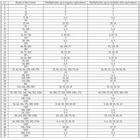
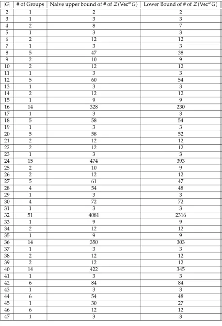
Dω G. Using this link, a classification of the simple objects inZ(VecωG)and formulas for the modular data ofZ(VecωG)are carefully derived. Then, code is written in GAP to produce the modular data ofZ(VecωG), givenωandG. This is used to create a database of modular data for the Drinfeld doubles of pointed fusion categories with dimension less than 47. This database as well as GAP code accompanying it can be found athttps://tqft.net/web/research/ students/AngusGruen. For a basic example of how this database might be used, we briefly analyse patterns in the ranks of Z(VecωG)as |G|varies and produce lower bounds for the number of Morita equivalence classes of pointed fusion categories of a given dimension less than 47. For dimensions below 32, these lower bounds agree with the lower bounds published by Mignard and Schauenburg in [1]. At dimension 32 we improve upon the published lower bound and for dimensions 33 through 47 we present the first set of lower bounds on the number of Morita equivalence classes of pointed fusion categories at each dimension.
Contents
Acknowledgements v
Abstract vii
1 Introduction 1
2 Preliminaries 3
2.1 Monoidal Category Theory . . . 3
2.1.1 Pivotal and Braided Categories . . . 5
2.1.2 String Diagrams . . . 7
2.1.3 Fusion and Modular Categories . . . 10
2.1.4 The Drinfeld centre . . . 13
2.2 Backgroup Algebra . . . 15
2.2.1 Group Cohomology . . . 15
2.2.2 Hopf Algebras . . . 15
2.2.3 Representation Theory of Hopf Algebras . . . 18
2.2.4 Projective Representation Theory . . . 22
3 Classifying equivalence classes of Pointed Fusion Categories 27 3.1 TwistedG-graded Vector Spaces . . . 27
3.2 Functors betweenVecαGandVecβH . . . 29
3.3 Equivalence classes of Pointed Fusion Categories . . . 33
4 Modular Data for the Drinfeld Centre of TwistedG-graded Vector Spaces 37 4.1 An Intricate Hopf Algebra . . . 38
4.2 The Modular Equivalence between Rep(DωG)andZ(Vecω−1)bop . . . 40
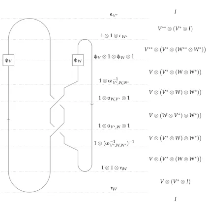
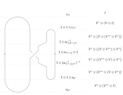
4.3 Deriving the S and T matrices forZ(Vecω−1)bop . . . 47
4.3.1 Classifying the Simple Objects . . . 47
4.3.2 Deriving the S Matrix . . . 48
4.3.3 Deriving the T Matrix . . . 53
5 Computing Modular Data in GAP 57 5.1 Choosing a Set of 3-cocycles . . . 58
5.2 Computing the Simple Objects . . . 58
5.3 Computing the S and T Matrices . . . 61
6 Analysis of Modular Data 65
A Group Cohomology 69
B More Code 71
Chapter 1
Introduction
Fusion categories are an important area of study due both to their frequent occurrence in category theory as well as their applications in physics. An important current area of study in low-energy physics is the study of a phenomenon called “topological phases of matter”. These topological phases are potentially key components in technological advancements in areas such as superconductors and quantum computing. One approach to studying topological phases of matter is through modelling them with topological quantum field theories (TQFTs). The cobordism hypothesis [2] states that TQFTs are classified by higher categorical data and in particular the work of Douglas–Schommer-Pries–Snyder [3] identifies fully extended TQFTs in 2+1 dimensions1with fusion categories.
Pointed fusion categories are a particular class of fusion categories possessing several useful properties. These categories are classified by pairs(G,ω)of a finite groupGand a 3-cocycleω
onG. In addition, the Drinfeld centre of a pointed fusion category turns out to be equivalent to a representation category of a Hopf algebra known as the twisted quantum double of the group
G. This correspondence allows for categorical problems to be translated over into algebraic problems which can then be solved by algebraic means.
This thesis is broadly split into three parts. Chapter 2 gives an overview of the background category and algebra theory. In particular the category theory section builds up to the definition of a modular category and gives an overview of the Drinfeld centre construction. The back-ground algebra focuses on giving an introduction to Hopf algebra theory and a slightly unusual perspective on projective representation theory.
Chapters 3 and 4 focus on finding the equivalence classes of pointed fusion categories and the corresponding modular data. Chapter 3 introduces the category ofG-graded vector spaces VecωGand explains how they are naturally pointed fusion categories. It then details the equiv-alence classes of these categories by proving a theorem classifying the functors between two such categories. Chapter 4 introduces the twisted quantum doubles of a finite groupDωG, and proves an equivalence of modular tensor categories between Rep DωG
andZ Vecω−1Gbop
. Using this equivalence, we give a detailed derivation for the modular data ofZ Vecω−1Gbop
and explain the link between this modular data and the modular data ofZ Vecω−1G
.
Finally, Chapters 5 and 6 focus on the computational aspects of the project. Chapter 5 describes the code written to compute the modular data ofZ Vecω−1Gbop
givenGandω. In particular it discusses the methods used to create a list of simple objects ofZ Vecω−1Gbop
and the various optimisations used to speed up the calculations of theSandTmatrices from this list. Then, a database of this modular data will be assembled for all equivalence classes of pointed fusion categories with dimension at most 47. Code written by Micha¨el Mignard and Peter Schauenburg in their recent paper [1] is used to find a list of unitary 3-cocycles which are a representatives of a representative cohomology class of each orbit inH3(G,C)/Aut(G).
1We write 2+1 as opposed to 3 to specify that there are 2 spatial dimensions and 1 time dimension.
Then, given a group G and a unitary 3-cocycleω my code constructs the modular data of
Z Vecω−1Gbop
. Chapter 6 will then focus on some results that can be derived from this database. In particular we confirm the result of Mignard and Schauenburg concerning the number of Morita equivalence classes of pointed fusion categories at each dimension less than 32, improve upon their lower bound when the dimension is equal to 32 and publish new lower bounds at each dimension between 33 and 47 inclusive. We note that the improvement at dimension 32 also proves that the modular data of a category is a stronger invariant than the Frobenius-Schur indicators andT-matrix.
The classification of functorsVecαG→VecβGin Chapter 3 is technically new but presum-ably obvious to experts. Cain Edie-Michell is about to publish a classification of equivalences of graded categories [4]. My result is neither a special case as it classifies more than just the equivalence classes, nor as strong as it only covers the case when the trivial graded piece isVec.
A careful derivation of the equivalence Rep DωG ∼
= Z Vecω−1Gbop
has not been pub-lished before. In particular, no-one seems to have noticed that with the usual conventions you are required to invert both the associator and the braiding. While the formulas pre-sented for theSandTmatrices do appear in the literature [5], the corresponding derivations of these formulas do not. These derivations are given in careful detail in Section 4.3. The database of modular data constructed as described in Chapter 5 is available for public use at
Chapter 2
Preliminaries
More in-depth discussions on the definitions in this section can be found in the textbook Tensor Categories [7].
2.1
Monoidal Category Theory
Definition 2.1. A monoidal category(C,⊗,I,α,λ,ρ)consists of a categoryC along with a bifunctor ⊗:C ×C →C, an identified object I, and three natural isomorphismsα,λ,andρ. The associatorα, has components
αX,Y,Z :(X⊗Y)⊗Z−→∼ X⊗(Y⊗Z) ∀X,Y,Z∈C and the left and right unitorsλandρ, have components
λX :I⊗X−→∼ X
ρX:X⊗I −→∼ X ∀X∈C.
These natural transformations satisfy the following commutative diagrams for all W,X,Y,Z∈ C.
(W⊗X)⊗(Y⊗Z)
(W⊗X)⊗Y
⊗Z W⊗ X⊗(Y⊗Z)
W⊗(X⊗Y)
⊗Z W⊗ (X⊗Y)⊗Z
αW,X,Y⊗Z
αW⊗X,Y,Z
αW,X,Y⊗1Z
αW,X⊗Y,Z
1W⊗αX,Y,Z
(2.1)
(X⊗I)⊗Y X⊗(I⊗Y)
X⊗Y αX,I,Y
ρX⊗1Y
1X⊗λY
(2.2)
If all three ofα,λ, andρcorrespond to the identity natural transformation, then the category is called strict. A monoidal category is an example of a process known as categorification. Recall that a monoid consists of a setS, with an function∗:S×S→ Ssatisfying(a∗b)∗c=a∗(b∗c) for alla,b,c ∈ Ssuch that there exists a unique elemente ∈ Ssuch thata∗e = e∗a = afor everya ∈ S. Categorification takes a set theoretic definition and replaces sets by categories, functions by functors and equations by natural transformations satisfying certain commutative diagrams. Then a monoidal category is a categorification of a monoid. Similarly, many of the following definitions will be categorifications of more well known structures.
Theorem 2.2(Mac Lane’s Coherence Theorem). In a monoidal category, any diagram with edges consisting only of tensor products ofα,λ,ρ, and identity morphisms is commutative.
Proof. See [8].
Given two monoidal categories (C,⊗,I,α,λ,ρ) and(D,·,J,β,κ,µ), a monoidal functor between them is as follows.
Definition 2.3. A monoidal functor(F,Φ,φ)consists of a functor F :C → Dalong with a natural isomorphism called the tensorator,
ΦX,Y: F(X)·F(Y)−→∼ F(X⊗Y) ∀X,Y∈Ob(C)
and an isomorphism
φ∈D(J −→∼ F(I)).
There are three commutative diagrams that these transformations must satisfy.
(F(X)·F(Y))·F(Z) F(X)·(F(Y)·F(Z))
(F(X⊗Y))·F(Z) F(X)·(F(Y⊗Z))
F((X⊗Y)⊗Z) F(X⊗(Y⊗Z))
βF(X),F(Y),F(Z)
ΦX,Y⊗1Z 1X⊗ΦY,Z
ΦX⊗Y,Z ΦX,Y⊗Z
F(αX,Y,Z)
(2.3)
J·F(X) F(I)·F(X)
F(X) F(I⊗X)
φ⊗1X
κF(X) ΦI,X
F(λX)
(2.4)
F(X)·J F(X)·F(I)
F(X) F(X⊗I)
1X⊗φ
µF(X) ΦX,I
F(ρX)
(2.5)
These three commutative diagrams are each relating a structure inC with the corresponding structure in D. Commutative Diagram 2.3 relates the two associators and the other two commutative diagrams relate the left unitors and right unitors respectively. This definition is a categorification of a monoid homomorphism. Unlike monoids, there is another layer that can be placed on top of monoidal functors. Given two monoidal functors(F,Φ,φ)and(G,Θ,θ) from(C,⊗,I,α,λ,ρ)to(D,·,J,β,κ,µ), there can be monoidal natural transformations between them.
Definition 2.4. A monoidal natural transformationη, is a natural transformation from F→G which satisfies the following commutative diagrams.
F(X)·F(Y) G(X)·G(Y)
F(X⊗Y) G(X⊗Y)
ηX⊗ηY
ΦX,Y ΘX,Y
ηX⊗Y
§2.1 Monoidal Category Theory 5
J
F(I) G(I)
φ
θ
ηI
(2.7)
In general, most of the monoidal categories that we work with have additional structures or properties on top of just a monoidal structure. For this thesis we will need to define a modular tensor category. Expanding this prefix, a modular tensor category is a finitely semisimple pivotal braided linear monoidal category with a simple unit and an invertibleSmatrix. The next couple of subsections will be devoted to explaining each of these prefixes.
2.1.1 Pivotal and Braided Categories
LetC be a monoidal category.
Definition 2.5. A right dual of an object X ∈C is an object X∗ ∈C with an evaluation map
X:X∗⊗X→I and a co-evaluation map
ηX :I →X⊗X∗.
These maps must satisfy the condition that compositions1
X−−−→ηX⊗1X X⊗X∗⊗X −−−→1X⊗X X X∗−−−−→1X∗⊗ηX X∗⊗X⊗X∗ −−−−→X⊗1X∗ X∗ are both the identity.
While right duals are not unique, they are unique up to unique isomorphism [7]. There is a related notion of left dual,∗Xwhich can be elegantly defined as an object inC which hasXas a right dual.
Definition 2.6. The categoryC is a rigid monoidal category if every object has both a left and a right dual.
In a rigid category, for any objectXit should be clear that∗X∗ ∼=X.
It is also possible to take the dual of a morphism. Given a morphism f ∈C(X→Y), f∗is a morphism inC(Y∗ →X∗)defined by the composition
Y∗ 1Y∗⊗ηX
−−−−→Y∗⊗X⊗X∗ −−−−−−→1Y∗⊗f⊗1X∗ Y∗⊗Y⊗X∗ −−−−→Y⊗1X∗
X∗.
The morphism∗f is similarly defined as
∗
Y−−−−−−→η∗X⊗1∗Y⊗ ∗X⊗X⊗∗Y−−−−−−→1∗X⊗f⊗1∗Y ∗X⊗Y⊗∗Y−−−−→1∗X⊗∗Y ∗X.
Observe that the two conditions on compositions given in the definition of∗are exactly stating that(1X)∗ = 1X∗and∗(1X) =1∗X. There are two features of these definition that I will state
without proof here. These proofs are a little verbose currently but will become almost trivial when using string diagrams which will be introduced in the next section.
1We implicitly assume that the monoidal categoryC is strict for this definition. There is a similar but more
Lemma 2.7. The dual operator on morphisms satisfies∗f∗ = f and(f◦g)∗ =g∗◦ f∗.
Another property of the dual operator is that it flips monoidal products. If XandYare objects with right duals X∗ and Y∗ respectively then(X⊗Y)∗ ∼= Y∗⊗X∗. The evaluation and co-evaluation maps are given byX⊗Y =Y◦(1⊗X⊗1)andηX⊗Y= (1⊗ηX⊗1)◦ηY
respectively.
This leads to the following important lemma.
Lemma 2.8. The dual operator is an op-monoidal contravariant functor.
Briefly, a contravariant functor F : C → D is a mapping between two categories which flips morphisms. This means that for eachX∈C,F(X)is an object inD but, unlike a regular functor2, if f ∈ C(X → Y) then F(f) ∈ C(F(Y) → F(X)). This mapping is required to satisfy the pair of equationsF(1X) =1F(X)andF(f◦g) = F(g)◦F(f). Then, an op-monoidal
functor is almost a monoidal functor except the op-tensorator is a natural transformation from
F(Y)·F(X)−→∼ F(X⊗Y).
The proof of Lemma 2.8 is immediate from Lemma 2.7 and the discussions preceding and ensuing it.3
A slightly stronger notion than duals is that of invertible objects.
Definition 2.9. An object X is said to be invertible if X∗⊗X∼= X⊗X∗ ∼= I.
Clearly if this is the case,X∗is also invertible andX∼= X∗∗. More generally, it is often useful to require an isomorphism betweenXand its double dual. This requires extra structure on the category called a pivotal isomorphism.
Definition 2.10. A pivotal monoidal category is a pair(C,φ)withC a rigid monoidal category andφ
a monoidal natural isomorphism from the identity functor to the double dual functor, [9].
Observe that the composition of two op-monoidal contravariant functors is a monoidal functor. Hence the double dual functor is indeed a monoidal functor fromC to itself and so
φis well defined. The pivotal isomorphism also gives an isomorphism betweenX∗ and∗X. Therefore, in a pivotal categoryX∗can be unambiguously referred to as the dual ofX.
Definition 2.11. A braided monoidal category(C,σ)consists of a monoidal categoryC with a natural isomorphism
σX,Y: X⊗Y→Y⊗X such that the following diagrams commute.
(X⊗Y)⊗Z X⊗(Y⊗Z) (Y⊗Z)⊗X
(Y⊗X)⊗Z Y⊗(X⊗Z) Y⊗(Z⊗X)
αX,Y,Z
σX,Y⊗1Z
σX,Y⊗Z
αY,Z,X
αY,X,Z 1Y⊗σX,Z
(2.8)
X⊗(Y⊗Z) (X⊗Y)⊗Z Z⊗(X⊗Y)
X⊗(Z⊗Y) (X⊗Z)⊗Y (Z⊗X)⊗Y α−1X,Y,Z
1X⊗σY,Z
σX⊗Y,Z
α−1Z,X,Y α−1X,Z,Y σX,Z⊗1Y
(2.9)
A braiding on a monoidal category is a categorification of commutativity.
2These are commonly called covariant functors when in situations where contravariant functors also appear. 3Once again we have implicitly assumed thatCis strict. Everything remains true ifCis not a strict monoidal
§2.1 Monoidal Category Theory 7
2.1.2 String Diagrams
String diagrams are a method of representing information in a category in terms of a graphical calculus of planar diagrams. By convention, strings are read going up the page.
Definition 2.12. Given a morphism f : A→B its string diagram is
A f B
points correspond to objects and morphisms correspond to boxes on lines connecting two points.
Composition of morphisms f,his vertical stacking and the tensor product is horizontal juxtaposition.
h◦f
A C
=
f h
A B
C
A B
f
A0 B0
g =
A A0 B B0
f ⊗g =
A⊗A0 B⊗B0
f ⊗g
There is a slight abuse of notation here. For a category with no extra structure, a string diagram is really referring to the equivalence class of string diagrams up to a certain planar isotopies. The allowed isotopies change as more structures and properties are added to the categories. Currently, we are allowed to slide the morphism boxes around as if they were beads on the string and move the strings so long as the end points are fixed, no part of a string is ever horizontal and strings do not cross each other.
Various special morphisms are assigned particular diagrams. A simple example is that an empty string, with no boxes, crossings, or horizontal tangents corresponds to the identity morphism. Often an identity morphism is unambiguously referred to as the object itself. More interesting examples occur when the category has additional structures. For example, if the category is braided then the braiding and inverse braiding are represented by over and under crossings diagrams.
σV⊗W =
V W
V W
σV−⊗1W =
W V
W V
If the category is rigid then the evaluation and co-evaluation morphisms are represented by the following strings.
V V∗
V = ηV =
V∗ V
Note that in this picture, the line corresponding to 1Ias well as the point Ihave been replaced
by empty space. When the unitors in the category are trivial,4this can be done with no loss of information. This serves to simplify diagrams, the morphismV◦ηVis
V◦1I◦ηV =
V V∗
V∗ V
=
V V∗
V∗ V
=V◦ηV.
Another problem is what to do with associators. When the category is strict, they can be safely ignored, however this will not be possible for this thesis. On the other hand including them will massively clutter the string diagrams. Therefore, they will be omitted from string diagrams throughout and this will mean that some care will need to be taken reading morphisms directly off string diagrams. Note that by Theorem 2.2, any two morphisms read off the same string diagram are equal.5
When the category is rigid, there is also a convenient way to represent dual objects. This is by assigning directions to the lines with the convention that a line travelling up the page corresponds to the object and one travelling down the page corresponds to its right dual. Then, the the conditions on theandηcorrespond to the following isotopies.
= =
As a brief justification for the use of string diagrams let us go back and prove Lemma 2.7.
4Which they will be for this thesis.
5We need to be a little careful here. This holds provided the initial and final bracketing of the objects is unchanged
§2.1 Monoidal Category Theory 9
Proof. Observe that the two morphisms f∗and∗f are defined by the following strings
f∗
Y∗
X∗
Y∗ X∗
= f ∗f
∗Y ∗X = ∗X ∗Y f
Then, the following isotopies of string diagrams shows that∗f∗ = f.
∗f∗
∗X∗ ∼=X
∗Y∗ ∼=Y
= f∗
X Y = f X Y = f X Y = f X Y
Similarly, different isotopies prove that(f◦g)∗ =g∗◦ f∗
X∗ g∗◦f∗
Z∗ = f∗ g∗ X∗ Y∗ Z∗ = X∗
f Y∗
g Z∗ = X∗ f Y g Z∗ = X∗ f Y g Z∗ = X∗ f ◦g
Z∗
=
X∗
(f◦g)∗
Z∗
If the category is pivotal, the pivotal isomorphism allows for the creation of closed loops. This gives rise to the definition of a trace. Given a morphism f ∈C(V→V)define the left and right traces of f to be
f
φV
trL(f) =
φ−V1
f
These are morphisms inC(I → I). Commonly,C(I → I)will be isomorphic to a fieldKand
when this is the case, a trace corresponds to an evaluation map fromC(V→V)→K. InVec, the category of finite dimensional vector spaces with morphisms linear maps, the trace of a morphism is exactly the trace of the matrix representing the morphism after a basis is chosen.
Definition 2.13. A pivotal monoidal category is spherical if all string diagrams behave as if they where on the surface of a sphere, [9]. Equivalently,trL(f) =trR(f)for all f .
In particular in a spherical category, strings can be pulled around the back of the sphere which identifies the two possible traces.6 In a spherical category, the dimension of an object is
defined to be the trace of the identity.
dim(V) =tr(1V)
Combining all the structure and properties that have been defined so far brings us to ribbon categories.
Definition 2.14. A ribbon category is a braided spherical monoidal category.
These categories possess a twist mapθVfor each object satisfying
θV⊗W =σV,WσW,V(θV⊗θW).
This map is defined by the string diagram
φV θV =
V
V∗
V∗∗
.
The proof that this morphism satisfies the alleged condition is easily shown using string manipulations and so will be omitted. The reason that these are called ribbon categories is because, if one-dimensional strings are replaced by ribbons embedded in 3-space,θcan be represented by a full twist in the ribbon.
2.1.3 Fusion and Modular Categories
Definition 2.15. Given a fieldK, aK-linear category is a categoryC whose morphism spacesC(X→ Y)areK-vector spaces with the composition map being bilinear.
Any K-algebra is naturally aK-linear category with a single object. More generally, a K-linear category is equivalent to a K-algebroid. A linear functor is a functor whose action
on morphism spaces corresponds to a linear map. All functors whose source and target are linear categories will be assumed to be linear functors. If an endomorphism space End(X) = C(X →X)is one dimensional, it must be generated by the identity morphism 1Xand so, as
F(1X) =1F(X), the action of a linear functorFon End(X)is determined by its action onX.
6Pulling a string around the back of a sphere will possibly invertφor have other small effects like sendingη
Vto
§2.1 Monoidal Category Theory 11
Definition 2.16. An initial object is an object X ∈ C such that for all Y ∈ C,C(X →Y)contains only one element. Similarly, X is a terminal object if for all Y ∈ C,C(Y → X)contains only one element.
Lemma 2.17. Initial and terminal objects are unique up to isomorphism.
Proof. This is a standard result in category theory, a proof can be found in [8] for the interested reader.
An object that is both initial and terminal is said to be a zero object and by Lemma 2.17 this is also unique up to isomorphism. In aK-linear category, these conditions exactly require that
C(X→Y)is the 0 dimensional vector space,{0}.
Definition 2.18. AK-linear category with a0object is semisimple if there exists a collection of objects {Xi}i∈I called the simple objects with the following set of properties:
1. For all i and j in I,
C(Xi →Xj) =
(
K if i= j {0} otherwise.
2. All finite coproducts exists.
3. Any object X ∈C is isomorphic to a (possibly infinite or null) direct sum of simple objects.
An object which is isomorphic to a finite direct sum of simple objects is called finitely semisimple. A semisimple category is said to be finitely semisimple if every object is finitely semisimple and there are only finitely many isomorphism classes of simple objects.
When a category is semisimple this often allows for analysis of the category to be restricted to merely analysing the simple objects. This comes from the fact that many of the structures that can be placed on a category respect these decompositions. For example, if a semisimple category has a monoidal structure, then the associator will satisfy
αW⊕X,Y,Z=αW,Y,Z⊕αX,Y,Z.
This feature of semisimple categories will be implicitly used throughout this thesis as it will massively simplify proofs. Additionally, functors whose sources and targets are semisimple categories will also respect such decompositions
F(X⊕Y) =F(X)⊕F(Y).
Definition 2.19. A fusion category is a finitely semisimple rigid linear monoidal category such that the unit object I is simple.
This thesis will focus on a particular subclass of fusion categories called pointed fusion categories.
Definition 2.20. A pointed fusion category is a fusion category such that every simple object is invertible.
can define a dimension of the category. To find dim(C), choose a representativeVifrom each
isomorphism class of simple objects and then7
dim(C) =
∑
i
dim(Vi)2.
IfC is a ribbon category then there is a matrix we can construct by taking traces of the double braiding applied to pairs of simple objects.
Definition 2.21. LetC be a ribbon fusion category with simple objects{Vi}for i∈ {1,· · · ,n}. Define
theS matrix by the string diagram˜
˜
Si,j =
Vi Vj
ThenC is a modular tensor category ifS is invertible.˜
The matrix ˜Sis also known as the unnormalisedS-matrix. The normalisedS-matrix,S, is equal to √ 1
dim(C)
˜
S.
There is a second matrix that can be created from a modular tensor category. By definition, for every simple objectVi,C(Vi → Vi) =K. Therefore, the twistθV is some multiple of the
identity idVi defined asti.
θVi = ti
Then, theTmatrix is defined to be the diagonal matrix withi’th diagonal element equal toti.
Taking a trace,Tcan be calculated by evaluating the string diagram
Ti,j = dimδi(,jV i)
Vi∗
Vi∗
Vi∗∗ Vi
In general, the matrix produced by this would also need to be normalised however, in this thesis we only deal with categories where the normalisation factor is 1. For a modular tensor categoryC, the pair of matricesS,Tis known as the modular data.
The reason that it is called modular data is because it gives a representation of the modular group SL(2,Z)by way of the map
0 −1
1 0
7→ S and
1 1 0 1
7→T.
7It is an easy proof that this definition is independent of the chosen representatives; isomorphic objects have
§2.1 Monoidal Category Theory 13
This means that the modular data must satisfy the relations S2 = (ST)3 and S4 = I and in practise it also satisfies more complex relations [10] which I will discuss in more detail in Chapter 5.
2.1.4 The Drinfeld centre
The Drinfeld centre [11] is an operation that takes a monoidal category C and produces a braided monoidal category denotedZ(C). OftenZ(C)is referred to as the centre ofC. The construction of the Drinfeld centre is as follows.
Let(C,⊗,I,α,λ,ρ)be a monoidal category. Fixing any objectX∈C, a half braiding forX
is a natural isomorphismβ:X⊗ −→∼ ⊗Xsuch that
βY⊗Z
X Y⊗Z
Y⊗Z X
=
βY βZ
X Y⊗Z X Y⊗Z
Writing this out as a condition on morphisms, the condition is
αY−,1Z,X◦(1⊗βZ)◦αY,X,Z◦(βY⊗1)◦αX−,1Y,Z =βY⊗Z. (2.10)
Then, objects of Z(C) are pairs (X,β) of X an object in C and β a half braiding for X. Morphisms inZ(C)are morphisms inC that commute with the half braidings. Explicitly,
f ∈ Z(C) (X,β)→(Y,γ)if and only if f ∈C(X→Y)and
f
γZ
X Z
Y Z
=
βZ
f
X Z
Y Z
for allZ∈C. The monoidal structure onZ(C)is8
(X,β)⊗(Y,γ) = (X⊗Y,α ,X,Y◦(β⊗1)◦α−X,1 ,Y◦(1⊗γ)◦αX,Y, ). (2.11)
The identity object is simply (I,λ◦ρ−1)and the left and right unitors and associator come directly from the categoryC. Observe that the action of the tensor product on half braidings is
8The blank sections are where the object to be twisted should appear. E.g. if given a Z ∈ C the natural
exactly given by the string diagram
(β⊗γ)Z
X⊗Y Z
Z X⊗Y
=
γZ βZ
X⊗Y Z X⊗Y Z
Theorem 2.22. The Drinfeld centre of a category can be made into a braided monoidal category.
Proof. The easiest way to prove this theorem is to produce a braiding. Hence define the braiding
σby
σ(X,β),(Y,γ) =βY.
Note that
σ(0X,β),(Y,γ) =γ−X1 =σ(−1
Y,γ),(X,β)
is another possible braiding. A priorineither of these braidings is the correct one to ascribe and, as we will observe later, in our particular case we will use the inverse braiding. Note thatZ(C) will refer to the regular braiding andZ(C)bopwill refer to the inverse braiding.9
It is of course required to show that these braidings both satisfy the relevant commutative diagrams, namely Diagrams 2.8 and 2.9. But, these follow directly from the fact that half braidings satisfy Equation 2.10 and by the definition of how the tensor product acts on half braidings given in Equation 2.11.
An important aspect of the Drinfeld centre is that it preserves both the monoidal properties ofC as well as any added monoidal structures onC.
Theorem 2.23. IfC is rigid, pivotal, spherical or fusion then so isZ(C). In particular ifC is a spherical fusion category thenZ(C)is a modular tensor category.
The proof of this theorem is outside the scope of this thesis but can be found in [12] for an interested reader. In particular it is important to note that both rigidity and pivotality can be directly induced by the corresponding properties and structures onZ(C). Interestingly, while it is certainly true that equivalent categories have equivalent centres, the converse is not true.
Definition 2.24. Two monoidal categoriesC andDare said to be Morita equivalent ifZ(C)∼=Z(D).
Note that Morita equivalence is a weaker condition than equivalence of categories this is shown explicitly by Figure 6.2. It should also be noted that there is a relationship between the dimension of the category and the dimension of its centre. Indeed we have the simple formula
dim(Z(C)) =dim(C)2.
There is not however a well understood relationship between the rank of a category and the rank of its centre. This will be explored briefly in Chapter 6.
9bop stands for opposite braiding andCbopis a well defined category wheneverC is braided. We can similarly
§2.2 Backgroup Algebra 15
2.2
Backgroup Algebra
2.2.1 Group Cohomology
There is a small amount of group cohomology that will be useful later and so is given here. LetGbe a finite group with identitye and letKbe an algebraically closed field. Define Cn(G,
K)to be the group under pointwise multiplication of all functions fromGn →K×. Note
that these functions are nota priorirequired to interact withG’s group structure. Define the maps∂n+1 :Cn(G,K)→Cn+1(G,K)by
∂n+1(φ)(g1,· · · ,gn+1) =φ(g2,· · · ,gn+1) ×
n
∏
i=1φ(g1,· · · ,gi−1,gigi+1,gi+2,· · · ,gn+1)(−1)
i
(2.12)
×φ(g1,· · · ,gn)(−1) n+1
.
Theorem 2.25. The sequence
· · · Cn+1 dn+1 Cn dn Cn−1 · · · (2.13)
is a cochain complex.
This is a standard result in group cohomology, see [13]. Define Zn(G,
K) = ker(dn+1), Bn(G,K) = Im(dn)and Hn(G,K) = Zn(G,K)/Bn(G,K).
Elements ofCn(G,K)are known asn-cochains, elements ofZn(G,K)asn-cocycles and elements
ofBn(G,K)asn-coboundaries.
Definition 2.26. Two cocycles,α,β, are cohomologous ifαβ−1is a coboundary. A cocycle is cohomo-logically trivial if it is cohomologous to the1cocycle or equivalently if it is a coboundary.
Definition 2.27. A normalized cochain is a cochain which outputs1whenever any of its inputs are e.
Definition 2.28. A normalized cochainαis unitary ifα|G| =1.
This leads up to the theorem that will be needed later on.
Theorem 2.29. Every cocycle is cohomologous to a unitary cocycle.
Proof. See Appendix A.
2.2.2 Hopf Algebras
For any finite groupGits representations form a category known as Rep(G). The objects of this category are representations ofGand the morphisms are intertwining maps. Moreover, there is a natural equivalence between Rep(G)and Rep(K[G]), the category of representations of the group algebraK[G]. It is well known that Rep(G)carries much more structure than
merely a category. Indeed, Rep(G)is a ribbon fusion category whose simple objects correspond to the irreducible representations ofG. A natural question then is if this extra structure on Rep(G) ∼= Rep(K[G]) can be visualised down in the algebra K[G]. Indeed it can be and
corresponds to added structures onK[G]such as co-multiplication, and an antipode. The
general term for algebras with these two extra structures is a Hopf algebra and representations of Hopf Algebras naturally form rigid monoidal categories.
can be replaced by algebraic ones which allow for a wealth more methods to simplify and solve them. The following sections will give an introduction to Hopf algebras and their representation categories. For more discussion on the structures presented here, see [14].
LetKbe an algebraically closed field and assume for the rest of the section that all maps are Klinear and all tensor products are overK. Initially letHbe aKvector space.
Definition 2.30. An algebra is a triple(H,η,∇)where
η:K→ H ∇: H⊗H→ H
satisfy the commutative diagrams.
H⊗H⊗H H⊗H
H⊗H H
∇⊗1
1⊗∇ ∇
∇
K⊗H∼= H∼= H⊗K H⊗H
H⊗H H
1⊗η
η⊗1 1 ∇
∇
The first commutative diagram is precisely forcing the multiplication map to be associative and the second commutative diagram is forcing a multiplicative identity,η(1).
Define F : H1⊗H2 → H2⊗H1 to be the flip map F(x⊗y) = y⊗x. An algebra is
commutative if∇ = ∇ ◦F. Given two algebras,(H1,η1,∇1),(H2,η2,∇2), there is a natural
algebra structure onH1⊗H2given by H1⊗H2,η1⊗η2,(∇1⊗ ∇2)◦(1⊗F⊗1)
.
Moving on, a coalgebra is defined by reversing every arrow in the definition of an algebra.
Definition 2.31. A coalgebra is a triple(H,,∆)where
:H→K ∆: H→H⊗H satisfy the commutative diagrams
H H⊗H
H⊗H H⊗H⊗H
∆
∆ 1⊗∆
∆⊗1
H H⊗H
H⊗H K⊗H∼= H∼= H⊗K
∆
∆ 1 1⊗
⊗1
Similarly to the algebra case, the first commutative diagram represents coassociativity and, cocommutativity occurs if∆ = F◦∆. Additionally, if (H1,1,∆1)and(H2,2,∆2)are
coalgebras then the tensor product coalgebra will be H1⊗H2,1⊗2,(1⊗F⊗1)◦(∆1⊗∆2). A bialgebra is a vector space with algebra and a coalgebra structures(η,∇)and(,∆)such that bothηand∇are coalgebra homomorphisms and bothand∆are algebra homomorphisms.
Definition 2.32. A bialgebra is a tuple(H,η,∇,,∆)such that(H,η,∇)is an algebra,(H,,∆)is a coalgebra and the following four diagrams commute.
H⊗H H H⊗H
H⊗H⊗H⊗H H⊗H⊗H⊗H
∇
∆⊗∆
∆
1⊗F⊗1
§2.2 Backgroup Algebra 17
K H
K 1 η
(2.15)
H⊗H H
K⊗K∼=K
∇
⊗
(2.16)
K⊗K∼=K
H⊗H H
η⊗η
η
∆
(2.17)
The tensor product structure on algebras and coalgebras defined earlier extends to bialgebras in the obvious way.
A Hopf algebra is a bialgebra with an extra map called an antipode.
Definition 2.33. A Hopf algebra is a pair(H,S)where H is a bialgebra and S an automorphism of H such that the following diagram commutes
H⊗H H⊗H
H K H
H⊗H H⊗H
S⊗1
∇
∆
∆
η
1⊗S
∇
(2.18)
The tensor product of two Hopf algebras(H1,S1)and(H2,S2)is the Hopf algebra(H1⊗ H2,S1⊗S2). In general it is too much to ask for Hopf algebras to be cocommutative but there
is a weaker notion known as almost cocommutative that uses the algebra structure onH⊗H.
Definition 2.34. A Hopf algebra H, is almost cocommutative if there exists an invertible element R∈ H⊗H such that
∆op(h) = F◦∆(h) =R∆(h)R−1 (2.19)
for all h∈ H.
Note that∇has been omitted in the above equations for clarity and for the same reason will be omitted from here on out.
Define the mapsφi j : H⊗H→ H⊗H⊗Hby
φ12(a⊗b) =a⊗b⊗1
φ13(a⊗b) =a⊗1⊗b
φ23(a⊗b) =1⊗a⊗b. Additionally, defineRi j =φi j(R).
Definition 2.35. A quasitriangular Hopf algebra is an almost cocommutative Hopf algebra such that
(∆⊗1)(R) =R13R23 (2.20)
It can also occur that the coproduct is not coassociative. Again if there is an algebra structure it is possible to weaken coassociativity to allow for it to fail up to conjugation by an invertible element.
Definition 2.36. A quasi bialgebra is a tuple(H,,∆,Φ,l,r)with H an algebra andΦis an invertible element of H⊗H⊗H satisfying the following equations for every h∈H.
(∆⊗1)◦∆(h) =Φ (1⊗∆)◦∆(h)
Φ−1 (2.22)
h
1⊗1⊗∆(Φ)ih ∆⊗1⊗1
(Φ)i= (1⊗Φ)h 1⊗∆⊗1
(Φ)i(Φ⊗1) (2.23)
(⊗1)(∆(h)) =l−1hl (2.24)
(1⊗)(∆(h)) =r−1hr (2.25)
1⊗⊗1(Φ) =1⊗1 (2.26)
For the purposes of this thesis assume thatl=r=1. This will simplify some proofs later on. In particular it makes the unitors in the representation category of a quasi bialgebra trivial. Also note thatΦ−1will also satisfy Equations 2.23 and 2.26.
Definition 2.37. A quasi Hopf algebra is a tuple(H,S,α,β)with H a quasi bialgebra,α,β∈ H and S:H →H satisfying the following conditions. Let∆(h) =∑ihi1 ⊗hi2,Φ=∑iXi1⊗Xi2 ⊗Xi3 and
Φ−1 =∑iYi1⊗Yi2⊗Yi3, then we require that
∑
iXi1βS(Xi2)αXi3 =1
∑
iS(Yi1)αYi2βS(Yi3) =1
and for all h∈ H,
∑
iS(hi1)αhi2 =(h)α
∑
ihi1βS(hi2) =(h)β.
The quasitriangular structure can also be extended to quasi Hopf algebras.
Definition 2.38. A quasitriangular quasi Hopf algebra is a tuple(H,R)with H a quasi Hopf algebra and R and invertible element in H⊗H satisfying
∆op(h) = F◦∆(h) =R∆(h)R−1 for all h∈ H and
(∆⊗1)R=Φ321R13Φ−1321R23Φ123 (2.27)
(1⊗∆)R=Φ−2311R13Φ213R12Φ−1231 (2.28)
whereΦabc =∑iXia⊗Xib⊗XicandΦ123=Φ=∑iXi1⊗Xi2 ⊗Xi3
2.2.3 Representation Theory of Hopf Algebras
Definition 2.39. A representation of an algebra H is a vector space V with an algebra homomorphism
§2.2 Backgroup Algebra 19
Thisρcan either be thought of as a map H → (V → V)or a map H×V → V. With the second interpretation, a representation is exactly the same as a left module. Note that,ρbeing an algebra homomorphism, means thatρ(h1)◦ρ(h2) = ρ ∇(h1,h2)
and for allk ∈ K, and
v∈V,ρ(η(k),v) =kv.
Let Rep(H) be the category whose objects are representations of H and morphisms are intertwining maps. Equivalently, from the above interpretation, Rep(H)can be thought of as the category whose objects are left modules with morphisms module homomorphisms. These two points of view will be used interchangeably.
Theorem 2.40. If H is a quasitriangular quasi Hopf algebra thenRep(H)is a rigid braided monoidal category.
While ideally this thesis would prove the above theorem, in practise the proof would be far too lengthy. Instead we will prove the following three lemmas which combine to a slightly weaker theorem. It should however be clear in the proofs of these lemma’s how they could be extended to stronger statements so as to prove the above theorem.
Lemma 2.41. If H is a quasi bialgebra thenRep(H)is a monoidal category.
Lemma 2.42. If H is a Hopf algebra then the antipode S givesRep(H)the property of a rigid monoidal category.
Lemma 2.43. If H is a quasitriangular Hopf algebra then the quasitriangular element induces a braiding onRep(H).
Note that Lemmas 2.42 and 2.43 assume that the underlying coalgebra is coassociative.
Proof of Lemma 2.41. Let(U,ρ), (V,σ)and (W,τ)be representations of H. Initially we must construct the tensor product of representations. ClearlyU⊗Vis a representation of H⊗H
via the mapρ⊗σ. In order to make this a representation of H, recall that the coproduct
∆ is an algebra homomorphism. Hence define(U,ρ)⊗(V,σ) = U⊗V,(ρ⊗σ)◦∆. An easy calculation checks that if f : U → W and g : V → X are intertwining maps, then
f ⊗g:U⊗V →W⊗Xis also an intertwining map.
The identity object is exactly (K,)and the isomorphisms(K,)⊗(V,σ) −→∼ (V,σ)and (V,σ)⊗(K,) −→∼ (V,σ) follow from Equations 2.24 and 2.25 after the simplification that
l=r= 1.
This leaves us to define the associator. The two possible tensor products of the three representations are10
(U,ρ)⊗(V,σ)
⊗(W,τ) = U⊗V⊗W,(ρ⊗σ⊗τ)◦(∆⊗1)◦∆
and
(U,ρ)⊗ (V,σ)⊗(W,τ)
= U⊗V⊗W,(ρ⊗σ⊗τ)◦(1⊗∆)◦∆
Recall that there is an identified elementΦ∈ H⊗H⊗Hsatisfying (∆⊗1)◦∆(h) =Φ (1⊗∆)◦∆(h)
Φ−1.
Therefore,
(ρ⊗σ⊗τ)(Φ−1)◦(ρ⊗σ⊗τ) (∆⊗1)◦∆(h)
= (ρ⊗σ⊗τ)Φ−1 (∆⊗1)◦∆(h)
10Note that we are working here with a model ofVecwhere the monoidal structure is strict. If our model ofVec
= (ρ⊗σ⊗τ) (1⊗∆)◦∆(h)
Φ−1
= (ρ⊗σ⊗τ) (1⊗∆)◦∆(h)
◦(ρ⊗σ⊗τ)(Φ−1).
This means thatαρ,σ,τ = (ρ⊗σ⊗τ)(Φ−1)is an intertwining map
αρ,σ,τ :
(U,ρ)⊗(V,ψ)⊗(W,φ)→(U,ρ)⊗(V,ψ)⊗(W,φ).
Moreover, Equation 2.23 directly forcesα to satisfy Commutative Diagram 2.1 and, as the unitors are trivial Equation 2.26 shows thatαwill satisfy Commutative Diagram 2.2. Therefore
αis an and so with these structures,(Rep(H),⊗,(K,),α, 1, 1)is a monoidal category.
It is unfortunate that in the definition ofα,Φ−1is used instead ofΦ. This is the commonly used notation in the field but will cause some trouble later on. Moving on, we next wish to prove that for a Hopf algebraH, Rep(H)is rigid.
Proof of Lemma 2.42. Note that a bialgebra is equivalent to a quasi bialgebra withΦ=1⊗1⊗1 andl=r=1. Thus, the previous proof gives us a strict monoidal structure on Rep(H).
Let(V,ρ)be an object in Rep(H). Define a new object(V∗,ρ∗)whereV∗is the vector space dual ofVand, for allh∈ H, f ∈V∗andm∈V,
ρ∗(h, f)(m) = f ρ(S(h),m)
.
Claim: This constructed object(V∗,ρ∗)is the dual object of(V,ρ).
LetγVbe the usual linear mapV∗⊗V→Kand recall that the action ofHonV∗⊗Vand
Kis given by(ρ∗⊗ρ)◦∆andrespectively. Then the following computation shows thatγV
commutes with the action ofH.
γV◦ (ρ∗⊗ρ)◦∆(h)
(f⊗m) =
∑
i
γV◦ (ρ∗⊗ρ)(hi1⊗hi2)(f⊗m)
=
∑
i
γV
ρ∗(hi1, f)⊗ρ(hi2,m)
=
∑
i
ρ∗(hi1, f)
ρ(hi2,m)
=
∑
i
fρ S(hi1),ρ(hi2,m)
= f◦ρ◦(S⊗ρ)◦(∆⊗1)(h,m)
= f◦ρ◦(1⊗ρ)◦(S⊗1⊗1)◦(∆⊗1)(h,m)
= f◦ρ◦(∇ ⊗1)◦(S⊗1⊗1)◦(∆⊗1)(h,m) ∗
= f◦ρ◦ (η◦)⊗1
(h,m) ∗∗
=(h)f(m) ∗ ∗ ∗
=(h)◦γV(f⊗m)
Note that the steps∗and∗ ∗ ∗are simple using the definition ofρas an algebra homomorphism and in particular in∗ ∗ ∗ observing that(h) ∈ K. Then, step∗∗ is a direct consequence of Commutative Diagram 2.18. In order for(V∗,ρ∗)to be the dual, there also needs to be a map from(K,)→(V,ρ)⊗(V∗,ρ∗). Again, we can use the regular vector space mapζV, which is, for a basis{vi}ofVwith corresponding basis{v∗i}ofV∗
ζV(1) =1
∑
i
§2.2 Backgroup Algebra 21
A calculation no worse than the above will show thatζVcommutes with the action ofH. This shows that every element has a right dual. An identical argument will also show that every element must have a left dual and so Rep(H)is a rigid monoidal category.
In the case whereHis only a quasi Hopf algebra, theαandβin Definition 2.37 increase the complexity of the evaluation and co-evaluation maps. For the right dual of a left module (V,ρ), the evaluation mapγVis replaced byγV◦(1⊗ρ(α))and the co-evaluation mapζVwill be replaced by(1⊗ρ∗(β))◦ζV. Similar modifications will be made to the regular vector space structures for left duals. Next, consider the case when the the Hopf algebra is quasitriangular. This will allow us to assign a braiding to Rep(H).
Proof of Lemma 2.43. Let H be a quasitriangular Hopf algebra. This means that there is an invertibleR∈ H⊗Hsuch thatF◦∆(h) =R∆(h)R−1andRsatisfies Equations 2.20 and 2.21.
Let (V,ρ)and (W,τ) be elements of Rep(H)with the strict monoidal structure defined earlier. Then, a braiding will be an isomorphism between V⊗W,(ρ⊗τ)◦∆ and W⊗ V,(τ ⊗ρ)◦∆
. Using the flip mapF, we have∀h ∈H, w∈W, v∈Vthe equality
(τ⊗ρ)◦∆(h)
(w,v) =F◦(ρ⊗τ)◦F◦∆(h)◦F(w,v) = F◦(ρ⊗τ)(R∆(h)R−1)◦(w,v)
= F◦(ρ⊗τ)(R)◦(ρ⊗τ)(∆(h))◦ F◦(ρ⊗τ)(R)−1
(w,v).
Rewriting this gives
F◦(ρ⊗τ)(R)◦(ρ⊗τ)(∆(h))◦(v,w) = (τ ⊗ρ)◦∆(h)
◦F◦(ρ⊗τ)(R)(v,w). (2.29)
This shows thatσρ,τ = F◦(ρ⊗τ)(R)is an isomorphism
σρ,τ : V⊗W,(ρ⊗τ)◦∆
∼
−→ W⊗V,(τ⊗ρ)◦∆.
In order forσto be a braiding it needs to satisfy Commutative Diagrams 2.8 and 2.9 (These give conditions on how the braiding needs to interact with the tensor product and associators.).
Let(U,ψ),(V,ρ)and(W,τ)be three objects in Rep(H). Then, as the associators are trivial, Commutative Diagram 2.8 requires the equality
(1⊗σψ,τ)◦(σψ,ρ⊗1) =σψ,(ρ⊗τ)◦∆
Equation 2.21 states that
(1⊗∆)R=R13R12 = (F⊗1)
1⊗R×(R⊗1).
Therefore,
σψ,(ρ⊗τ)◦∆= F◦ψ⊗ (ρ⊗τ)◦∆
(R)
= (1⊗F)◦(F⊗1)◦ψ⊗ρ⊗τ)(1⊗∆)(R) = (1⊗F)◦(F⊗1)◦(ψ⊗ρ⊗τ)(R13R12)
= (1⊗F)◦(F⊗1)◦(ψ⊗ρ⊗τ)(R13)◦(ψ⊗ρ⊗τ)(R12) = (1⊗F)◦(F⊗1)◦ (ψ⊗ρ⊗τ)◦(F⊗1)(1⊗R)
=1⊗ F◦(ψ⊗τ)(R)
◦(F⊗1)◦ F◦(ψ⊗ρ)(R)
⊗1 = (1⊗σψ,τ)◦(σψ,ρ⊗1).
The key step in this proof is the observation that
(F⊗1)◦ (ψ⊗ρ⊗τ)◦(F⊗1)(1⊗R)= (ρ⊗ψ⊗τ)(1⊗R)◦(F⊗1). The idea is essentially that(F⊗1)can be pulled through the action (ψ⊗ρ⊗τ)◦(F⊗1)
(1⊗ R)
and act upon each component permuting(ψ⊗ρ⊗τ)7→(ρ⊗ψ⊗τ)and(F⊗1)(1⊗R)7→
(F⊗1)◦(F⊗1)(1⊗R) = (1⊗R).
Therefore as required,σ satisfies Diagram 2.8. A very similar calculation using Equation 2.20 will show thatσ also satisfies Diagram 2.9. For brevity this calculation will be skipped.
Thereforeσis indeed a valid braiding and so(Rep(H),σ)is a braided tensor category.
In the more general case whenHis a quasitriangular quasi Hopf algebra, Equations 2.20 and 2.21 will be replaced by Equations 2.27 and 2.28. Looking at these new equations, it should be clear that they are exactly taking into account the non trivial cocycle. Hence, in the general case the braiding will still be given byσ as defined above.
2.2.4 Projective Representation Theory
This section is based on the paper “A Character Theory for Projective Representations of Finite Groups” by Chuangxun Cheng [15].
LetGbe a finite group, letVbe a complex vector space and letβbe a unitary 2-cocycle. Recall GL(V)and PGL(V); the first is the ring End(V)and the second is GL(V)/C. WhereC
is naturally identified with the subring of End(V)of multiples of the identity map.
Definition 2.44. Aβ-projective representation is a pair(V,ρ)with V a vector space andρa function
ρ:G→GL(V)satisfying
ρ(g)ρ(h) =β(g,h)ρ(gh)
Asβis a 2-cocycleρis associative butρis clearly not a group homomorphism whenβ6=1. This is a slightly unusual definition of a projective representation. In general, a projective representation is defined as a group homomorphism G → PGL(V). For our purposes this second definition is unsatisfactory because we care about the value of the 2-cocycleβ. When mapped through to PGL(V), constants disappear and as such there would be no difference between different values ofβ.
As an example of the difference between these perspectives, consider the case whenG=
Z/2Z = {0, 1}. If we view projective representations as a map to PGL(V), the only one
dimensional projective representation is the trivial one. However, there are non trivial one dimensionalβ-projective representations. For example whenβis given byβ(1, 1) =−1 and all other pairs map to 1, two projective representations are given by 17→iand 17→ −i.
Much of classical representation theory carries across to projective representations. This includes the following definitions and results, stated here without proof. Proofs of these theorems can be found in [15].
Definition 2.45. Two projective representations(V,ρ),(W,ψ)are linearly equivalent if there exists an isomorphism f :V→W such that f ◦ρ(g) =ψ(g)◦ f for all g∈ G.
§2.2 Backgroup Algebra 23
β-projective representations ofZ/2Zgiven a moment ago are examples of representations that
are projectively but not linearly equivalent.
Definition 2.46. Given twoβ-projective representations(V,ρ),(W,ψ), we can form a newβ-projective representation(V⊕W,ρ⊕ψ)called the direct sum.
Theorem 2.47. Let (V,ρ) be a β-projective representation and W ⊂ V a G invariant subspace. Then(V,ρ)can be decomposed into the direct sum of twoβ-projective representations,(W,ρ|W)and
(W0,ρ|W0)where W⊕W0 =V andρ|W represents the action ofρon V restricted to W.
Definition 2.48. A projective representation (V,ρ)is said to be irreducible if the only G invariant subspaces are V and{0}.
Theorem 2.49. All projective representations can be decomposed into a direct sum of irreducible representations. This decomposition is unique up to reordering and linear equivalences.
Definition 2.50. Given a projective representation, the characterχρof the representation is defined to be
χρ(g) =tr ρ(g)
.
Theorem 2.51. Aβ-projective representation is entirely determined by its character.
Note that unlike classical representation theory,χρ(g)need not be constant across conjugacy
classes. Indeed a simple calculation shows that for aβ-projective representation
χρ(hgh−1) =tr ρ(hgh−1)
= 1
β(h,g)β(hg,h−1)tr ρ(h)ρ(g)ρ(h
−1)
= 1
β(h,g)β(hg,h−1)tr ρ(g)ρ(h
−1)ρ(h)
= β(h −1,h)
β(h,g)β(hg,h−1)χρ(g).
Another calculation that will be useful later is the relationship betweenχρ(g)andχρ(g−1).
In order to prove this we will first prove that the eigenvalues ofχρ(g)must be roots of unity.
Letn< ∞be the order ofg. Then
I =ρ(1) =ρ(gn) =β(g,gn−1)−1· · ·β(g,g)−1ρ(g)n. Asβis unitary,β|G| =1 and so
I = I|G| =ρ(g)n|G|.
Therefore the eigenvalues ofρ(g)must be roots of unity which means that the eigenvalues of
ρ(g)−1are the complex conjugates of the eigenvalues ofρ(g). Thus asρ(g)ρ(g−1) =α(g,g−1)I
we find that
χρ(g−1) =tr ρ(g−1)
=tr(α(g,g−1)ρ(g)−1) =α(g,g−1)tr(ρ(g)−1) =α(g,g−1)χρ∗(g−1), (2.30) whereχ∗ denotes the complex conjugate ofχ.
Theorem 2.52. Let G be a group andβa unitary2-cocycle. Then there exists a group Gβcalled the group extension of G and an injective map f fromβ-projective representations of G to linear representations of Gβ.
Proof. First to constructGβ. Asβis unitary it takes values in the group of|G|’th roots of unity in C. This group is naturally identified withA=C|G| = hx|x|G|iby the isomorphisme
2πi
|G| 7→ x. Let
˜
βbe image ofβunder the isomorphism into A. As a set,Gβ= G×Aand its group structure
comes from a twisted multiplication map
(g,xn)×(h,xm) = (gh, ˜β(g,h)xn+m).
Associativity of the multiplication follows from the associativity of the multiplication inGand
Aas well as the 2-cocycle condition whichβsatisfies. Asβis normalized, there is an identity element(e, 1), and inverses are given by(g,xm)−1 = (g−1, β(g,g−1)−1
x−m. This proves that
Gβis indeed a group.
Note that Ais isomorphic to the normal subgroup ofGβgenerated by(e,x)and thatGis
not a subgroup ofGβbut is a quotient group given byG= Gβ/A.
Next let(V,ρ)be someβ-projective representation ofG. Define f(ρ):Gβ→GL(V)by
f(ρ) g,xm
=e2|mGπ|iρ(g).
The following calculation shows that(V, f(ρ))is indeed a linear representation ofGβ.
f(ρ) g,xm
f(ρ) h,xn
=e2 (m+n)πi
|G| ρ(g)ρ(h)
=β(g,h)e2 (m+n)πi
|G| ρ(gh)
= f(ρ) gh, ˜β(g,h)xn+m
= f(ρ) (g,m)×(h,m)
.
The injectivity of f is immediate from noting that f(ρ) g, 1
= ρ(g)and this completes the proof of Theorem 2.52.
An important corollary of this theorem is as follows.
Corollary 2.53. Theβ-projective representation(V,ρ)will be irreducible if and only if(V,f(ρ))is an irreducible linear representation.
Proof. LetW be a Gβ invariant subspace of V. Then as f(ρ) g, 1
= ρ(g), W must also be a G invariant subspace. Conversely, assume that W is not a Gβ invariant subspace. Then
there exists some elementw∈Wand(g,xm)∈ Gβsuch that f(ρ) g,xm)
(w)∈/W. Therefore
ρ(g)(w) = e−2|Gm|π f(ρ) g,xm)(w) ∈/ W and soW is not a Ginvariant subspace. Therefore G
invariant subspaces ofVcorrespond toGβinvariant subspace ofV.
Importantly for us, when looking atβ-irreducible representations this map f has a well behaved inverse on Im(f). It is also easy to check if an irreducible representation ofGβis in
Im(f).
Let(V,ρ)be an irreducible linear representation ofGβ. AsA∼= h(e,x)iis in the center of Gβandx|A| =1, Schur’s Lemma gives us thatρ(e,x) =e
2kπi |A| I
nfor some integerk. Then define
f0(ρ)(g) =ρ(g, 1). Note that f0(f(ρ0)) =ρ0and so
§2.2 Backgroup Algebra 25
Clearly, f0will be aβ-projective representation if and only ifk=1 and, when restricted to such representations f(f0(ρ)) =ρ. Additionally, there turns out to be an easy check to see ifk =1 using characters, as this is equivalent to asking if χ(χ(ee,1,x)) =e2|Aπ|i.
This gives us a method of producing theβ-character table ofGonly using linear represen-tations. First we construct Gβ and find its character table. Then we create a subtable of all
characters that satisfy χ(χ(1,e,1x)) =e2|Aπ|i. Restricting this subtable toG, Corollary 2.53 shows that this
is exactly theβ-character table ofG. This exact method has been encoded intoGAPand the code will be displayed in chapter 5.
One final observation is that, as with linear representations,β-projective representations can also be viewed as left modules of an algebra. Whenβ=1, it is well known that representations ofGare equivalent to left modules ofK[G]. Recall that elements ofK[G]are sums∑g∈Gagg
with eachagsome constant inKand multiplication is defined by
∑
g∈Gagg
∑
h∈Gbhh
=
∑
k∈G
∑
gh=kagbh
k.
This is exactly the linearised version of multiplication in G. More generally, β-projective representations can be viewed as left modules of the twisted group algebra Kβ[G] whose
underlying vector space is identical but multiplication is twisted byβ. That is to sayg×h=
β(g,h)ghor for a more general element
∑
g∈Gagg
∑
h∈Gbhh=
∑
k∈G
∑
gh=kβ(g,h)agbh
k.
The proof of the equivalence betweenβ-projective representations ofGand left modules of
Chapter 3
Classifying equivalence classes of
Pointed Fusion Categories
There exists the following well known theorem about pointed fusion categories.
Theorem 3.1. All pointed fusion categories are equivalent toVecαG for some group G and3-cocycle,α.
Proof. See [16].
This allows us to restrict the problem of studying the equivalence classes of pointed fusion categories to these concrete examples. This chapter will explain what these categoriesVecαG
are and prove several theorems that will allow further restrictions on the equivalence classes of these categories.
3.1
Twisted
G-graded Vector Spaces
Fix a field K, which we suppress for the rest of the chapter and let Gbe a finite group. A G-graded vector spaceVis a vector space which can be decomposed into a direct sum of vector spaces each sitting over a different element ofG
V= M
g∈G
Vg.
Given twoG-graded vector spacesVandW, aG-graded homomorphismψ:V→Wis a linear map that respects theGgrading. This means that for allg ∈ G, the restriction ofψtoVgis a
linear map fromψg:Vg →Wg.
Definition 3.2. The categoryVecG is a skeletal category whose objects are G-graded vector spaces and morphisms are G-graded homomorphisms.
Lemma 3.3. The categoryVecG is linear and semisimple.
Proof. ClearlyVecGis linear as there is a natural vector space structure onG-graded homomor-phisms. Explicitly, for allr,s∈Kandρ,ψ∈ VecG(V →W),(rρ+sψ)is defined by
(rρ+sψ)(v) =rρ(v) +sψ(v).
Bilinearity of the composition map follows from the linearity of morphisms. To prove semisim-plicity define the objectsδgfor eachg ∈Gto be the one dimensionalG−graded vector spaces
(δg)h=
(
K ifh= g {0} ifh6=g.
Observe that ifg6=hthen as(δg)h = (δh)g={0}, the only element ofVecG(δg→δh)is 0. On
the other hand, as(δg)g =K, maps fromδg →δg are identified by their action on(δg)g =K.
Hence End(δg) ∼= Kwith the identification 1δg 7→ 1. Then the composition map in End(δg)
corresponds to multiplication inK. Additionally, it should be clear that everyG-graded vector
spacesV, is isomorphic to a direct sum of these objects as
V∼= M
g∈G |Vg|
M
i=1
δg.
ThereforeVecGis a linear and semisimple category.
Consider the following tensor product onVecG. LettingV,W ∈VecG, defineV⊗W to be theG-graded vector space withg’th component
(V⊗W)g= M
hk=g
Vh⊗Wk.
This tensor product is defined similarly on morphisms. In order to create a monoidal category, this proposed tensor product must admit an associator and there must exist a unit object and unital morphisms. The unit object is clearlyδebut there is more choice in the rest of the structures. Letαbe a natural isomorphism
αX,Y,Z:(X⊗Y)⊗Z−→∼ X⊗(Y⊗Z). AsGis a group, its multiplication is associative and so
(δg⊗δh)⊗δk =δ(gh)k =δg(hk) =δg⊗(δh⊗δk).
As End(δghk)∼=K, for any tuple(g,h,k)∈ G×G×G,αg,h,k is1some scalar inK. Hence, when
restricted to only simple objects,α is exactly a map fromG×G×G → K×. Then, setting
W = δg,X = δh,Y =δk andZ = δl, Commutative Diagram 2.1 (The commutative diagram equating the two possible maps from(((W⊗X)⊗Y)⊗Z→W⊗(X⊗(Y⊗Z))) is an equality in End(δghkl)which corresponds to the equality inK
αh,k,lαg,hk,lαg,h,k =αgh,k,lαg,h,kl.
Asαis uniquely defined by its action on the simple objects, the above equation implies that there is a bijection between possible associators and 3-cocycles inZ3(G,K). We can classify the
possible unitors using a similar method. SettingX=δgandY=δh, Commutative Diagram 2.2 (The commutative diagram equating the two possible maps from(X⊗I)⊗Y → X⊗Y) corresponds to the equality
ρg =αg,e,hλh.
Fixλe = k ∈ K×and observe that the 3-cocycle condition on the tuple(e,e,e,e)forces that
αe,e,e=1. Then, as the above equation is satisfied for allg,h, this means thatρe =λe =kand more generally all of theλ’s andρ’s on simple objects can be written in terms ofαandk
ρg=kαg,e,e (3.1)
1For simplicity, whenever we subscriptαor more generally any natural transformation by group elements, this
§3.2 Functors betweenVecαGandVecβH 29
λh= k
αe,e,h. (3.2)
While all possible choices ofkproduce different monoidal categories it can be easily proven that these categories are all monoidally equivalent. Forαa 3-cocycle andk ∈K×, letVecα
kG
denote the monoidal category of G graded vector spaces whose associator on the simple objects corresponds to multiplication byαand unitors on the simple objects corresponds to multiplication byρandλas defined in Equations 3.1 and 3.2. Additionally, defineVecαG= Vecα1G. Note that there is a mild abuse of notation here in thatαwill be simultaneously referred to both as a 3-cocycle and as the associator.
Lemma 3.4. The categoriesVecαkG andVecαG are equivalent monoidal categories.
Proof. Consider the monoidal functor(F,Φ,φ)fromVecαGtoVecαkGwithFthe identity functor,
Φthe identity natural transformation andφmultiplication bykinK∼=End(I). It is a simple
check to confirm that these definitions satisfy Commutative Diagrams 2.3, 2.4, and 2.5. Therefore this defines a monoidal functor which is clearly invertible and so the two categoriesVecαkGand VecαGare equivalent monoidal categories.
The following theorem will be stated without proof; the proof is provided later on in the chapter as a more complete understanding of the monoidal equivalence classes ofVecαGis required.
Theorem 3.5. The monoidal categoriesVecαG are pointed fusion categories.
One method of describing monoidal equivalence classes is to first understand the possible functors that can occur between categories.
3.2
Functors between
Vec
αG
and
Vec
βH
This section will focus on the proof of Theorem 3.6. This theorem is certainly known to experts in the field but I have been unable to find a citation with either a proof or a statement of it.
Theorem 3.6. There is a bijection between the monoidal functors fromVecαG→VecβH up to monoidal natural isomorphism and the set
(θ,Γ)|θ∈Hom(G→ H),Γ ∈ H2
G,K×; α
β·θ
.
The notationβ·θ refers to the function defined byβ·θ(g,h,k) = β(θ(g),θ(h),θ(k))for
g,h,k∈ G. Additionally,H2G,
K×;βα·θ
is the relative homology ofGwith respect to βα·θ. This
is defined as(∂3)−1
α β·θ
modulo the relationx∼ yifxy−1 ∈Im ∂2.
The proof of this theorem will be the combination of the following four lemmas. The first two show thatH2G,
K×;βα·θ
is well defined and the second two are proving the bijection.
Lemma 3.7. Givenβa 3-cocycle on H and a group homomorphismθfrom G to H,β·θis a 3-cocycle on G.
Lemma 3.8. Let Φ ∈ (∂3)−1
α β·θ
andγ ∈ Im ∂2. Then Φγ ∈ (∂3)−1
α β·θ