Extending the coverage area of regional ionosphere maps using a support vector machine algorithm

https://doi.org/10.5194/angeo-37-77-2019 © Author(s) 2019. This work is distributed under the Creative Commons Attribution 4.0 License.

Extending the coverage area of regional ionosphere maps using a

support vector machine algorithm

Mingyu Kim and Jeongrae Kim

School of Aerospace and Mechanical Engineering, Korea Aerospace University, Goyang-si, 10540, Korea Correspondence:Jeongrae Kim ([email protected])

Received: 7 September 2018 – Discussion started: 25 September 2018

Revised: 9 January 2019 – Accepted: 17 January 2019 – Published: 31 January 2019

Abstract. The coverage of regional ionosphere maps is de-termined by the distribution of ground-based monitoring sta-tions, e.g., GNSS receivers. Since ionospheric delay has a high spatial correlation, ionosphere map coverage can be ex-tended using spatial extrapolation methods. This paper pro-poses a support vector machine (SVM) to extrapolate the ionosphere map data with solar and geomagnetic parame-ters. One year of IGS ionospheric delay map data over South Korea is used to train the SVM algorithm. Subsequently, 1 month of ionospheric delay data outside the input data re-gion is estimated. In addition to solar and geomagnetic en-vironmental parameters, the ionospheric delay data from the inner data region are used to estimate the ionospheric delay data for the outside region. The accuracy evaluation is per-formed at three levels of range−5, 10, and 15◦_{outside the}

inner data regions. The extrapolation errors are 0.33 TECU (total electron content unit) for the 5◦region and 1.95 TECU for the 15◦region. These values are substantially lower than the GPS Klobuchar model error values. Comparison with an-other machine learning extrapolation method, the neural net-work, shows a substantial improvement of up to 26.7 %.

1 Introduction

Ionospheric delay is one of the main error sources for single-frequency global navigation satellite system (GNSS) re-ceivers. Ionosphere models or ionosphere maps can be used to correct for ionospheric delay. For real-time applications, a regional ionosphere map using regional GNSS monitor-ing stations can be used to provide highly accurate correc-tions. The regional ionosphere map coverage is determined by the distribution of GNSS ground-based monitoring

sta-tions. Since ionospheric delay has a high spatial correlation, ionosphere map coverage may be extended by using spatial extrapolation methods. In addition to the spatial correlations, time variables such as observation hour and day number, and solar and geomagnetic indices can serve as input parameters for the extrapolation.

A series of research studies have been conducted on the temporal extrapolation (prediction) of regional ionosphere maps using past observations. With respect to using machine learning algorithms, Kumluca et al. (1999) applied the neural network (NN) method to forecast ionospheric critical plasma frequencies,foF2. McKinnell and Friedrich (2007) used a NN to predict the lower ionosphere in the aurora zone. Okoh et al. (2016) developed a regional vertical total electron con-tent (VTEC) model for Nigeria based on observational data from 12 stations and tested temporal and spatial extrapo-lation performance. Unlike previous studies, the extrapola-tion performance was improved by adding the Internaextrapola-tional Reference Ionosphere (IRI) as an input. Razin and Voosoghi (2016) applied a wavelet NN with particle swarm optimiza-tion to predict the total electron content (TEC) over Iran. Huang and Yuan (2014) used time and temporal variation of the TEC values as radial-basis function (RBF) network inputs to temporal extrapolation. A support vector machine (SVM) model has been used to predict the ionosphericfoF2 above Chinese stations (Ban et al., 2011; Chen et al., 2010). Akhoondzadeh (2013) used a SVM to predict the TEC and to detect seismo-ionospheric anomalous variations.

(2014) applied a biharmonic spline method to extend a small ionospheric correction coverage area. Ionospheric delay ob-servations were used as the input parameters, and the iono-spheric delay outside the coverage area was extrapolated. Le-andro and Santos (2006) used geographical information as inputs of a NN model for spatial extrapolation of TEC over Brazil. For spatial extrapolation, Jayapal and Zain (2016) used a NN with time and solar or geomagnetic indices. In addition to these environmental parameters, Kim and Kim (2016) used the ionospheric delay of the inner area to im-prove the performance of spatial extrapolation.

In addition to the NN method, a SVM algorithm can be considered for spatial extrapolation. A SVM finds a solution to the convex quadratic programming problem in training to optimize the margin so that it can be both optimal and unique. On the other hand, a NN finds the weight between each layer through the gradient descent method, and the solution has a possibility to fall into the local minima in this process. A NN is based on empirical risk minimization (ERM), which is a method of minimizing learning errors during the learning process. On the other hand, a SVM is based on structural risk minimization (SRM), so it has excellent generalization per-formance (Gunn, 1998). SVMs have been widely used as pre-dictive models in various fields. Huang et al. (2015) success-fully performed stock market movement predictions using a SVM. Mohandes et al. (2014) performed wind speed predic-tions using a SVM and compared the performance against the NN method. The results showed that the SVM achieved superior prediction performance.

This paper proposes a SVM algorithm to extend iono-sphere map coverage by applying temporal and environmen-tal parameters and ionospheric observations. The IGS iono-sphere map is used as a reference map, and the extrapolation accuracy of the SVM is evaluated by comparing it to the IGS map data. The extrapolation accuracies are compared with the GPS Klobuchar model and the NN model.

2 Parameter modeling

Three types of input parameters are used for the extrapola-tion of a regional ionosphere map – temporal parameters, en-vironmental parameters, and ionospheric delay observations. An extrapolated ionospheric delay, IDext, may be represented

as a function of these three parameters.

IDext=f (xt xe xobs) , (1)

wherext andxeare the time and the environmental

parame-ters, respectively, andxobsis ionospheric delay observations

in the inner area. The inner area is defined as a geographi-cal area where ionospheric delay information or observations are available. The outer area is defined as a geographical area where ionospheric delay will be estimated.

The ionospheric variation is correlated with the diur-nal and seasodiur-nal time variation, and the ionospheric delay

above the locations involved in the study reaches its maxi-mum around 14:00 local time (LT) and its minimaxi-mum around 02:00 LT (Wu et al., 2012). Also, the daily mean ionospheric delay is higher in spring and autumn, and lower in summer and winter (Wu et al., 2012; Mansoori et al., 2015). In order to adopt these correlations, time parameters are included in the extrapolation model. The diurnal variation is represented by an hour number (00:00–23:00 LT), and the seasonal vari-ation is represented by a day number (0–365). To represent the repeatability of these variations, the time parameters are modeled as sinusoidal functions.

xt=[SD CD SH CH], (2)

whereSDandCDare the sine and cosine, respectively, of the

day number, andSHandCHare the sine and cosine,

respec-tively, of the hour numbers. The periods used for the sinu-soidal functions are set to 24 h and 365.25 days for the di-urnal and seasonal parameters, respectively. The ionosphere activity is also highly correlated with solar and geomagnetic activity. Three parameters are selected to reflect the space environment – the F10.7 index, geomagnetic index Kp, and sunspot number (SSN).

xe=F10.7 Kp SSN (3)

Although SSN has a similarity with F10.7 in representing solar activity, use of both parameters yielded slightly better estimation accuracy than use of single parameter. Therefore, both F10.7 and SSN are adopted for the environmental pa-rameters. Experiments on the selection of optimal solar ac-tivity indices will be discussed in Sect. 5.

Disturbance storm time (Dst) may replace Kp for iono-sphere storm detection but it was not selected. Dst response performance depends on ionosphere storm driver. Dst is ef-ficient for storms driven by coronal mass ejection (CME), but it is less effective for storms driven by corotating interac-tion regions (CIRs) or coronal hole high speed streams (CH HSSs) (Borovsky and Denton, 2006; Denton et al., 2006). After a series of numerical experiments on selecting Dst or Kp, Kp was selected for the parameter because of its better estimation performance. The numerical experiments will be discussed in Sect. 4.

Past inner-area ionospheric delays are used to train the ma-chine learning algorithms, and current inner-area delays are used for the extrapolation. The observation data set for theN

observation points is derived as follows.

xobs= h

with fixed grid points, and their location information is not required as the model inputs.

In the event of high temporal or geographical decorrelation due to geomagnetic storms, two inputs are affected: the solar or geomagnetic parameters and the ionosphere input data in inner region. Because of observation latency, the real-time solar or geomagnetic parameters may not be available in real time. However the ionosphere input data may be available in real time from GPS observations, and this fact makes for the estimation algorithm to respond to the geomagnetic storm in real time.

3 Extrapolation methods

3.1 Support vector machine (SVM)

The SVM method is a machine learning theory that was pro-posed by Vapnik in 1995. It uses an algorithm to find a hy-perplane that maximizes the margin (Gunn, 1998). It is used in data classification and regression problems, and SVMs used in regression are referred to as support vector regres-sion (SVR). A SVM sets the regresregres-sion function,f (xsvm),

such that targetysvmis in the following range.

f (xsvm)= ˆysvm=wTxsvm+b, (5)

f (xsvm)−ε≤ysvm≤f (xsvm)+ε, ε >0, (6)

wherexsvmis the input that contains [xt xe xobs], andwT

is the transposed weighting matrix;ysvmis the target that

rep-resents the true ionospheric delay in the extrapolation region, andxεis the allowable error level forysvm. In many practical

cases,ysvmis not in the range of(f (xsvm)−ε, f (xsvm)+ε),

andysvm is frequently adjusted to the range of(f (xsvm)−

ξ, f (xsvm)+ξ ), whereξ is a slack variable. The optimal

re-gression function is determined when the total magnitude of the slack variable, P

iξi is minimized. Also, the distance between f (xsvm) and the support vector should be

maxi-mized. The distance between the SVM andf (xsvm)is called

the margin, and the margin may also be minimized. There-fore, the optimal regression function minimizes kwkandξ

to achieve the maximum margin (Gunn, 1998).

minkwk

2

2 +C

Xn

i=1 ξ −

i +ξ

+

i

, (7)

subject toysvm−f (xi,svm)−ξi≤ε ifysvm−f (xi,svm)≥ε

ysvm−f (xi,svm)+ξi ≥ −ε, ifysvm−f (xi,svm)≤ −ε (8)

In Eq. (7), the superscript – denotes a lower boundary and +denotes an upper boundary. The slack variable disappears while expanding equations.C is the penalty set by users. As the C value approaches zero, the weight for the slack vari-able decreases and the relative weight for kwk2 increases. Therefore, the regression function that maximizes the margin can be calculated. This implies that the regression function differs fromysvm. AsC increases, the weight for the slack

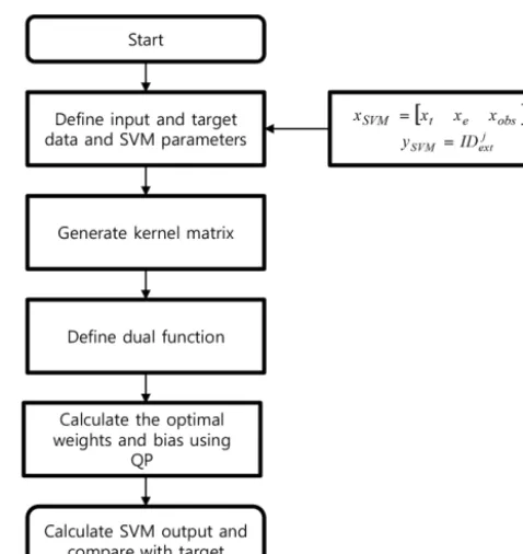
Figure 1.Flow chart of the SVM training process.

variable sum increases rather than maximizing the margin magnitude. Therefore, a regression function is calculated in a form similar toysvm. Equation (7) can be modified using a

dual problem, as follows. arg min

β 1 2β

T_{K x}

i,SVM, xj,SVMβ−fTβ

f= −ysvm+ε, (9)

whereβisα−−α+andαis Lagrange multiplier.Kis a ker-nel function that maps input dataxsvmto a higher dimension.

Kernel functions have several functions, including linear and polynomial functions. The most commonly used functions are Gaussian kernel functions (Cristianini, 2001).

K (xsvm, ysvm)=exp −

k_xsvm−ysvmk2

2σ2 !

(10)

After mappingxsvmto feature space, one can determine the

optimalβ by using quadratic programming (QP). The opti-mal regression function can be computed by using the fol-lowing equation (Gunn, 1998).

f (xsvm)=wTx+b=

XN

i=1β T_{K x}

i,SVM, xj,SVM

+1

n

XN

i=1

XN

j=1 n

yi,SVM−βj∗K xi,SVM, xj,SVM o

(11)

region, and these inputs are identical for each extrapolation point. Targets include the true ionospheric delay in thej-th extrapolation point. After the input and output of the SVM is defined, a kernel matrix is generated for each input. Then, the training is performed to find the optimal coefficients and bias of the regression function,f (xsvm). The kernel function

is calculated for the epoch of each input so that the size of the matrix becomesN×N, whereNis the number of epochs. As the input increases, the computational time and memory us-age also increase. Therefore, the elements of the kernel ma-trix, including the oldest epoch, are deleted, and the kernel functions of the recent epoch are included in the matrix. After defining the kernel function and the boundary of the regres-sion function, the optimal weights and biases are calculated using the interior point method (Ferris and Munson, 2004). When the initial training is completed, the extrapolation and update of the kernel function are repeated.

3.2 Neural network (NN)

A NN is a statistical learning model similar to a biological neural network. It consists of neurons or perceptions, and a synapses. Neurons are interconnected with synapses, which store weights. A NN can solve problems such as pattern recognition and regression by calculating the weights from the learning of the neurons (Habarulema et al., 2011).

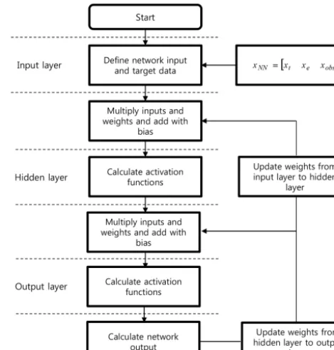
Several types of NNs exist – e.g., back-propagation neu-ral network (BPNN), recurrent neuneu-ral network (RNN), and time delay neural network (TDNN). This study implements a BPNN, which is one of the most commonly used NN algo-rithms. It is a feed-forward, multi-layer perceptron (MLP), supervised learning network (Jwo et al., 2004). In the hidden layer, activation functions determine whether the values from the previous layer are activated or not. Training is generally performed using the gradient descent method.

Figure 2 shows a flow chart of the BPNN used for the regional ionosphere map extrapolation. The input layer in-cludes the network inputs,xNN, shown in Eqs. (2), (3), and

(4). The network inputs and targets are the same as those used in the SVM. An input neuron multiplied by a weight can be computed through the hidden layer towards the output neu-ron, as follows.

ˆ

yNN=fn

Wn,n−1fn−1Wn−1,n−2fn−2 (· · ·f1(W1,0xNN+b1)· · · +bn−2)+bn−1

+bn, (12) wherebis the network bias,nrepresents thenth layer, and

Wn,n−1is the weight fromn−1 to thenth layer;xNN is the

network input, which includes the three input parameters for extrapolation, yˆNN is the network output, andf is an

acti-vation function. The hyperbolic tangent sigmoid function is implemented, which is the most widely used method. The network is trained using the BPNN algorithm with true iono-spheric delays and three input parameter sets to find the op-timal weights and biases.

Figure 2.Flow chart of the neural network training process.

The network data are generally divided into training, vali-dation, and test sets. The training set is used to calculate and update the weights. The validation set is used to verify the training results. The test set is finally used to calculate the extrapolation error. This paper uses three data sets divided by 70 %, 15 %, and 15 %, respectively. A detailed implemen-tation of the NN can be found in Kim and Kim (2016).

4 Data processing

An IGS global ionosphere map (GIM) is used to acquire ref-erence ionospheric delay data because of its high accuracy and global coverage (IGS, 2019). Regional ionospheric de-lay time series are generated with the GIM data, and they are used to train the extrapolation algorithms. The extrap-olated ionospheric delays outside the observation area are compared with the GIM data to evaluate the accuracy. The IGS GIM grid size is 2.5◦×5◦, but other regional ionosphere maps such as the space-based augmentation system (SBAS) ionosphere corrections have an equal latitude–longitude grid size. Therefore, a 5◦_×5◦ _{grid size is used for the regional}

ionosphere map in this research.

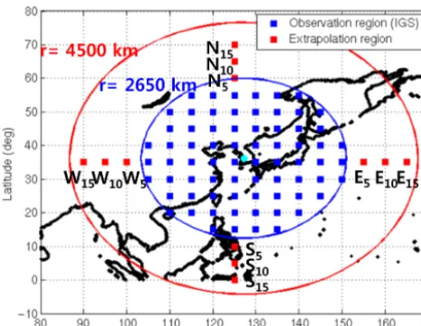
Figure 3.Observation and extrapolation regions of ionospheric de-lay grids.

and the estimation interval is not an important factor for de-termining the accuracy.

Figure 3 illustrates the observation and extrapolation grid points. The observation regions (blue) are set with a radius of 2650 km centered on South Korea, and the extrapolation regions (red) are set with a radius of 4500 km in order to in-clude the 15◦extended grid point from South Korea. There-fore, the latitude of the observation area ranges from 15 to 55◦N, and the longitude ranges from 105 to 150◦E. The ac-curacy evaluation points are selected to perform the extrap-olation. In order to accommodate the directional characteris-tics of the extrapolation performance, the evaluation point set is selected for each direction (north, south, east, and west). In each direction, three points are selected with different dis-tances from the inner observation region:−5, 10, and 15◦. All the locations of the extrapolation points are represented in Table 1.

In the case with the environmental parameters (i.e., F10.7, Kp, and SSN), real-time data may not exist at the extrapola-tion epoch due to data latency. In order to simulate this data latency, previous one-epoch (2 h) values are used instead of the current values during the extrapolation process. This time interval is not large because it is not a temporal prediction method, but a spatial extrapolation method. The influence of the time interval on the estimation performance is much smaller than the ionosphere input data. True environmental parameters are used in the training process, but the previous one-epoch values are used in the extrapolation process. The correlation analysis between the current and previous one-epoch values confirms the correlation. The correlation coef-ficients between the two adjacent epochs of data for F10.7, Kp, and SSN are 0.930, 0.863, and 0.852, respectively. Since the IGS GIM uses 2 h intervals, the Kp, which is provided every 3 h, is interpolated at intervals of 2 h.

Figure 4.One-year variation of ionospheric delay (1 October 2013 to 30 October 2014, S15 (south 15◦point)).

Previous research showed that extrapolation errors have a high correlation with the ionospheric delay magnitude and variation (Kim and Kim, 2014). Therefore, the high iono-spheric delay season is more appropriate when evaluating the extrapolation algorithm than the low ionospheric delay sea-son. It means that if the magnitude of the ionospheric delay and variation is small, all the extrapolation values and errors are small. In this case, it is difficult to compare the extrap-olation performance for each model. The training period is set to 1 year from 1 October 2013 to 30 September 2014. In this period, the minimum and maximum ionospheric delays are 5.1 and 112.2 TECU (total electron content unit), respec-tively, as shown in Fig. 4. The extrapolation period is set to 1 month from 1 to 31 October 2014. The region analyzed in this paper is located around the midlatitudes. In this region, the ionospheric spatial gradient is large in the north–south direction. Also, since the southern area is close to the geo-magnetic equator, its ionospheric variation is very large.

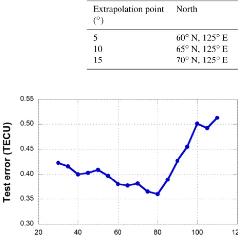
The training and extrapolation performance depend on user parameters. In the case of the NN, extrapolation per-formance mainly depends on the number of hidden neurons. If the number of hidden neurons is too high, over-fitting may occur, and the calculation time is long. Since there are no criteria for determining the number of hidden neurons, the optimal number of hidden neurons must be found by ana-lyzing the extrapolation error variation due to the number of neurons. The model parameters with the lowest test error are adopted as the optimal values. In Figs. 5 and 6, test errors are computed by the mean RMS extrapolation errors at the 5◦ _{extrapolation regions. In case of the NN, the number of}

Table 1.The locations of the extrapolation points.

Extrapolation point North East South West (◦)

5 60◦N, 125◦E 35◦N, 155◦E 10◦N, 125◦E 35◦N, 100◦E 10 65◦N, 125◦E 35◦N, 160◦E 5◦N, 125◦E 35◦N, 95◦E 15 70◦N, 125◦E 35◦N, 165◦E 0◦N, 125◦E 35◦N, 90◦E

Figure 5.Test errors of different numbers of hidden neurons by the NN model (5◦extrapolation point).

error to determine the lowest extrapolation error case. They are set to 10−6and 10−7, respectively.

In order to select an ionospheric storm-related input pa-rameter between Kp and Dst, a series of experiments was performed by replacing Kp with Dst. The experiments con-cluded that Kp is better for our estimation algorithm than Dst. After replacing Kp with Dst, both the SVM and NN estima-tion accuracies were degraded. At 5◦ extrapolation points, the SVM estimation error was increased from 0.33 TECU (Kp) to 0.44 TECU (Dst) and the NN estimation error was increased from 0.45 to 0.63 TECU. Similar levels of error increases were observed at both the 10 and 15◦points. The NN accuracy degradation with Dst was more significant dur-ing high ionospheric disturbance period, when Dst <−25 nT (9, 19–21, 28 October). However only 1 month of data is tested in this research. One month may not be sufficient for evaluating the estimation performance under various iono-sphere conditions, e.g., CME-, CIR-, or CH HSS-related ionospheric disturbances. Comprehensive analysis with a longer data period, e.g., multiple years, can be a further re-search topic.

5 Results

The regional ionosphere map extrapolation is performed us-ing the SVM, and the IGS GIM is used as a truth value. The SVM extrapolation results are compared with the NN and Klobuchar model results. Hourly variations of the

extrapo-Figure 6.Test errors of differentCvalues by the SVM model (5◦ extrapolation point).

lation results are analyzed with 1-day data, and then daily variations of the results are analyzed with 1-month data.

5.1 Single-day extrapolation analysis

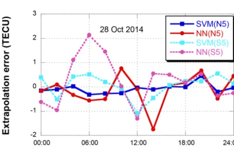
The variations of the ionospheric delay and the extrapolation results are analyzed for the data from 28 October 2014, when the daily ionospheric delay magnitude reaches its maximum for the extrapolation period (October 2014).

Figure 7 shows the ionospheric delay variations of the IGS GIM and Klobuchar model on 28 October 2014. Data from two evaluation points, 5◦north and south, are presented. Uni-versal time (UT) is used. The ionospheric delay reaches its maximum at 15:00 LT (06:00 UT) and then decreases. There are large differences between the ionospheric delays at the north and south points because of the ionospheric spatial gradient (Kim et al., 2014). The north–south difference pro-duced by the Klobuchar model is significantly smaller than the IGS GIM.

de-Figure 7.Ionospheric delays of the IGS GIM and Klobuchar model (south 5◦and north 5◦points).

Figure 8.Extrapolation error variations on 28 October 2014 (north 5◦and south 5◦points).

lay variation. The NN error at N5 and SVM errors at S5 and N5 do not follow the ionospheric delay variation.

Figure 9 compares the RMS errors of four 5◦extrapolation points (N5, S5, E5, and W5) on 28 October 2014. The error magnitude is the largest at the south point where the iono-spheric delay magnitude is the largest. The SVM shows sim-ilar error levels for the north, east, and west points. However, the NN shows larger errors than the SVM even at the north point. This difference in extrapolation accuracy may be ex-plained via the ionospheric spatial gradient. The spatial gra-dient along the north–south direction is significantly greater than the gradient along the east–west direction (Kim et al., 2014; Vukovi´c and Kos, 2016). The large gradient increases the geographical ionospheric delay difference and frequently causes the NN error increase. However, the SVM is more robust for this large amount of gradient data. In general iono-sphere estimation errors increase at low geomagnetic latitude (Song et al., 2018). However, the errors at E5 and W5 are smaller than those at N5 point even though E5 and W5 are located to the south of N5. This is because the input of the model includes the internal ionospheric delay for solving a

Figure 9.Extrapolation errors for each direction (5◦extrapolation regions).

Figure 10.Extrapolation errors for each direction (10◦ extrapola-tion regions).

spatial extrapolation problem. It implies that the ionospheric spatial gradient is the main factor of the extrapolation perfor-mances.

Figure 10 compares the RMS errors of four 10◦ extrapola-tion points (N10, S10, E10, and W10) on 28 October 2014. Unlike the 5◦ results in Fig. 7, there is little difference be-tween the two models for the northern area. However, the difference between the two models in the southern region is increased to 0.63 TECU. It means that the extrapolation per-formance of the SVM and the NN model is larger for the high ionospheric variation region. The extrapolation errors of the east and west region are not significantly different from those in Fig. 9.

Figure 11 compares the RMS errors of four 15◦

be-Figure 11.Extrapolation errors for each direction (15◦ extrapola-tion regions).

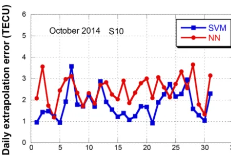
Figure 12. Daily extrapolation RMS error variations in October 2014 (south 10◦point).

comes diminished. Therefore, the accuracy difference be-tween SVM and NN has been reduced.

5.2 One-month extrapolation analysis

The spatial extrapolations are performed for the 1-month pe-riod from 1 to 31 October 2014. As with the single-day ex-trapolation, the 1-year data from October 2013 to September 2014 are used for the training process.

Figure 12 shows the daily extrapolation errors for the south 10◦extrapolation point (S10) in October 2014. The 1-month means of the daily RMS errors are 1.89 TECU for the SVM and 2.54 TECU for the NN. During the 31 days, the SVM achieved better performance than the NN for 26 days (83.9 %). During low ionospheric delay periods, the differ-ence in extrapolation performance between the two methods is not significant (e.g., 9 and 10 October). However, during high ionospheric delay periods, the difference becomes sig-nificant (e.g., 28 October).

In order to analyze the hourly extrapolation performance, the 1-month mean of each 2 h time interval is presented

Figure 13.Extrapolation RMS errors for each 2 h interval on Octo-ber 2014 (south 10◦point).

in Fig. 13. The time unit is Universal Time (UT). Both the SVM and NN show an increase in extrapolation errors at 06:00 UT. During the high ionospheric variation period, 04:00–08:00 UT, the mean of the SVM error is 0.88 TECU lower than the error of the NN. Even during the low iono-spheric variation period, 18:00–22:00 UT, the SVM error is 0.88 TECU lower than the NN. These results prove that the extrapolation performance of the SVM model is better for both large and small ionospheric delays. A correlation analy-sis with the geomagnetic index, Kp, is performed by comput-ing statistics for each Kp value. (This is not shown as a fig-ure.) Over all Kp values, the SVM outperforms the NN with the same level of improvement. The only exception is Kp=5 on 5 October 12:00 UT, where the NN outperforms the SVM. However, this high Kp happens only one time among 360 epochs, and a generalized conclusion requires a further re-search.

Table 2.One-month mean of extrapolation RMS errors using the SVM, NN, and Klobuchar models (unit=TECU).

Extrapolation region 5◦ 10◦ 15◦

Klob. SVM NN Klob. SVM NN Klob. SVM NN

North 14.41 0.32 0.68 13.07 1.02 1.06 12.04 1.97 1.90 East 14.63 0.17 0.20 14.57 0.51 0.71 14.47 1.00 1.13 West 13.38 0.24 0.25 13.29 0.64 0.63 13.12 1.27 1.44 South 25.13 0.57 0.67 24.40 1.89 2.54 26.97 3.58 3.79

Total 16.89 0.33 0.45 16.33 1.01 1.23 16.65 1.95 2.06

Table 3.One-month mean of extrapolation RMS errors with three parameterizations (SVM model, unit=TECU).

Extrapolation region 5◦ 10◦ 15◦

F10.7 SSN SSN+F10.7 F10.7 SSN SSN+F10.7 F10.7 SSN SSN+F10.7

North 0.31 0.31 0.32 1.11 1.14 1.02 2.05 1.98 1.97 East 0.26 0.25 0.17 0.58 0.57 0.51 1.06 1.06 1.00 West 0.26 0.26 0.24 0.78 0.80 0.64 1.25 1.26 1.27 South 0.66 0.67 0.57 1.95 1.93 1.89 3.62 3.65 3.58

Total 0.34 0.34 0.33 1.11 1.11 1.01 2.00 1.98 1.95

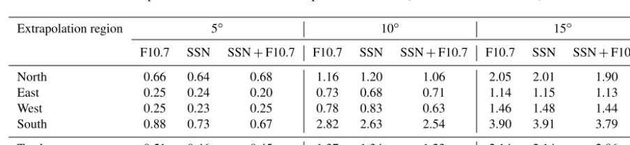
Table 4.One-month mean of extrapolation RMS errors with three parameterizations (NN model, unit=TECU).

Extrapolation region 5◦ 10◦ 15◦

F10.7 SSN SSN+F10.7 F10.7 SSN SSN+F10.7 F10.7 SSN SSN+F10.7

North 0.66 0.64 0.68 1.16 1.20 1.06 2.05 2.01 1.90 East 0.25 0.24 0.20 0.73 0.68 0.71 1.14 1.15 1.13 West 0.25 0.23 0.25 0.78 0.83 0.63 1.46 1.48 1.44 South 0.88 0.73 0.67 2.82 2.63 2.54 3.90 3.91 3.79

Total 0.51 0.46 0.45 1.37 1.34 1.23 2.14 2.14 2.06

The difference may mainly result from the fact that the generalization performance of the SVM model is better than that of the NN for the ionospheric variations. Since iono-sphere environment depends on its geomagnetic locations, the proposed extrapolation algorithm performance might be different at other locations. If the estimation region is changed, a new training and optimization process should be performed.

In order to determine optimal parameters between F10.7 and SSN, two more cases are tested; F10.7 only and SSN only. Optimal estimator structure is changing with the selec-tion of input parameters. Before comparing the single param-eter (F10.7 only or SNN only) results with the dual paramparam-eter (F10.7 and SNN) results, the same types of parameter opti-mizations are performed as those in Figs. 5 and 6 for each single parameter case. The SVM C value is set to 10 000 for both cases. The optimal numbers of hidden neurons are se-lected to 55 for the F10.7 case and 45 for the SSN case.

The extrapolation RMS errors of the single (F10.7 or SSN) and dual (F10.7+SSN) parameters are presented in Table 3 (SVM) and Table 4 (NN). The total mean errors of the single parameter cases are greater than the dual parameter case at all extrapolation points for both estimation models. Increase of the NN errors with the single parameters at north and south points are significant. Effect of F10.7 and SSN may be complementary to each other during geomagnetic storm days (19–22 October). In this period, the estimation error re-duction by the dual parameters are 26 % for SVM model and 22 % for NN model.

6 Conclusions

environ-mental parameters are used as input data sets to train the SVM algorithm. From the training results, 1 month of iono-spheric delay data outside the input data region is estimated. In addition to solar and geomagnetic environmental param-eters, current ionospheric delay data in the inner data region are used to estimate the ionospheric delay data in the outside region.

The estimation accuracy is evaluated at 12 points; four di-rections (north, south, east, and west) and three distances (5, 10, and 15◦). The accuracy improvement by the SVM is com-pared with the NN. The 1-month mean of the estimation er-ror produced by the SVM is 0.33 TECU for the 5◦region, 1.01 TECU for the 10◦ region, and 1.95 TECU for the 15◦ region. The improvement levels over the NN for the 5, 10, and 15◦regions are 26.7, 17.9, and 5.3 %, respectively. The error reduction by the SVM over NN is more significant at near points than at remote points.

Among the four directions, the error in the south region is the largest. The ionospheric delay and variation in the north region is usually smaller than the delay either in the east or west, but the extrapolation accuracy in the north region is even larger than in the east or west. A larger spatial gradient along the south–north direction over the east–west direction may explain this difference. This dependency on the iono-spheric spatial gradient can be explained by the inherent na-ture of extrapolation. A large gradient along the south–north direction implies more sensitivity along the south–north di-rection data. The north point data are more sensitive to the southern region’s input data than the western or eastern re-gions’ input data. Since the southern region’s input data has a larger variation than other regions, its variation directly af-fects the north point estimate and increases the error.

Although artificial neural networks are the most widely used machine learning algorithm for classification and re-gression problems, a SVM model is also powerful for pre-dicting problems because of its generalization performance. Because a SVM is defined by a convex optimization prob-lem, there are no local minima solutions. As SVM is based on structural risk minimization, it shows excellent general-ization performance. In the case of our ionosphere extrapo-lation problem, the SVM demonstrates a better performance than the NN.

Data availability. The IGS global ionosphere map data are avail-able in the IGS data center. Ionosphere map data used in the analy-sis can be freely accessed at ftp://cddis.nasa.gov/pub/gps/products/ ionex/ (IGS, 2019).

Competing interests. The authors declare that they have no conflict of interest.

Acknowledgements. This research was supported by the Space Core Technology Development Program funded by the Ministry of Science and Information and Communications Technology (ICT) (NRF-2016M1A3A3A02016943).

Edited by: Dalia Buresova

Reviewed by: three anonymous referees

References

Akhoondzadeh, M.: Support vector machines for TEC seismo-ionospheric anomalies detection, Ann. Geophys., 31, 173–186, https://doi.org/10.5194/angeo-31-173-2013, 2013.

Ban, P. P., Sun, S. J., Chen, C., and Zhao, Z. W.: Fore-casting of low-latitude storm-time ionospheric f0F2

using support vector machine, Radio Sci., 46, 1–9, https://doi.org/10.1029/2010RS004633, 2011.

Borovsky, J. E. and Denton, M. H.: Differences between CME-driven storms and CIR-CME-driven storms, J. Geophys. Res., 111, A07S08, https://doi.org/10.1029/2005JA011447, 2006. Chen, C., Wu, Z. S., Ban, P. P., Sun, S. J., Xu, Z. W., and

Zhao, Z. W.: Diurnal specification of the ionospheric f0F2

pa-rameter using a support vector machine, Radio Sci., 45, 1–13, https://doi.org/10.1029/2010RS004393, 2010.

Cristianini, N.: Support vector and kernel machines, Tutorial at the 18th Int. Conf. Mach. Learn., 2001.

Denton, M. H., Borovsky, J. E., Skoug, R. M., Thomsen, M. F., Lavraud, B., Henderson, M. G., McPherron, R. L., Zhang, J. C., and Liemohn, M. W.: Geomagnetic storm driven by ICME-and CIR-dominated solar wind, J.Geophys.Res., 111, A07S07, https://doi.org/10.1029/2005JA011436, 2006.

Ferris, M. C. and Munson, T. S.: Interior-point methods for mas-sive support vector machines, SIAM J. Optim., 13, 783–804, https://doi.org/10.1137/S1052623400374379, 2004.

Gunn, S. R.: Support vector machines for classification and regres-sion, ISIS Technical Report, 14, 1998.

Habarulema, J. B., McKinnell, L. A., and Opperman, B. D. L.: Re-gional GPS TEC modeling; Attempted spatial and temporal ex-trapolation of TEC using neural networks, J. Geophys. Res., 116, 1–14, https://doi.org/10.1029/2010JA016269, 2011.

Huang, W., Nakamori, Y., and Wang, S. Y.: Forecasting stock market movement direction with support vec-tor machine, Comput. Operat. Res., 32, 2513–2522, https://doi.org/10.1016/j.cor.2004.03.016, 2015.

Huang, Z. and Yuan, H.: Ionospheric single-station TEC short-term forecast using RBF neural network, Radio Sci., 49, 283–292, https://doi.org/10.1002/2013RS005247, 2014.

International GNSS Service (IGS): Global Ionosphere Map Data Archive, available at: ftp://cddis.nasa.gov/pub/gps/products/ ionex/, last access: 28 January 2019.

Jayapal, V. and Zain, A. F. M.: Interpolation and extrapolation tech-niques based neural network in estimating the missing iono-spheric TEC data, in: Progress in Electromagnetic Research Symposium (PIERS), 695–699, 2016.

Kim, J. and Kim, M.: Extending ionospheric correction coverage area by using extrapolation methods, J. Kor. Soci. Aeros. Sci. Fli. Operat., 22, 74–81, https://doi.org/10.12985/ksaa.2014.22.3.074, 2014.

Kim, J., Lee, S. W., and Lee, H. K.: An annual variation analysis of the ionospheric spatial gradient over a regional area for GNSS applications, Adv. Spa. Res., 54, 333–341, https://doi.org/10.1016/j.asr.2014.03.024, 2014.

Kim, M. and Kim, J.: Extending ionospheric correction coverage area by using a neural network method, Int. J. Aero. Spa. Sci., 17, 64–72, https://doi.org/10.5139/IJASS.2016.17.1.64, 2016. Kumluca, A., Tulunay, E., and Topalli, I.: Temporal and

spatial forecasting of ionospheric critical frequency using neural networks, Radio Sci., 34, 1497–1506, https://doi.org/10.1029/1999RS900070, 1999.

Leandro, R. F. and Santos, M. C.: A neural network approach for re-gional vertical total electron content modelling, Stud. Geophys. Geod., 51, 279–292, https://doi.org/10.1007/s11200-007-0015-6, 2006.

Mansoori, A. A., Khan, P. A., Bhardwaj, S., Atulkar, R., and Purohit, P. K.: Ionospheric irregularity influences on GPS time delay, Russian J. Earth Sci., 15, 1–9, https://doi.org/10.2205/2015ES000555, 2015.

McKinnell, L. A. and Friedrich, M.: A neural network-based iono-spheric model for the auroral zone, J. Atmos. Sol.-Terr. Phy., 69, 1459–1470, https://doi.org/10.1016/j.jastp.2007.05.003, 2007. Mohandes, M. A., Halawani, T. O., Rehman, S., and

Hussain, A.: Support vector machines for wind speed prediction, Renewable Ener., 29, 939–947, https://doi.org/10.1016/j.renene.2003.11.009, 2014.

Okoh, D., Owolabi, O., Ekechukwu, C., Folarin, O., Arhiwo, G., Agbo, J., Bolaji, S., and Rabiu, B.: A regional GNSS-VTEC model over Nigeria using neural net-works: A novel approach, Geode. Geodyn., 7, 19–31, https://doi.org/10.1016/j.geog.2016.03.003, 2016.

Razin, M. R. G. and Voosoghi, B.: Wavelet neural networks using particle swarm optimization training in modeling regional iono-spheric total electron content, J. Atmos. Sol.-Terr. Phy. 149, 21– 30, https://doi.org/10.1016/j.jastp.2016.09.005, 2016.

Song, R., Zhang, X., Zhou, C., Liu, J., and He, J.: Pre-dicting TEC in China based on the neural networks opti-mized by genetic algorithm, Adv. Space Res., 62, 745–759, https://doi.org/10.1016/j.asr.2018.03.043, 2018.

Vukovi´c, J. and Kos, T.: Ionospheric spatial and tempo-ral gradients for disturbance characterization, Proceeding of 2016 European Navigation Conference (ENC), Helsinki, 1–4, https://doi.org/10.1109/EURONAV.2016.7530564, 2016. Wielgosz, P., Grejner-Brzezinska, D., and Kashani, I.: Regional

ionosphere mapping with kriging and multiquadric methods, J. GPS., 2, 48–55, https://doi.org/10.5081/jgps.2.1.48, 2003. Wu, Y. W., Liu, R. Y., Zhang, B. C., Wu, Z. S., Ping, J. S., Liu,