An enhanced forest classification scheme for modeling vegetation–climate interactions based on national forest inventory data

https://doi.org/10.5194/bg-15-399-2018

© Author(s) 2018. This work is distributed under the Creative Commons Attribution 4.0 License.

An enhanced forest classification scheme for modeling

vegetation–climate interactions based on national

forest inventory data

Titta Majasalmi1, Stephanie Eisner1, Rasmus Astrup1, Jonas Fridman2, and Ryan M. Bright1

1_{Norwegian Institute of Bioeconomy Research (NIBIO), Department of Forest and Climate, 1431 Ås, Norway} 2_{Swedish University of Agricultural Sciences (SLU), 901 83 Umeå, Sweden}

Correspondence:Titta Majasalmi (titta.majasalmi@nibio.no) Received: 14 July 2017 – Discussion started: 9 August 2017

Revised: 29 November 2017 – Accepted: 1 December 2017 – Published: 18 January 2018

Abstract.Forest management affects the distribution of tree species and the age class of a forest, shaping its overall struc-ture and functioning and in turn the surface–atmosphere ex-changes of mass, energy, and momentum. In order to at-tribute climate effects to anthropogenic activities like for-est management, good accounts of forfor-est structure are nec-essary. Here, using Fennoscandia as a case study, we make use of Fennoscandic National Forest Inventory (NFI) data to systematically classify forest cover into groups of simi-lar aboveground forest structure. An enhanced forest classi-fication scheme and related lookup table (LUT) of key for-est structural attributes (i.e., maximum growing season leaf area index (LAImax), basal-area-weighted mean tree height, tree crown length, and total stem volume) was developed, and the classification was applied for multisource NFI (MS-NFI) maps from Norway, Sweden, and Finland. To pro-vide a complete surface representation, our product was in-tegrated with the European Space Agency Climate Change Initiative Land Cover (ESA CCI LC) map of present day land cover (v.2.0.7). Comparison of the ESA LC and our enhanced LC products (https://doi.org/10.21350/7zZEy5w3) showed that forest extent notably (κ=0.55, accuracy 0.64) differed between the two products. To demonstrate the poten-tial of our enhanced LC product to improve the description of the maximum growing season LAI (LAImax)of managed forests in Fennoscandia, we compared our LAImaxmap with reference LAImax maps created using the ESA LC product (and related cross-walking table) and PFT-dependent LAImax values used in three leading land models. Comparison of the LAImax maps showed that our product provides a spatially more realistic description of LAImaxin managed

Fennoscan-dian forests compared to reference maps. This study presents an approach to account for the transient nature of forest struc-tural attributes due to human intervention in different land models.

1 Introduction

LC class is further divided into a number of subclasses ac-cording to their biophysical properties, grouping them into what is often termed plant functional types (PFTs) or “broad groupings of plant species that share similar characteristics (e.g., growth form) and roles (e.g., photosynthetic pathway) in ecosystem function” (Wullschleger et al., 2014). LC maps are converted into PFT maps using various model-dependent algorithms (e.g., Lawrence and Chase, 2007; Reick et al., 2013) or “cross-walking” tables (e.g., ESA LC, 2017, manual p. 75; Poulter et al., 2015).

Differences in forest structure within a given LC type (or PFT) can differ substantially (Kuuluvainen et al., 2012; New-ton, 1997), and preserving within-LC (or within-PFT) differ-ences in forest structure is necessary for more accurate mod-eling of surface fluxes in forests. While some land models assimilate local information on present day forest structure from satellite remote sensing to account for within-PFT vari-ation (e.g., Community Land Model 4.5, CLM4.5, Oleson et al., 2013; Jena Scheme of Atmosphere Biosphere Coupling in Hamburg, JSBACH, Reick, 2012), future structure must still be prescribed. Because land use transitions in model-ing simulation studies of anthropogenic LC change are often represented by a change in PFT area in land models, post-disturbance changes to structure within forest PFTs go unde-tected (Lawrence et al., 2012; Reick et al., 2013). Hence, a forest classification that accounts for major variation in key structural attributes, such as LAI or canopy height, may lead to better predictions of surface fluxes in forests, not only in studies of prescribed land cover and/or management change, but also for dynamic vegetation studies that rely on fixed PFT parameters obtained from lookup tables (LUTs). The time-invariant nature of the fixed parameter LUTs may be avoided by increasing the number of forest classes within a single forest PFT with sufficient differentiation in key struc-tural attributes (i.e., from young to mature forests). In addi-tion to grouping forests according to their shared phenologi-cal characteristics, further grouping according to their struc-tural characteristics (i.e., accounting for the effects of forest management) would strengthen prediction confidence in in-tensively managed regions.

LC data needed by land models should ideally be represen-tative of sufficiently large areas because incorporating frag-mented data stemming from individual research sites and in-dividual research experiments is limited by available com-puting resources and rapidly increasing model complexity. Most countries are currently conducting National Forest In-ventories (NFIs) to quantify the extent and amount of forest resources with standardized reporting for compiling global Forest Resources Assessments (FRAs; e.g., FAO, 2015). NFI data have previously been used in research aiming to attribute climate effects to management activities because they reflect the human influence on forest structure (Bright et al., 2014; Naudts et al., 2015, 2016). However, as NFI data character-ize only forested areas, other LC data are needed to form the complete surface representation required by land

mod-els. The state-of-the-art LC products, such as the European Space Agency (ESA) Climate Change Initiative (CCI) LC product (ESA LC, 2017), allow for cross-walking from LC classes to PFTs used in land models. It is noteworthy that ESA LC products have high spatial resolution (0.003◦) com-pared to the common global grid sizes (e.g., 0.5–1◦) used in land models, which allows for more flexibility in cross-walking and LC data aggregation.

In this study, we develop a forest classification scheme based on NFI data to better characterize the transient nature of forest key structural attributes to provide more realistic starting values for different land model simulations. We de-velop our concept using NFI data from Fennoscandia as it represents one of the most intensively managed forested re-gions of the world (e.g., Kuuluvainen et al., 2012). From the perspective of climate modeling, NFI data are well suited for enhancing the structural description of forests in global LC datasets because similar data are available for most devel-oped countries and new data are collected systematically. The aims of this study are to (1) develop a semi-objective clus-tering analysis approach to come up with an LC-dependent structural LUT, which reflects the transient nature of the key forest structural attributes in managed forests, (2) create a new forest LC product for Fennoscandia based on multi-source NFI (MS-NFI) data to allow for the spatial applica-tion of the LUT of key structural attributes, (3) augment the new forest classification by importing non-forest LC classes of the ESA LC product to form the complete surface rep-resentation required by land models, (4) compare the for-est extent of the new LC product with the original ESA LC product to point out geographic areas where the largest dif-ferences occur to provoke discussion on alternative informa-tion sources for parameterizing land models, and (5) visual-ize and compare maps of our maximum growing season LAI (LAImax)with reference LAImax maps produced using the ESA LC product, a model-generic cross-walking table (Poul-ter et al., 2015), and PFT-dependent LAImax values used in three land models: JSBACH, Joint UK Land Environment Simulator (JULES), and Organizing Carbon and Hydrology in Dynamic EcosystEms (ORCHIDEE).

2 Materials and methods 2.1 Data

2.1.1 NFI plot data

di-versity in forest structure throughout the Fennoscandian re-gion is well represented in the Swedish and Norwegian NFI data. The Norwegian NFI contained data from 10 813 circu-lar 8.92 m radius sample plots (250 m2), while the Swedish data were from 14 032 circular 10 m radius sample plots (314 m2). Plots that were divided (i.e., not completely cir-cular) or that did not have trees were excluded from the data prior to the analysis. The main tree species of the area are Norway spruce (Picea abies(L.) H. Karst.), Scots pine (Pinus sylvestris, L.), and silver and downy birches (Betula pendula Roth andpubescens Ehrh.). Monocultural plots of birch are rare, but birches are common in plots with different species mixtures. Plot data were classified as spruce-, pine-, or deciduous-dominated (contains also other tree species) forests based on species with the largest share of total stem volume (m3ha−1) on the sample plot (Table 1.).

2.1.2 MS-NFI data

NFI plot characteristics are extrapolated for areas between the NFI plots using the non-parametrick–nearest-neighbor (kNN) estimation method (e.g., Tomppo et al., 2014). The ex-trapolation step is called multisource NFI (MS-NFI) because it employs data from different remote sensing systems (i.e., satellite and aerial platforms) and NFI plots. MS-NFI applies high-spatial-resolution (< 900 m2)satellite images to sepa-rate forested areas from other LC classes and digital terrain models to correct topographical distortions. In Fennoscan-dia, the common stand size is only 1–2 ha (i.e., landscape is fragmented by forests with different development stages) and thus high-spatial-resolution satellite products are needed to prepare the MS-NFI maps. All processing of the MS-NFI data is done by forest authorities. MS-NFI maps are typi-cally provided for forest variables such as Lorey’s height (i.e., basal-area-weighted mean tree height) (H, m), forest stand age (years), and stem volume (V, m3ha−1) by species. The newest MS-NFI maps for Finland (of 2013) and Swe-den (of 2010) were downloaded from the Natural Resources Institute Finland (LUKE) portal (LUKE, 2016) and from the Swedish University of Agricultural Sciences (SLU) por-tal (SLU, 2016). For Norway, MS-NFI data (compiled dur-ing the first decade of the twenty-first century) called “SAT-SKOG” (Gjertsen, 2007, 2009) and a forest resource map called “AR5” (Ahlstrøm et al., 2014) were used to obtain all required inputs and coverage of the northernmost forest areas (i.e., Finnmark county; Supplement S1).

2.1.3 ESA LC product

The ESA LC-product series contains a set of annual maps from 1992 to 2015 (ESA LC, 2017). The product series fol-lows processing in which a baseline LC product is applied; although the annual maps are not fully independent from each other, they are temporally consistent. The baseline LC product was based on MERIS FR and RR archive between

the years 2003 and 2012 and was back-dated and updated based on data from other satellite sensors (AVHRR between 1992 and 1999, SPOT-VGT between 1999 and 2013, and PROBA-V between 2013 and 2015). In this study, the newest 2015 (v.2.0.7) LC product was used as it is more likely to be used by land modelers. This LC-product version has been validated against GlobCover 2009 reference data (cf. p. 39 in the product manual ESA LC, 2017). The spatial resolution of the ESA LC product is∼0.003◦, and it follows standardized hierarchical classification by the United Nations Land Cover Classification System (UN-LCCS), which allows for the con-version of LC classes into PFTs based on a cross-walking table (ESA LC, 2017, manual p. 75; Poulter et al., 2015). The 2015 ESA LC product contains three LC classes to de-scribe forests in Fennoscandia: broadleaved deciduous (60– 62), needleleaved evergreen (70–72), and mixed broadleaved and needleleaved (90; ESA LC labels in parentheses). The second label digit from the left is designed to indicate for-est fraction within an LC pixel: the canopy is “closed” when the forest pixel cover fraction is > 40 % (labels 61 and 71) and “open” when the forest pixel cover fraction is between 15 and 40 % (labels 62 and 72). Labels 60 and 70 are used to indicate that the within-pixel forest fraction is more than 15 %, but it is not known whether that pixel is closed or open. The 2015 ESA LC product for Fennoscandia contained only classes 60, 61, 70, and 90 (i.e., no pixels were assigned to subclasses 62, 71, or 72).

2.2 Methods

2.2.1 Forest classification scheme

NFI data were first used to develop the forest classification scheme based on four key forest structural attributes: total stem volume (V), Lorey’s height (H), crown length (CL), and LAImax (LAImax calculation is described in Supple-ment S2; Fig. 1). V defines species dominance, H corre-sponds with the aerodynamic height or ztop (Nakai et al., 2010), CL is needed to estimate canopy bottom height or

zbottom(i.e.,zbottom=H – CL; modeling of CL described in

Supplement S3), and LAImaxquantifies the exchange surface area between the land surface and the atmosphere. First, a clustering analysis of the NFI data was used to find medoids of the four-dimensional (4-D)V–H–CL–LAImaxclusters be-cause forest variables are not independent from each other. After defining the 4-D cluster centers, another Euclidean-distance-based classifier was used to define the 4-D cluster boundaries in order to apply the classification on MS-NFI data. An overview of the analysis is shown in Fig. 1.

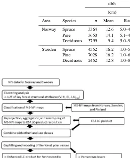
Table 1.Descriptive statistics for the National Forest Inventory (NFI) data. Abbreviations:nis the number of sample plots, dbh is diameter at breast height,H is basal-area-weighted mean tree height (i.e., Lorey’s height), andV is total stem volume.

dbh H V

(cm) (m) (m3ha−1)

Area Species n Mean Range Mean Range Mean Range

Norway Spruce 3364 12.6 5.0–49.0 13.0 2.9–32.3 152.0 0.2–1492.4 Pine 3650 14.1 5.1–48.9 11.5 2.4–28.6 97.8 0.2–656.6 Deciduous 3799 9.4 5.0–99.9 8.3 2.4–24.8 53.0 0.2–592.9

Sweden Spruce 4552 16.2 1.0–52.0 15.3 1.4–40.2 177.8 0.5–1010.2 Pine 7028 16.2 1.0–64.6 13.6 1.4–32.1 120.0 0.6–752.3 Deciduous 2452 12.8 1.0–81.2 12.8 1.5–32.6 101.9 0.4–1001.5

Figure 1. Flowchart for developing and applying the forest clas-sification scheme (Sects. 2.2.1 and 2.2.2). Abbreviations: Na-tional Forest Inventory (NFI), lookup table (LUT), total stem vol-ume (m3ha−1) (V), Lorey’s height (H), crown length (CL), max-imum growing season leaf area index (LAImax), multisource NFI (MS-NFI; i.e., products provided by forest authorities), European Space Agency Land Cover (ESA LC) product.

plotting the curve between the total within-cluster sum of squares (wcss) and the number of clusters (k) and then ob-serving around which k the relationship resembles a “bent knee” (i.e., the “elbow method”; Ketchen Jr. and Shook, 1996). Analysis was run using the R package “factoextra” (Kassambara and Mundt, 2017). In each species group the bent knee was located betweenk=3 andk=5, and thus the optimal k was set to 4 (i.e., the number of structural sub-groups was set to four). Then, using the predefined number of structural subgroups (k=4) within each species group (n=3), ak-medoids clustering analysis was used to define the cluster “centroids” (i.e., medians) within theV–H–CL– LAImax space to form a LUT of the key forest structural attributes (n×k=12 forest classes). The k-medoids algo-rithm is a data partitioning method in which each cluster is represented by one of the cluster objects (i.e., all subgroup

LUT values (V,H, CL, and LAImax)are from the same plot; Kaufman and Rousseeuw, 1990). Thek-medoids algorithm assigns all plots to the nearest cluster centers and calculates the wcss. New cluster centers are updated and the plots are reassigned. Cluster centers are adjusted iteratively until they do not change. Thek-medoids algorithm was chosen because only the number of clusters is required as an input and also because it is robust against outliers. The analysis was run us-ing the “cluster” package in R (Maechler, 2017).

A method to assess cluster boundaries was needed because many plots were located near the edges of the 4-D clusters. We chose to determine cluster boundaries using V and H

since these are often available for large geographical areas from MS-NFIs. Mahalanobis (1936) distance (MD) was used to quantify the within-cluster variation in theV andHspace (i.e.,V–H space) because it corresponds to the Euclidean distance afterV andHhave been normalized. MD is a mul-tidimensional method to determine how many standard de-viations a data point is away from the class mean. For MD calculation the cluster mean values were obtained based on the 4-D (i.e.,V,H, CL, and LAImax)and not in 2-D (i.e.,V andH) clusters, and thus the cluster boundaries are not cir-cular. MD values were calculated for each species group and the respective subgroups. The binning (i.e., grid of 14×14) interval of theV–H space was set subjectively to add reso-lution on younger forest structures. For each grid cell and for each subgroup, a median MD value was calculated. To rep-resent results using a grid surface, the cell was assigned to a subgroup with the smallest median MD.

2.2.2 Compiling the enhanced LC product

spruce was assigned to the deciduous group. After the species group was assigned, a griddedV–Hspace was used to deter-mine pixel subgroup. Possible V–H combinations without MD value (i.e., falling outside theV–Hspace) were assigned to the closest subgroup based onV. After classifying all data, the forest classes were recoded as integers between 1 and 12 (i.e., three species groups×four structural subgroups).

The classified MS-NFI maps were reprojected, aggre-gated, and resampled to complement the ESA LC product (v.2.0.7; ESA LC, 2017) to form the complete surface repre-sentation required by land models. Two types of aggregation routines were used for upscaling: forest class was assigned based on mode (among the 12 forest classes) and within-pixel forest cover fraction based on mean (for this purpose, forested pixels in MS-NFI data were recoded as 100 and other pixels as 0). In other words, for each forested ESA LC pixel (∼90 000 m2), forest class and within-pixel forest cover fraction (%) were obtained based on classified MS-NFI maps (∼260 or ∼630 m2). Two exceptions occurred: (1) if the ESA LC pixel was not classified as forest but the MS-NFI maps indicated the presence of forest, and (2) if the ESA LC pixel was classified as a forest but MS-NFI maps indicated non-forest. For pixels that were classified as forest by the ESA LC product but the forest cover fraction within that pixel in the enhanced LC product did not exceed the 15 % threshold (i.e., definition used by the ESA LC prod-uct) according to the MS-NFI data, forest class was assigned based on moving average interpolation (referred to as “gap-filling”). Gapfilling was necessary because land (climate) models require completeness in LC to resolve computations of mass, energy, and momentum fluxes (note: gapfilled pix-els are coded separately, which allows them to be either in-cluded in or exin-cluded from analysis). Non-forest LC classes were imported from the ESA LC product to supplement our forest pixels.

To allow for more flexible cross-walking or aggregation to a lower spatial resolution in the preparation of surface datasets in land models, for each forest LC pixel, coverage fractions (referred to as “percentage layers”) for each of the 12 forest classes were calculated (i.e., 12 layers with values ranging between 0 and 100 based on subgroup abundance within the ESA LC pixel). In addition, gapfilled pixels and non-forest LC classes are provided as own layers. These lay-ers also allow more flexibility for modellay-ers in choosing the number of desired input land cover classes (i.e., modelers may use, for example, the three most abundant forest classes instead of keeping to the most abundant one). Raster analyses were performed using the “rgdal” (Bivand et al., 2017) and “raster” (Hijmans, 2017) packages in R. The enhanced LC product for Fennoscandia, including the percentage layers, can be downloaded from Majasalmi et al. (2017).

2.2.3 Comparison of the LC products

To highlight areas where the forest extent differed the most, a difference map between the enhanced “back-classified” (i.e., into ESA LC classes) map and ESA LC product was calcu-lated using∼0.3◦resolution. This resolution was chosen as it represents a good compromise between higher-resolution regional modeling (0.05–0.1◦) and coarser-resolution re-gional and global modeling (0.5–1◦). In addition, LC-class changes (e.g., from cropland to conifer forest) were quanti-fied using a confusion matrix between the ESA LC classes and enhanced back-classified map classes in the original product resolution (∼0.003◦). The back-classification was done using the percentage layers of different forest sub-groups: if >=70 % of the MS-NFI pixels within the ESA LC pixel were classified into the conifer or deciduous group, the pixel was classified as “needleleaved” (class 70) or “broadleaved” (class 60), but otherwise it was classified as “mixed” (class 90). The difference map was calculated after both products (i.e., the enhanced back-classified map and the ESA LC product) were aggregated to∼0.3◦resolution us-ing pixel modes. The LC class changes are presented with a confusion matrix between the ESA LC product and the enhanced back-classified map; each row of the matrix rep-resents an occurrence in the enhanced back-classified map, while each column represents the respective occurrence in the ESA LC product. The percentage of pixels belonging to the same LC class in both products is shown in diagonal, whereas percentage values outside the diagonal quantify the change (“confusion”) between the different LC classes. The confusion matrix was calculated using the “caret” package (Kuhn, 2008) in R.

2.2.4 Comparison of LAImaxmaps

To demonstrate the potential of our LC product to provide more realistic LC-dependent values of key forest structural attributes for forested areas in Fennoscandia, we compared our LAImaxmap (i.e., produced using enhanced LC product and related LUT) with reference LAImaxmaps produced us-ing the ESA LC product, a model-generic cross-walkus-ing ta-ble (Poulter et al., 2015), and PFT-dependent LAImaxvalues used in ORCHIDEE, JULES, and JSBACH. Only forested pixels were used for demonstration.

Figure 2.Gridded representation of vegetation subgroups, i.e.,(a)spruce,(b)pine, and(c)deciduous, within the total stem volume (V) and Lorey’s height (H) space (referred to asV–H space) based on NFI data. Visualization is required to map subgroup distribution inV–H space and is used to apply the classification to the MS-NFI maps.

Table 2.A forest classification scheme lookup table (LUT). Abbreviations:V is total stem volume (m3ha−1),His Lorey’s height (m), CL is crown length (m), and LAImaxis maximum growing season leaf area index (m2m−2). The “Recoded label” column is a key to be used with the enhanced CL product. Interquartile range (i.e., first quartile subtracted from the third quartile) is given inside parentheses.

Species group Subgroup Recoded label V H CL LAImax

Spruce 1 301 22 (28.9) 7.5 (3.1) 6.3 (2.8) 1.4 (1.6)

2 302 92.2 (51.7) 12.3 (2.5) 10.1 (2.2) 4.3 (2.2) 3 303 201.3 (70.1) 16.8 (3.1) 13.2 (2.6) 6.7 (2.5) 4 304 373.9 (138.9) 22 (4.5) 15.8 (3.5) 9.1 (3.4)

Pine 1 305 20.8 (23.1) 7.5 (2.8) 4.6 (1.7) 0.9 (1)

2 306 80 (49.2) 11.6 (2.4) 6.7 (1.4) 2.4 (1.4) 3 307 129.5 (67.9) 17 (3.9) 9.4 (2) 2.3 (1.2) 4 308 236.4 (107.1) 17.2 (5) 8.4 (1.6) 4.4 (1.5)

Deciduous 1 309 7.2 (10.8) 4.9 (1.6) 3.2 (1.1) 0.5 (0.7) 2 310 36.1 (28.9) 8.4 (2.1) 5.5 (1.3) 1.8 (1.6) 3 311 97.6 (50.8) 12.2 (3.7) 7.9 (2.5) 3.9 (2.1) 4 312 227 (111.2) 18.3 (5.5) 10.3 (3.2) 7 (3.2)

were obtained as an average of BDT and NET values because all the required input data (e.g., values for needleleaf decid-uous tree (NDT) and BES) were not available to follow the ESA LC-product cross-walking scheme.

JULES, JSBACH, and ORCHIDEE LUTs employ PFT-dependent LAImax values. In JULES according to Clark et al. (2011), the PFT-dependent LAImax values are 9 for a broadleaf tree (BDT), 5 for a needleleaf tree (NET), 4 for a C3grass (natural grass), and 3 for a shrub (BDS; acronyms used by the ESA LC cross-walking table in parenthesis). In ORCHIDEE as reported by Lathière et al. (2006), the respec-tive PFT-dependent LAImax values are 4.5 for both boreal BDT and NET, and 2.5 for a C3 grass (same LAImax also used for BDS). In JSBACH according to Schürmann et al. (2016), the PFT-dependent LAImax value was 5 for extrat-ropical deciduous trees (BDTs), 1.7 for coniferous evergreen

trees (NETs), and 3 for C3grass (same LAImaxalso used for BDS).

3 Results

3.1 Forest classification scheme

Table 3.The percentage (%) of forest pixels (i.e., excluding gapfilled pixels) belonging to different species groups in the enhanced LC product (referred to as Fennoscandia) and separately for each country (the spatial distribution of different forest subgroups and their frequency distributions are shown in Fig. 3). Values are based on MS-NFI data.

Fennoscandia (%) Norway (%) Sweden (%) Finland (%)

Spruce 22.9 28.9 29.0 13.7

Pine 58.1 28.9 58.3 71.7

Deciduous 19.0 42.3 12.6 14.6

may haveV up to 1500 m3ha−1. In pine-dominated plots the

V did not exceed 900 m3ha−1, and in deciduous plots the highestV was 1100 m3ha−1. In spruce-dominated plots, the

H exceeded 30 m with many differentVs, whereas for pine the 30 m was exceeded either when the respectiveV was less than 50 m3ha−1(i.e., the tree is left for seed production dur-ing harvestdur-ing, which is a common forest regeneration strat-egy in Fennoscandia) or large (more than 500 m3ha−1). In plots dominated by deciduous species the 30 m is exceeded after V was more than 150 m3ha−1. The location and size (i.e., patterns) of different subgroups inV–H space cannot be directly compared between different species groups, as Euclidean distances were used for their classification.

3.2 Enhanced LC product

The majority (58 %) of the forest pixels in Fennoscan-dia were classified as pine dominated, which was also the largest species group in Sweden (58 %) and in Finland (72 %; Table 3). However, in Norway the largest species group was deciduous broadleaf (42 %). Finland had a slightly higher percentage of deciduous forests than Sweden. Spruce-dominated forest was the smallest species group in Finland (14 %). Visual assessment of the spatial distribution of dif-ferent species groups and their subgroups showed that low-land areas in Finlow-land and in Sweden were mainly dominated by pines and spruces, whereas deciduous species were most abundant in the northernmost, mountainous, and coastal ar-eas (Fig. 3). In Fennoscandia the most abundant subgroup within spruce-dominated forest was “Spruce 3” (i.e., species group “spruce” and subgroup number “3”) with class me-dian values of V =201 m3ha−1 _{and H=17 m (see} Ta-ble 2). Within the pine-dominated forest the most abundant subgroup was “Pine 2” with class median V =80 m3ha−1 and H=12 m. For the deciduous species group the me-dian values of the largest subgroup “Deciduous 1” were

V =7 m3ha−1andH=5 m.

3.3 Forest extent comparison

In order to assess agreement between the two LC prod-ucts, the enhanced LC product was back-classified into ESA LC classes using the percentage layers of different forest subgroups. The kappa coefficient (measure of agreement

Figure 3.Spatial distribution of MS-NFI forest classes (i.e., with-out gapfilled forest pixels) in Fennoscandia. The first part of thex label is the species group and the number refers to the respective subgroup number (see Fig. 2.). The forest subgroup was assigned based on the most abundant forest class within the ESA LC pixel. For colors, see the online version of the article.

T able 4. Confusion matrix in percentage (%) between the ESA LC product and the enhanced back-classified LC product. Bold font is us ed to indicate the 10 classes with the highest percentage of pix els. Small percentages are sho wn as 0.00. The kappa coef fic ient w as 0.55. Label definitions are sho wn in Fig. 4. In order to compare the tw o LC products the enhanced LC product w as back-classified into ESA LC classes. Column names are the ESA LC-class labels and column sums represent the fraction of that LC class present in the ESA LC product. The ro w sums represent the fraction of that LC class present in the enhanced back-classified map. The percentage of pix els belonging to the same LC class in both products is sho wn in diagonal (e.g., the fraction of pix els classified into LC class 70 is 30.3 %). Percentage v alues outside the diagonal describe the change (“confusion”) between dif ferent LC classes (e.g., 14.4 % of pix els classified into LC cla ss 70 by the ESA LC product were classified into LC class 90 in the enhanced back-classified map). ESA 2015 LC product (v .2.0.7) 0 10 11 30 40 60 70 80 90 100 110 120 122 130 140 150 152 160 180 190 200 201 210 220 Sum: 0 10 2.5 2.5 11 0.3 0.3 30 0.2 0.2

Enhanced back-classified land cover classification

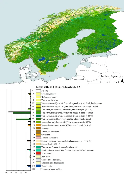
Figure 4.Enhanced back-classified map for Fennoscandia. The per-centage layers of forest subgroups were used to back-classify the data into ESA LC product classes (see Sect. 2.2.2.). Histograms show LC-class percentages for the enhanced back-classified map (lower bars with colors) and for the ESA LC product (black upper bars). For colors, see the online version of the article.

more forest classified pixels than the ESA LC product (note: the fraction of gapfilled forest pixels was 4.5 %). Forest area increased by 4.8 % at the expense of the ESA LC class shrub or herbaceous cover (class 180), 4.1 % at the expense of the LC class mosaic tree and shrub (> 50 %; class 100), 2.3 % at the expense of the LC class croplands (class 10), and 1.9 % at the expense of the LC class water bodies (class 210). The classified land area increased by 0.5 % as areas classified as “no data” in the ESA LC product were classified as forest in the enhanced LC product.

The spatial distribution of different LC classes and the class frequencies of the enhanced back-classified map are shown in Fig. 4, which shows both ESA LC-class labels and descriptions (note: ESA LC-product class frequencies are also shown for reference). The difference map of forest cover between the enhanced back-classified LC product and the ESA LC product pointed out that the areal representation of forests differs the most in mountainous areas in Norway

Figure 5.Difference in forest extent between the enhanced back-classified map and the ESA LC product. Both types of data were aggregated to∼0.3◦ resolution using mode to display the main differences in the two classifications spatially. The label “Gapfilled forest” is used to indicate areas that were mainly classified as forest by the ESA LC product, but the MS-NFI data indicated non-forest. Other labels (see Fig. 4.) show which main ESA LC classes were classified as forest in the enhanced back-classified map. Note that the confusion matrix between the ESA LC product and enhanced back-classified map was prepared using∼0.003◦ resolution (Ta-ble 4), whereas the map resolution shown here is∼0.3◦. For colors, see the online version of the article.

and Sweden, south and north Finland, and in middle to south Sweden in the area between Stockholm and lakes Vättern and Vänern (lakes visible in Fig. 4.; Fig. 5.). The areas classified as forest by the ESA LC product but not by MS-NFI data (“gapfilled forest” in Fig. 5.) were mainly located in moun-tainous areas in Norway and Sweden.

3.4 LAImaxmap comparison

values applied in JULES (mean LAImax=4.9, SD=0.9). It is noteworthy that the use of JSBACH and JULES PFT-dependent LAImaxvalues produced unnaturally high LAImax values for the northernmost areas dominated by deciduous species.

4 Discussion

This paper is a response to the “call to action” raised in the review by Ellison et al. (2017), which highlighted an urgent need to integrate forest effects on energy balances, hydrol-ogy, and climate into policy actions regarding climate change adaptation and mitigation. One of goals of this paper is to foster interdisciplinary discussions on alternative informa-tion sources, such as the existing NFI data, to enhance the representation of forest structures in different land modeling frameworks. Although NFIs from different countries have been shaped by local information needs, the work done by the Food and Agriculture Organization (FAO) in conducting global FRAs since 1948 has aided in developing national forest reporting standards. Currently, new assessments are carried out every 5 years and the 2015 assessment covered 93.5 % of the global forest area (Köhl et al., 2015). Thus, as the aim of an FRA is to describe the state and change of the world’s forests and keep policy makers informed, the same data could potentially be used to describe the current state of forests in land models. In this study, we developed a sim-ple clustering and classification scheme to allow for the re-iteration of our approach to NFI data from other countries. Classifying forests based on the structural properties they share at various successional stages under similar manage-ment conditions may be one way to link models of forestry with the land models employed in climate research. Impor-tant transient effects could then be included, for example through changes in area under a given successional stage, with forestry models providing the link to the time dimen-sion. Alternatively, distinct rule sets for successional dynam-ics following management disturbances could be developed analogous to those used to govern growth and competition in dynamic vegetation models (or land models run in dynamic vegetation mode).

Recently, other approaches have been developed for incor-porating forest management into existing land surface (cli-mate) models. For example, the radiative-transfer-based land surface model ORCHIDEE was parameterized to simulate the effects of forest management for biogeochemical and bio-physical variables (Naudts et al., 2015). The model was pa-rameterized using diameter-at-breast-height (dbh) data from different European NFIs (French, Spanish, Swedish, and German; i.e., the key input values were modeled based on dbh using allometric models), and 12 parameter sets for spe-cific tree species (instead of presenting groups of species such as PFTs) were presented. However, a major drawback of individual tree-based approaches is that existing global LC

Figure 6.Demonstration of how the enhanced LC product and the related LUT may be used to map local variations in important struc-tural attributes in forests, such as maximum growing season LAI (max LAI or LAImax). Maps of LAImaxin Fennoscandic forests using(a)our enhanced LC product and the related LUT,(b)ESA LC product and PFT-dependent LAImaxvalues used in JSBACH, (c)ESA LC product and PFT-dependent LAImax values used in ORCHIDEE, and(d)ESA LC product and PFT-dependent LAImax values used in JULES. For colors, see the online version of the arti-cle.

traits such as root traits cannot be measured using remote sensing.

At present, some countries, such as Finland and Sweden, have national airborne laser scanning (ALS) campaigns pro-ducing high-resolution forest structural data that could be used to obtain more accurate forest height estimates or to develop forest classification schemes for different land mod-els. However, the drawback of these ALS datasets is that they cannot be used to separate different tree species, which is one of the most important forest structural attributes. In addition, as few countries have national ALS datasets, the geographi-cal extent that could be covered using ALS-based forest clas-sification schemes remains limited. At present, the use of op-tical satellite data to classify forests is unquestionable due to their superior spatial and temporal resolution and will thus probably sustain their role as the most valuable tool for en-vironmental monitoring and mapping. While synthetic aper-ture radar (SAR) allows for more robust and temporally con-tinuous data collection compared to optical instruments (i.e., SAR is not limited to cloudless conditions unlike optical in-struments), the relatively low spatial resolution (km2)cannot be used to separate different aged forests in landscapes that are fragmented (into 0.01 km2units) by active forest manage-ment. Data from SAR could be used to harmonize MS-NFI data from different countries and to provide other land model inputs, such as soil moisture maps. In the future, approaches combining both optical and ALS–SAR data may be expected to become more common and thus allow for the develop-ment of more sophisticated forest classification schemes to increase the accuracy of climate predictions.

The forest extent differs significantly between the en-hanced LC product and the ESA LC product because they employ different forest definitions. The ESA LC product is based on series of satellite surface reflectance data (i.e., be-tween years 1992 and 2015) and the LC class is deduced based on pixel reflectance properties. However, processing the MS-NFI data employs a forest mask that delineates po-tential forest areas prior to the kNN estimation (i.e., clear-cuts and harvest are seen as a natural part of forest develop-ment, and thus pixels inside the forest mask may haveV =0 or H=0; Supplement S4). For example, it is not clear if a sapling stand with V =3 (m3ha−1) andH=3 (m) would classify as forest based only on its reflectance. Thus, the en-hanced LC product cannot be directly used to validate the ESA LC product. In addition, differences in forest extent are propagated by the different spatial resolutions of the input reflectance data (i.e., the probability of having “mixed” class pixels is higher using lower-resolution data) and data aggre-gation using the mode (i.e., the most abundant classes will become more common). The influence of spatial resolution of the input data and the applied data aggregation method may be observed, for example, around water bodies in Fin-land and in Sweden (e.g., Figs. 4 and 5). For example, a single ESA LC pixel (∼90 000 m2)classified as water (lo-cated next to a larger water body) may contain more pixels

classified as forest than water in high-resolution (< 900 m2)

MS-NFI data (e.g., Huang et al., 2002) and thus be classified as forest if data are aggregated using mode. The forest area of the enhanced LC product is also larger than in the ESA LC product because MS-NFI data were complemented with the ESA LC-product data, and pixels that were classified as forest by the ESA LC product but did not contain forest ac-cording to the MS-NFI data were gapfilled.

The presented forest classification scheme has many lev-els to serve the needs of different users (Supplement S5). For example, for climate and hydrological modeling requir-ing full spatial coverage, the gapfilled pixels and non-forest LC classes are provided. Researchers that are able to run their models with no data may select to remove the gapfilled pixels prior to analysis. Remote sensing scientists may wish to use only “true” forest pixels and extract areas belonging to dif-ferent species groups or subgroups or select areas where the fraction of forests is lower or higher (i.e., “open” or “closed” following ESA LC-product legend definitions). In addition, the percentage layers – or the relative abundance of different forest subgroups within each LC pixel in MS-NFI data – pro-vide land modelers with more control and flexibility in terms of the number of input LC classes in different land models. The percentage layers for different forest subgroups may be used to obtain complete LC distributions for Fennoscandia, or alternatively, a modeler may choose, for example, to use three of the most abundant forest classes instead of holding onto the most abundant forest class. The percentage layers also provide more flexibility for cross-walking (Poulter et al., 2015) across different spatial resolutions. Our forest classifi-cation scheme and the related map products (i.e., enhanced LC product and the percentage layers) allow for customized model “inputs” to fit the needs (or requirements) of various land models.

de-velopers. Our LUT demonstration showed that by using the enhanced LC product with its related LUT, the description of LAImax appeared more natural compared to the LAImax maps of JULES, ORCHIDEE, and JSBACH compiled using the ESA LC-product classification, PFT cross-walking table (Poulter et al., 2015), and model- and PFT-dependent LAImax values. While the accuracy of our product cannot generally be determined, it presents a new approach to quantify the present state of the key forest structural attributes of managed forests in Fennoscandia. In regional modeling studies, based on our results, it appears worth the effort to use the enhanced LC product instead of the original ESA LC product when cross-walking from LC classes to PFTs to obtain more truth-ful initial values of the key structural variables (i.e., LAImax,

zbottom,ztop). The enhanced LC product may be used for

fore-casting and back-fore-casting the impacts of forest management on energy, water, and carbon cycling; whether our enhanced forest classification leads to improved regional climate pre-dictions linked to transient changes occurring in forests over time remains the subject of future research activity.

To our knowledge, this is the first study to use NFI data to-gether with MS-NFI maps to enhance the characterization of forest structure in a format that is compatible with many land surface (climate) models (i.e., in modeling frameworks) in which changes in vegetation structure are captured by area-based changes in LC (or PFT). The methods used for creating the LUT were carefully explained to allow other researchers to replicate the same procedures using NFI data from other countries. The benefit of the classification scheme described in this study is that the required data (i.e., NFI data and MS-NFI maps of species, V, and H) are readily available for many countries. Future research is needed to develop recom-mendations and guidelines for prescribing future forest tran-sitions under changing climate and management regimes in different land models and modeling frameworks.

Data availability. The MS-NFI forest resource maps for Fin-land are available through the Natural Resources Institute Finland (LUKE) portal: http://kartta.luke.fi/opendata/valinta.html. For Sweden the forest maps may be obtained through the Swedish University of Agricultural Sciences (SLU) por-tal: http://www.slu.se/en/Collaborative-Centres-and-Projects/ the-swedish-national-forest-inventory/forest-statistics/

slu-forest-map/. For Norway the MS-NFI data are available by request from the Norwegian Institute of Bioeconomy Re-search (NIBIO). The enhanced LC product for Fennoscandia, including the percentage layers, can be downloaded from https://doi.org/10.21350/7zZEy5w3T (Majasalmi et al., 2017).

Supplement. The supplement related to this article is available online at: https://doi.org/10.5194/bg-15-399-2018-supplement.

Competing interests. The authors declare that they have no conflict of interest.

Acknowledgements. The research was funded by the Research Council of Norway, grant number 250113/F20. We acknowledge the work done by the ESA CCI Land Cover project and the constructive feedback from three anonymous reviewers.

Edited by: Kirsten Thonicke

Reviewed by: three anonymous referees

References

Ahlstrøm, A. P., Bjørkelo, K., and Frydenlund, J.: AR5 KLAS-SIFIKASJONSSYSTEM: Klassifikasjon av arealressurser. Rap-port fra Skog og landskap 06/14: III, 38s, http://www. skogoglandskap.no/filearchive/rapport_06-2014.pdf (last access: 13 January 2018), 2014.

Bivand, R., Keitt, T., and Rowlingson, B.: Bindings for the ’Geospa-tial’ Data Abstraction Library, https://cran.r-project.org/web/ packages/rgdal/rgdal.pdf (last access: 13 January 2018), 2017. Bonan, G. B.: Forests and climate change: forcings, feedbacks, and

the climate benefits of forests, Science, 320, 1444–1449, 2008. Bonan, G.: Ecological Climatology: Concepts and

Ap-plications, Cambridge University Press, Cambridge, https://doi.org/10.1017/CBO9781107339200, 2015.

Bright, R. M., Antón-Fernández, C., Astrup, R., Cherubini, F., Kvalevåg, M. M., and Strømman, A. H.: Climate change impli-cations of shifting forest management strategy in a boreal forest ecosystem of Norway, Glob. Change Biol., 20, 607–621, 2014. Clark, D. B., Mercado, L. M., Sitch, S., Jones, C. D., Gedney, N.,

Best, M. J., Pryor, M., Rooney, G. G., Essery, R. L. H., Blyth, E., Boucher, O., Harding, R. J., Huntingford, C., and Cox, P. M.: The Joint UK Land Environment Simulator (JULES), model description – Part 2: Carbon fluxes and vegetation dynamics, Geosci. Model Dev., 4, 701–722, https://doi.org/10.5194/gmd-4-701-2011, 2011.

ESA LC: European Space Agency (ESA) Climate Change Ini-tiative (CCI) Land Cover (LC)-product (v.2.0.7), https://www. esa-landcover-cci.org/?q=node/175, Manual: CCI-LC-PUGV2. last access: 10 October 2017.

Chen, J. M. and Black, T. A.: Defining leaf area index for non-flat leaves, Plant Cell Environ., 15, 421–429, 1992.

Ellison, D., Morris, C. E., Locatelli, B., Sheil, D., Cohen, J., Murdi-yarso, D., Gutierrez, V., Van Noordwijk, M., Creed, I. F., Poko-rny, J., and Gaveau, D.: Trees, forests and water: Cool insights for a hot world, Global Environ. Chang., 43, 51–61, 2017. FAO, Food and Agriculture Organization of the United

Na-tions: Global forest resources assessment, http://www.fao.org/3/ a-i4808e.pdf, 253 pp., 2015.

Friedl, M. A., McIver, D. K., Hodges, J. C., Zhang, X. Y., Mu-choney, D., Strahler, A. H., Woodcock, C. E., Gopal, S., Schnei-der, A., Cooper, A., and Baccini, A.: Global land cover mapping from MODIS: algorithms and early results, Remote Sens. Envi-ron., 83, 287–302, 2002.

requirements – the case of the Swedish National Forest Inventory at the turn of the 20th century, Silva Fenn., 48, 1–29, 2014. Gjertsen, A. K.: Accuracy of forest mapping based on Landsat TM

data and a kNN-based method, Remote Sens. Environ., 110, 420– 430, 2007.

Gjertsen, A. K.: SAT-SKOG kom på Internett i 2009, Årsmelding fra Skog og landskap 2009: 27, http://www.skogoglandskap.no/ filearchive/sat_skog_kom_pa_internett_i_2009.pdf (last access: 13 January 2018), 2009.

GCOS, Global Climate Observing System: Essential Climate Variables, http://www.wmo.int/pages/prog/gcos/index.php? name=EssentialClimateVariables (last access: 13 January 2018), 2012.

Hansen, M. C., DeFries, R. S., Townshend, J. R., and Sohlberg, R.: Global land cover classification at 1 km spatial resolution using a classification tree approach, Int. J. Remote Sens., 21, 1331–1364, 2000.

Hijmans, R. J.: Geographic Data Analysis and Modeling, https:// cran.r-project.org/web/packages/raster/raster.pdf (last access: 13 January 2018, 2017.

Huang, C., Townshend, J. R., Liang, S., Kalluri, S. N., and DeFries, R. S.: Impact of sensor’s point spread function on land cover characterization: assessment and deconvolution, Remote Sens. Environ., 80, 203–212, 2002.

Kassambara, A. and Mundt, F.: Extract and Visualize the Results of Multivariate Data Analyses, version 1.0.5, https://cran.r-project. org/web/packages/factoextra/factoextra.pdf (last access: 13 Jan-uary 2018), 2017.

Kaufman, L. and Rousseeuw, P. J.: Finding Groups in Data: An In-troduction to Cluster Analysis, Wiley, New York, 1990. Ketchen Jr., D. J. and Shook, C. L.: The application of cluster

anal-ysis in strategic management research: an analanal-ysis and critique, Strateg. Manage. J., 441–458, 1996.

Köhl, M., Lasco, R., Cifuentes, M., Jonsson, Ö., Korhonen, K. T., Mundhenk, P., de Jesus Navar, J., and Stinson, G.: Changes in forest production, biomass and carbon: Results from the 2015 UN FAO Global Forest Resource Assessment, Forest Ecol. Manag., 352, 21–34, 2015.

Kuhn, M.: Building Predictive Models in R Using the caret Pack-age, J. Stat. Softw., 28, http://download.nextag.com/cran/web/ packages/caret/caret.pdf (last access: 13 January 2018), 2008. Kuuluvainen, T., Tahvonen, O., and Aakala, T.: Even-aged and

uneven-aged forest management in boreal Fennoscandia: a re-view, Ambio, 41, 720–737, 2012.

Lathière, J., Hauglustaine, D. A., Friend, A. D., De Noblet-Ducoudré, N., Viovy, N., and Folberth, G. A.: Impact of climate variability and land use changes on global biogenic volatile or-ganic compound emissions, Atmos. Chem. Phys., 6, 2129–2146, https://doi.org/10.5194/acp-6-2129-2006, 2006.

Lawrence, P. J. and Chase, T. N.: Representing a new MODIS consistent land surface in the Community Land Model (CLM 3.0), J. Geophys. Res.-Biogeo., 112, G01023, https://doi.org/10.1029/2006JG000168, 2007.

Lawrence, P. J., Feddema, J. J., Bonan, G. B., Meehl, G. A., O’Neill, B. C., Oleson, K. W., Levis, S., Lawrence, D. M., Kluzek, E., Lindsay, K., and Thornton, P. E.: Simulating the biogeochemi-cal and biogeophysibiogeochemi-cal impacts of transient land cover change and wood harvest in the Community Climate System Model (CCSM4) from 1850 to 2100, J. Climate, 25, 3071–3095, 2012.

LUKE: Natural Resources Institute Finland, Forest resource maps, http://kartta.luke.fi/opendata/valinta.html, last access: 15 Octo-ber 2016.

Mahalanobis, P. C.: On the generalized distance in statistics, Pro-ceedings of The National Institute of Sciences of India, 12, 49– 55, 1936.

Maechler, M.: “Finding Groups in Data”: Cluster Analy-sis Extended Rousseeuw et al., https://cran.r-project.org/web/ packages/cluster/cluster.pdf (last access: 13 January), 2017. Majasalmi, T., Eisner, S., Astrup, R., Fridman, J., and

Bright, R. M.: Enhanced LC-product for Fennoscandia, https://doi.org/10.21350/7zZEy5w3, 2017.

Nakai, T., Sumida, A., Kodama, Y., Hara, T., and Ohta, T.: A com-parison between various definitions of forest stand height and aerodynamic canopy height, Agr. Forest Meteorol., 150, 1225– 1233, 2010.

Naudts, K., Ryder, J., McGrath, M. J., Otto, J., Chen, Y., Valade, A., Bellasen, V., Berhongaray, G., Bönisch, G., Campioli, M., Ghattas, J., De Groote, T., Haverd, V., Kattge, J., MacBean, N., Maignan, F., Merilä, P., Penuelas, J., Peylin, P., Pinty, B., Pretzsch, H., Schulze, E. D., Solyga, D., Vuichard, N., Yan, Y., and Luyssaert, S.: A vertically discretised canopy description for ORCHIDEE (SVN r2290) and the modifications to the energy, water and carbon fluxes, Geosci. Model Dev., 8, 2035–2065, https://doi.org/10.5194/gmd-8-2035-2015, 2015.

Naudts, K., Chen, Y., McGrath, M. J., Ryder, J., Valade, A., Otto, J., and Luyssaert, S. Europe’s forest management did not mitigate climate warming, Science, 351, 597–600, 2016.

Newton, P. F.: Stand density management diagrams: review of their development and utility in stand-level management plan-ning, Forest Ecol. Manag., 98, 251–265, 1997.

Oke, T. R.: Boundary layer climates, 2nd Edn., Routledge, 2002. Oleson, K. W., Lawrence, D. M., Bonan, G. B., Drewniak, B.,

Huang, M., Koven, C. D., Lewis, S., Li, F., Riley, W. J., Subin, Z. M., Swenson, S. C., Thornton, P. E., Bozbiyik, A., Fisher, R., Heald, C. L., Kluzek, E., Lamarque, J.-F., Lawrence, P. J., Le-ung, L. R., Lipscomb, W., Muszala, S., Ricciuto, D. M., Sacks, W., Sun, Y., Tang, J., and Yang, Z.-L.: Technical description of version 4.5 of the Community Land Model (CLM), NCAR Tech-nical Note NCAR/TN-503+STR, The National Center for Atmo-spheric Research (NCAR), Boulder, CO, USA, 420 pp., 2013. Poulter, B., MacBean, N., Hartley, A., Khlystova, I., Arino, O.,

Betts, R., Bontemps, S., Boettcher, M., Brockmann, C., De-fourny, P., Hagemann, S., Herold, M., Kirches, G., Lamarche, C., Lederer, D., Ottlé, C., Peters, M., and Peylin, P.: Plant functional type classification for earth system models: results from the Eu-ropean Space Agency’s Land Cover Climate Change Initiative, Geosci. Model Dev., 8, 2315–2328, https://doi.org/10.5194/gmd-8-2315-2015, 2015.

Reick, C., Gayler, V., Raddatz, T., Schnur, R., and Wilkenskjeld, S.: JSBACH – The new land component of ECHAM, Max Planck Institute for Meteorology, 20146 Hamburg, Germany, 2012. Reick, C. H., Raddatz, T., Brovkin, V., and Gayler, V.:

Represen-tation of natural and anthropogenic land cover change in MPI-ESM, J. Adv. Model Earth Sy., 5, 459–482, 2013.

Assimilation System V1.0, Geosci. Model Dev., 9, 2999–3026, https://doi.org/10.5194/gmd-9-2999-2016, 2016.

SLU, Swedish University of Agricultural Sciences Forest maps, http://www.slu.se/en/Collaborative-Centres-and-Projects/ the-swedish-national-forest-inventory/forest-statistics/ slu-forest-map/, last access: 29 October 2016.

Tomppo, E., Katila, M., Mäkisara, K., and Peräsaari, J.: The Multi-source National Forest Inventory of Finland – methods and re-sults 2011. Metlan työraportteja/Working Papers of the Finnish Forest Research Institute 319, 224 pp., http://www.metla.fi/ julkaisut/workingpapers/2014/mwp319.htm (last access: 13 Jan-uary 2018), 2014.

Tomter, S., Hylen, G., and Nilsen, J.-E.: Norways national forest inventory, in: National forest inventories: pathways for common reporting, edited by: Tomppo, E., Gschwantner, T., Lawrence, M., and McRoberts, R. E., Springer, Berlin, 2010.

Verheijen, L. M., Brovkin, V., Aerts, R., Bönisch, G., Cornelis-sen, J. H. C., Kattge, J., Reich, P. B., Wright, I. J., and van Bodegom, P. M.: Impacts of trait variation through observed trait-climate relationships on performance of an Earth system model: a conceptual analysis, Biogeosciences, 10, 5497–5515, https://doi.org/10.5194/bg-10-5497-2013, 2013.