This is a repository copy of
Examining Temporal Variations in Recognizing Unspoken
Words using EEG Signals
.
White Rose Research Online URL for this paper:
http://eprints.whiterose.ac.uk/133031/
Version: Accepted Version
Proceedings Paper:
AlSaleh, M.M.S., Moore, R., Christensen, H. et al. (1 more author) (2019) Examining
Temporal Variations in Recognizing Unspoken Words using EEG Signals. In: 2018 IEEE
International Conference on Systems, Man, and Cybernetics (SMC). 2018 IEEE
International Conference on Systems, Man, and Cybernetics (SMC), 07-10 Oct 2018,
Miyazaki, Japan. IEEE , pp. 976-981. ISBN 978-1-5386-6650-0
https://doi.org/10.1109/SMC.2018.00173
© IEEE 2018. Personal use of this material is permitted. Permission from IEEE must be
obtained for all other users, including reprinting/ republishing this material for advertising or
promotional purposes, creating new collective works for resale or redistribution to servers
or lists, or reuse of any copyrighted components of this work in other works. Reproduced
in accordance with the publisher's self-archiving policy.
[email protected] https://eprints.whiterose.ac.uk/
Reuse
Items deposited in White Rose Research Online are protected by copyright, with all rights reserved unless indicated otherwise. They may be downloaded and/or printed for private study, or other acts as permitted by national copyright laws. The publisher or other rights holders may allow further reproduction and re-use of the full text version. This is indicated by the licence information on the White Rose Research Online record for the item.
Takedown
If you consider content in White Rose Research Online to be in breach of UK law, please notify us by
Examining Temporal Variations in Recognizing Unspoken Words using
EEG Signals
Mashael AlSaleh,
1Roger Moore
1, Heidi Christensen
1, Mahnaz Arvaneh
2Abstract—Studies on recognising unspoken speech with the use
of electroencephalographic (EEG) signals vary in their designs. The participants are either asked to imagine unspoken speech within a specific time frame, or alternatively indicate the start and end of the imagined speech. Optimizing the length and training size of imagined speech is important to improve the rate and speed of recognizing unspoken speech in on-line applications. In this study, we recorded EEG data when the participants performed unspoken speech of five words using two technologies: (1) marking the start and end of the trial by using mouse clicks and (2) performing the imagination in a four-second fixed time window. Four classifiers were trained in all experiment parts: support vector machine, naive bayes, random forest, and linear discriminate analysis. The results show that the best time frame is 3.5-4 seconds length. Moreover, the increase in training size improve the average classification accuracy. However, this improvement becomes slight between 125-175 total training trials. The training data can be recorded in parts, however, the required training size should be increased to have better classification accuracy. In all analysis parts, random forest classifier shows better results among the other classifiers.
Index Terms—EEG, Unspoken Speech, Temporal Features,
Training Size, Speech Recognition.
I. INTRODUCTION
Electroencephalographic signals (EEG) is commonly used in Brain-computer Interface (BCI) systems to capture the neural representation of intention, internal and imagined ac-tivities that are not physically or verbally evident. Example of these activities are: motor imaginary and speech imaginary. Successfully capturing these neural activities in BCI could potentially enable severely paralyzed people to interact with the external world. The use of EEG in recognising motor imagination tasks is well studied in the literature. Commonly, these studies examine the classification between the imagi-nation of the movement of the right hand, left hand, tongue and feet. In motor imagination experiments, the participants are asked to perform the motor imagination task continuously for a specific amount of time. For example, in the most popular dataset for motor imagination, the length of imagining each body movement was 2.75 seconds [1]. In general, motor imagination lends itself well to being continuously reproduced as the patterns can be consistently repeated.
For speech imagination, several studies use EEG to capture imagination of pronouncing words [2]–[4], syllables [5] and
* This research has been supported by the Saudi Ministry of Education, King Saud University, Saudi Arabia, and University of Sheffield, UK.
1M. Alsaleh, R. Moore, H. Christensen are with the Dept. of
Com-puter Science, University of Sheffield, Uk. emails: (mmalsaleh1, r.k.moore, heidi.christensen)@sheffield.ac.uk
2 M. Arvaneh is with the Dept.of Automatic Control and Systems
Engi-neering at the University of Sheffield, email: [email protected]
vowels [6]. In comparison with the motor task, the speech task is discrete and short. The normal speech rate is 120-180 words per minute, about 0.5-0.33 seconds for every word [7]. This rate is around five times larger than that of the motor imagination task described in [1]. As a result, capturing EEG patterns related to speech events is challenging. The nature of the speech task influences the design of unspoken speech studies to get consistent and sufficiently long patterns.
In the literature related to the recognition of unspoken words using EEG, the design of tasks can be divided into three categories depending on the length and repetition of the speech task. The first category is block recording, in which the participant is informed before each block about the word that should be imagined [3], [8], [9]. Thereafter, the participant is asked to repeat the same word for a specific number of trials. The trials are separated using either eye blinks as in [3], or mouse clicks as in [9]. In addition to which type of separation techniques is employed, the number of trials included in each block for every word varies across studies; [3] used 45 and [9] used 33.
The second category involves presenting a written or audio-recorded word, syllable or vowel randomly to the participant. After the stimulus disappears, the imagination should be performed once within a specific time frame, which varies between studies. For example, in [10], the participants were given five seconds to imagine the pronunciation of a word. For English vowel imagination, as in [6], it was two seconds, whereas for Japanese vowel imagination, as in [11], it was one second. In [5], the participants were instructed to imagine syllables within a different time period on the basis of the required rhythm. The presentation of the stimuli was repeated randomly.
Recently, a new approach was presented for the online recognition of “yes” and “no” [12]. The stimuli were a set of questions, and the participant had to answer the questions by imagining “yes” or “no”. Each trial lasted for 10 seconds, and the participant repeated the imagination for an unlimited number of times. Part of the training data was taken from a previous session, and the rest of the training was recorded on the same testing day. The training data that was recorded dur-ing the testdur-ing day was augmented to increase its importance compared to the training day data.
repetitions), short blocks (5 repetitions×4 blocks) or a single
pronunciation of ordered or randomised words for a total of 20 trials for each word. The results showed that only the long-block recording resulted in an accuracy rate higher than chance level (45 (%) for 5 words). Furthermore, a cross-session examination was conducted for two participants. The results show a chance level when the training was performed in one-session blocks and the testing in another session blocks. In this work [3], the researchers justified that the temporal correlation between the trials in the long blocks makes the recognition rate higher than short blocks or individual words imagination.
This paper focuses on EEG based unspoken words recogni-tion using block recording to address the following quesrecogni-tions: 1) How does the choice of word separation technique affect
the classification accuracy?
2) What is the relation between the number of repetitions (training size) and the classification accuracy?
3) How does the repetitions order affect the classification accuracy?
4) How does the determination of the exact time of speech imagination change the classification accuracy?
We believe that the answers to these questions are important for improving recognition of unspoken speech as the EEG data is known to vary between/within sessions and the recording of a large amount of training is impractical. Moreover, long calibration time and long recording sessions might affect the quality of the data due to fatigue.
II. EXPERIMENT
A. Participants
The experiment was ethically approved from the Depart-ment of Computer Science, University of Sheffield, UK. All the participants have signed the consent form. Nine males participated, and they were in the age range of 18-36 (M=22, SD=4.6). Six of them were native speakers, and three had studied English for an average of ten years. All the participants disclosed that they were not suffering from any neurological, psychological or heart problems and had not consumed any drugs or alcohol in the 12 hours before the session time.
B. EEG Device
The Emotiv Epoc headset was used to record EEG data at a sampling rate of 128 Hz. This headset is a wireless device that consists of 14 channels. Based on the 10-20 system [13], these channels are AF3, F7, F3, FC5, T7, P7, O1, O2, P8, T8, FC6, F4, F8 and AF4.
C. Stimuli and Task
We chose the following five words: “Left”, “Right”, “Up”, “Down” and “Select”. These words could be used to control mouse cursor. In previous studies the recognition of these words was examined in [9] for the Spanish language.
The participants were asked to imagine the pronunciation of each word for a total of 100 trials (repetitions) during the recording session. The participants were instructed not to move
any muscles or blink their eyes during the imagination period (trial). The recording was divided into two parts on the basis of how the trials were separated:
1) Mouse clicks (MC): Sixty trials (divided into two block of 40 and 20) were collected for every word. The participant made one mouse click immediately before and after each trial (i.e, the word imagination period). During the recording, the time between the end of one trial and the start of the next was decided by the participant and could be used as the rest time for the participant.
2) Specified time frame (TF): Forty trials for every word were collected as a block. The participants were given four seconds to imagine the pronunciation for each word followed by two seconds as the rest time between trials.
D. Procedure
Five participants started with the mouse click method, and four started with the time frame method. The purpose was to remove the effect of time and fatigue on the recognition rate. Below, we explain the steps:
Mouse clicks (MC)
• The participant sat in front of a black screen which had
a grey “+” symbol on it, and was informed which word he had to pronounce.
• When the recording started, the program counted 40 trials
of that word based on the number of clicks.
• The trial started when the participant made the first click,
performed the imagination and then made the second click.
• After recording, one block of 40 trials for every word
in the following order: “Left”, “Right”, “Up”, “Down” and “Select”. Another block for every word, including 20 trials, was recorded. However, the order of words was changed to the following to remove the effect of word order: “Up”, “Down”, “Select”,“Right” and “Left”.
Time frame word separation (TF)
• The trial started when “+” appeared on the screen for four
seconds. The participant had to imagine the pronunciation of the identified word during the four seconds period. When the “+” sign disappeared, it meant a two-second rest time for the participant.The order of the words was “Left”, “Right”, “Up”, “Down” and “Select”.
III. DATAANALYSIS
A. Pre-processing
MC data, the trial was taken to be the samples between two clicks. For the TF data, the trial was taken to be the samples during displaying “+”. For every trial, baseline correction was performed by subtracting the average EEG for 200 ms before the trial. This is to ensure that there is no overlap between the EEG signals of interest and the EEg signals that happened before [14].
B. Feature Extraction
Discrete Wavelet Transform (DWT) has been applied in several EEG studies. For example, epileptic seizure detection [15], unspoken speech recognition [4], [9], emotion recogni-tion [16], [17]. DWT decomposes the signal into detailed and approximation coefficients by analysing the signal into differ-ent frequency bands. This is performed by consecutive high-pass and low-high-pass filters which are based on a selected mother wavelet. In EEG studies, Daubechies2 (db2) or Daubechies4 (db4) have been used as the mother wavelet.
In this study we used (db4) with five decomposition levels as this was proposed in [12] and [18] for classifying between two words (yes and no). However, in this work we have different numbers of resulting wavelet coefficients because the participants can perform the imagination in different time lengths. To make the number of features identical for all trials, in [4], [19] it has been proposed to calculate the Relative Wavelet Energy (RWE) for all the detailed coefficients and the approximation coefficient to equalize the number of features. However, the calculation of energy includes summation of DWT coefficients which reduces the effectiveness of DWT because it removes the temporal information included in the coefficients [16]. Therefore, we applied statistics on the DWT coefficients as proposed in [12] and [18]. More specifically, we calculated the standard deviation (SD) and root mean square (RMS) of DWT from every channel. Moreover, our pilot analysis showed that compared to RWE these statistics on DWT lead better classification results.
As we have 12 channels involved, with 6 DWT decompo-sition levels (five detailed coefficients and one approximation coefficient) from the DWT, the total number of features is 144 (12 EEG channels×6 decomposition levels×2 features i.e.
SD and RMS). In addition, for the MC data the number of samples between the start and the end click was counted as the imagination length feature.
C. Classification
To classify the five discussed words, four classifiers were trained: Support Vector Machine (SVM), Na¨ıve Bayes (NB), Random Forest (RF), and Linear discriminant analysis (LDA). SVM depends on a discriminant hyperplane to distinguish between classes. The margins between the classes can be maximized based on hyperplane selection. This protects SVM from over-training sensitivity or the curse of dimensionality [20]. In this study we applied SVM with linear decision boundaries which has been shown to be effective in several EEG studies [20] [12].
NB classifier works based on the assumption that the features related to every data point are strongly or naively independent from each other. NB is one of the classifiers that are depending on conditional probabilistic of Bayes theorem. Each time before classifying a new instance, the probability of each feature is calculated in relation to every class. Thereafter, the instance is assigned to the class with the highest probability [21]. NB has been used to classify unspoken speech in [4].
RF classifier creates a group of decision trees to vote for the suitable class. The classifier is created based on a random subset of the training data and randomly chosen features. After that, each tree predicts the class as a voting unit. The final decision is based on the majority voting. In this study the number of trees used was 50 and the number of variables in each node was log2(N umberof f eatures+ 1) as suggested in [4]. Also, RF has been used in [22] for envisioned speech (object recognition) from EEG signals.
LDA classifer is similar to SVM in the use of hyperplane to separate the classes. LDA works based on the assumption that the data is normally distributed with identical covariance matrix for both classes [20]. The separation between two classes is achieved by finding the projection that reduces the in-class variances and increases between-classes means. In case of multi-class classification several hyperplanes are used. LDA is simple and has relatively low computational requirements and was successfully applied in several EEG studies [20]. However, LDA is sensitive to dimensionality of the classified data in relation to the proposed features. One of the common problems in domains with small data sizes is known as the singularity of the within-class scattering matrix caused by high dimensionality [23].
The classification models were subject dependent and 10-fold cross validation were used to evaluate them. However, there was a difference in how training and testing sets were selected in each part as will be discussed in the following sections.
IV. RESULTS ANDDISCUSSION
A. Classifying between five words separated using two differ-ent methods
TABLE I
10-FOLDS AVERAGE CLASSIFICATION ACCURACY TO CLASSIFY BETWEEN FIVE WORDS FOR MOUSE CLICK SEPARATED DATA AND FIXED TIME FRAME
SEPARATED DATA;THE BEST RESULT FOR EVERY SUBJECT IS INBOLD
Subject
[image:5.612.74.277.94.189.2]Mouse Click Fixed Time Frame [SVM] [NB] [RF] [LDA] [SVM] [NB] [RF] [LDA] S1 68.8 73.1 87.2 58.7 61.3 74.3 86.4 49.7 S2 41.8 52.9 57.1 45.5 68.8 82.9 84.4 67.3 S3 50.3 64.1 69.8 55 60.8 72.4 88.9 58.3 S4 61.3 78.9 79.3 53.9 68.3 91 98.5 74.3 S5 37 44.4 54.6 33.8 55.4 76.9 80.4 51.8 S6 67.3 53 70.4 51.3 87.4 82.9 93.9 76.5 S7 48.6 54.5 60.9 46.1 68.4 66.9 83.5 54.9 S8 50.2 67.2 72 46 83.9 95 97 83.9 S9 49.8 67.2 73.1 56.6 40.2 59.8 73.8 40.2 Average 52.7 61.7 69.3 49.6 66 78 87.4 61.8
Table II shows that the difference between the classification accuracies of the TF data and the MC data is statistically sig-nificant for all the classifiers except LDA. This sigsig-nificant out-performance of the TF separation approach can be explained from two perspectives. First, the MC separated data includes some activities related to the intention to click and the click itself. In addition, the compared fixed time frame is 4 seconds which is relatively long in comparison to the maximum time every subject needed to do the imagination. More discussion about the effect of time frame length is given in sections IV-B and IV-D.
TABLE II
PAIRWISET-TEST FOR EACH CLASSIFIER TO COMPARE BETWEEN THE CLASSIFICATION ACCURACIES OBTAINED BY THEMCWORD SEPARATION
DATA AND THE FIXEDTFWORD SEPARATION DATA
Classifier T-test
SVM p <0.05
NB p <0.01
RF p <0.0001
LDA not significant
B. Effect of training size on classification accuracy
To examine the effect of training size on the classification accuracy, 10-fold cross validation was performed for the MC data as in each fold 5 trials per word were used for testing while the training size was varied between 5, 10, 15, 20, 25, 30, and 35 trials per word. The four classifiers were trained using variable sized data where the trials of each word came from the same block.
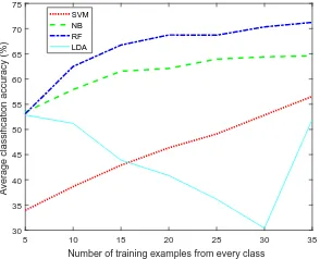
Fig.1 shows the average cross-validation classification ac-curacies of the for classifiers across different size of training set. As can be seen, the highest improvement for SVM, NB, and RF was obtained by increasing the number of training trials from 5 to 10 per class. Thereafter, for the SVM classifier the improvement is continued and the maximum accuracy is obtained by using all 35 trials per class in training. For NB and RF, the maximum accuracy is nearly achieved by using 30 trails per class for training. Interestingly, in NB and RF, the improvement in the average accuracy is less the 2% after using 20 trails per class for training. LDA behaved differently compared to the other classifiers where the maximum accuracy was achieved with less training data
and the accuracy degraded until having 30 trials in training. Thereafter, the average accuracy increased with 35 training trials from every class. Using few training data, we can not have optimal LDA classifier [24]. As a result, the well-know problem of LDA classifier: the singularity of the within-class scatter matrix appears and several studies in the literature emerges to solve this problem as in [23]. As a result, the reliable results of LDA starts with having 35 trials in training as the number of training trials (175) becomes more than the number of features (144).
For the TF data, the improvement in accuracy was evaluated from two perspectives: training size, and frame length. Similar to the MC data, the training size was varied, however, each analysis was repeated using different imagination time frames as the trial length (i.e. 0.5, 1, 1.5, 2, 2.5, 3, 3.5, and 4 seconds immediately started from the beginning of the imagination). In Fig.2, the behaviour of each classifier is presented. As expected, for SVM, NB and RF the average accuracy increases with the increase of training size regardless of the length of the time frame. Interestingly, increasing the length of the time frame also leads to an increase in the accuracy, although the results of the 3.5 and 4 sec time frames are very closed (0.3 % average difference). The relation between the increase in the time frame and the improvement in the classification accuracy can be justified as a longer time frame could improve the estimation of DWT. This might be similar to the concept of wavelet zero-padding [25] as we performed baseline correction and the participants were instructed to perform the imagination at the beginning of the time frame and have clear mind after that. As a result, the end part of the time frame is most-likely similar to adding zeros to the end of the time frame. Further investigation is needed to prove this hypothesis. Similar trend is observed for all the classifiers except LDA, perhaps because LDA is more affected by training size as previously explained for the MC data.
5 10 15 20 25 30 35
Number of training examples from every class 30
35 40 45 50 55 60 65 70 75
Average classification accuracy (%)
[image:5.612.363.510.485.604.2]SVM NB RF LDA
Fig. 1. Average 10-fold classification accuracy (%) using different training sizes for MC data using different classifiers.
C. The relation between repetitions order and classification accuracy
Number of training examples from every class
Average classification accuracy (%)
5 10 15 20 25 30 35
20 40 60 80
100 Support Vector Machine
5 10 15 20 25 30 35
20 40 60 80
100 Naiive Bayes
5 10 15 20 25 30 35
20 40 60 80
100 Random Forest
5 10 15 20 25 30 35
20 40 60 80
100 Linear Discriminant Analysis
[image:6.612.348.529.249.284.2]0.5 second 1 second 1.5 seconds 2 seconds 2.5 seconds 3 seconds 3.5 seconds 4 seconds
Fig. 2. Average classification accuracy (%) of the TF data in classifying 5 imagined words, using different classifiers, when different training sizes and different time frames are used
each block is proportional to the size of the block. From Table III we can observe that the maximum average accuracy achieved is 60.7% using RF and total number of training 270 trials. In comparison to Table I, if we use data from the same block and 175 trials we can obtain 69.3% average classification accuracy using RF. Moreover, in comparison to Fig 1 62.5% using RF is achieved using 50 total training trails. However, having each word recorded in one separate block leads to a high temporal correlation in EEG patterns across different words. Thus, recording using sub-blocks or random representation is more representative as the temporal correlation is reduced in EEG patterns of each class. This issue has been investigated in [3].
D. The effect of imagination time on classification accuracy
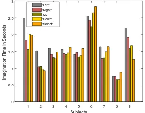
In the MC data, the participant determined the start and the end of the imagination trial using mouse clicks. Fig. 3 shows the average time needed for each participant to imagine every word. Across subjects, the average imagination length for the five words are: 1.8, 1.5, 1.3, 1.5, and 1.6 seconds for the words: “Left”, “Right”, “Up”, “Down”, and “Select” respectively. As shown in Table IV, adding the imagination length as an extra feature improves the average classification accuracy for all the classifiers by an average of (2% - 4%), which means that the imagination length is possibly an effective
TABLE III
10-FOLDS AVERAGE CLASSIFICATION ACCURACY TO CLASSIFY BETWEEN FIVE WORDS FORMCSEPARATED DATA;USING TRAINING AND TESTING
DATA MIXED FROM TWO DIFFERENT BLOCKS FOR EACH WORD.
Subject
Average classification accuracy [SVM] [NB] [RF] [LDA] S1 52.3 50.6 68 48 S2 51.6 41 53 50.6 S3 41.6 46.6 57.3 46.3 S4 53.6 57.3 72.6 50.6 S5 29.3 31.3 46.3 38.3 S6 58.3 44.3 73.6 56.6 S7 49.6 49 52.3 46.6 S8 41 49.3 59.3 38 S9 40.6 37.3 64.3 43 Average 46.4 45.1 60.7 46.4
TABLE IV
10-FOLD AVERAGE CLASSIFICATION ACCURACY(%)USING DIFFERENT FEATURES FORMCDATA BY USING35TRAINING TRIALS FOR EVERY
WORD.
Feature SVM NB RF LDA
DWT 52.7 61.7 69.3 49.6 Imagination length 35.4 34.8 28.5 34.8 DWT and Imagination length 56.6 64.3 71.4 47.9
feature for classifying the words. However, applying t-test shows that for none of the classifiers this improvement is statically significant. Importantly, the examination of how the imagination length for each word may vary across blocks recorded needs to be investigated because the learning curve might affect how the subjects perform the imagination task.
In Table V we examined the effect of having subject specific TF. This TF was adopted by reducing the fixed time frame to a length that is approximately equal to the maximum average length the participant needed in mouse click separated imagination for any of the imagined words (from figure 3). In Comparison to the classification accuracies in Table I, the results are statically significant only for RF classifier in comparison to MC word separation. This also approves what we explained in section IV-B that long fixed time frame provides low frequencies in the extracted time window to help in distinguishing EEG patterns related to speech.
1 2 3 4 5 6 7 8 9 Subjects
0 0.5 1 1.5 2 2.5 3
Imagination Time in Seconds
[image:6.612.359.509.526.643.2]"Left" "Right" "Up" "Down" "Select"
Fig. 3. Average imagination time in second using 40 trials from every word
V. CONCLUSION
TABLE V
10-FOLDS AVERAGE CLASSIFICATION ACCURACY TO CLASSIFY BETWEEN FIVE WORDS WHERE FOR EACH SUBJECT THE TIME FRAME IS ADOPTED TO THE AVERAGE TIME FRAME FOR THE WORD WITH THE MAXIMUM LENGTH
INMC
Subject
Average length of the word with maximum length
Fixed time frame [SVM] [NB] [RF] [LDA]
S1 2.5 54.8 67.9 86 45.3
S2 1.5 60.7 64.2 72.8 53.9 S3 1.5 54.8 66.8 69.7 56.8 S4 1.5 55.7 85.3 91.4 62.2 S5 1.5 43.3 64.3 68.3 46.2
S6 3 87.4 79.9 91.9 75.3
S7 1.5 59.8 63.3 79.9 54.3
S8 1 71.8 91.5 92.4 65.4
S9 2.5 38.2 55.2 65.3 32.6 Average 1.8 58.5 70.9 79.74 54.6
trials separated using mouse click and fixed time frame. First, we examined the relation between training size (5-35 trials) and the classifier performance using the dataset collected by imagining 5 different words and 4 classifiers. Due to the limitation in the collected number of trials for each word, we did not observe any saturation in the classification across different number of training trials. However, the results show that the rate of improvement in accuracy gets very small when we move from 25-35 training trials for each class. On contrast, this improvement is increasing sharply when we increase the training from 5-15 trials for every class. For all training sizes and both data separation methods, Random Forest classifier provides the highest average classification accuracy. Second, for fixed TF separation, we found that the longest time frame provides DWT features that lead to best results. In our results 3.5-4 seconds gives the maximum average accuracy. Third, the system was trained using data from two blocks recorded in the same session but more training trials needed to get equivalent performance to classification using one block. Finally, the use of MC to separate the words showed that the imagination speech rate was less than real spoken speech as the participants needed 1.8 seconds on average to imagine the longest word even after removing the time needed to do mouse click (on average 100 ms for male adults [26] ).
Future work will include the examination of random words presentation instead of blocks. In [3], it has been discussed that the recognition of random words is difficult. This examination will involve the classification accuracy as well as answering how the word randomization will affect the extracted features.
REFERENCES
[1] C. Brunner, R. Leeb, G. M¨uller-Putz, A. Schl¨ogl, and G. Pfurtscheller,
“Bci competition 2008–graz data set a,”Institute for Knowledge
Dis-covery (Laboratory of Brain-Computer Interfaces), Graz University of Technology, pp. 136–142, 2008.
[2] P. Suppes, Z.-L. Lu, and B. Han, “Brain wave recognition of words,”
Proceedings of the National Academy of Sciences, vol. 94, no. 26, pp. 14 965–14 969, 1997.
[3] A. Porbadnigk, M. Wester, and T. S. Jan-p Calliess, “Eeg-based speech recognition impact of temporal effects,” 2009.
[4] E. F. Gonz´alez-Casta˜neda, A. A. Torres-Garc´ıa, C. A. Reyes-Garc´ıa, and L. Villase˜nor-Pineda, “Sonification and textification: Proposing methods
for classifying unspoken words from eeg signals,” Biomedical Signal
Processing and Control, vol. 37, pp. 82–91, 2017.
[5] M. DZmura, S. Deng, T. Lappas, S. Thorpe, and R. Srinivasan, “Toward
eeg sensing of imagined speech,” inProceeding of International
Con-ference on Human-Computer Interaction. Springer, 2009, pp. 40–48. [6] N. Yoshimura, A. Satsuma, C. S. DaSalla, T. Hanakawa, M.-a. Sato, and
Y. Koike, “Usability of eeg cortical currents in classification of vowel
speech imagery,” inProceeding of International Conference on Virtual
Rehabilitation (ICVR). IEEE, 2011, pp. 1–2.
[7] N. Miller, G. Maruyama, R. J. Beaber, and K. Valone, “Speed of speech
and persuasion.”Journal of personality and social psychology, vol. 34,
no. 4, p. 615, 1976.
[8] M. Wester, “Unspoken speech-speech recognition based on
electroen-cephalography,”Master’s Thesis, Universitat Karlsruhe (TH), 2006.
[9] T.-G. A. Antonio, R.-G. C. Alberto, and V.-P. Luis, “Toward a silent
speech interface based on unspoken speech,” inProceeding of the 5th
International Joint Conference on Biomedical Engineering Systems and Technologies, 2012.
[10] S. Zhao and F. Rudzicz, “Classifying phonological categories in
imag-ined and articulated speech,” inProceeding of the Acoustics, Speech and
Signal Processing (ICASSP). IEEE, 2015, pp. 992–996.
[11] M. Matsumoto and J. Hori, “Classification of silent speech using support
vector machine and relevance vector machine,”Applied Soft Computing,
vol. 20, pp. 95–102, 2014.
[12] A. R. Sereshkeh, R. Trott, A. Bricout, and T. Chau, “Online eeg
classi-fication of covert speech for brain-computer interfacing,”International
Journal of Neural Systems, p. 1750033, 2017.
[13] H. H. Jasper, “The ten twenty electrode system of the international
fed-eration,”Electroencephalography and clinical neurophysiology, vol. 10,
pp. 371–375, 1958.
[14] G. F. Woodman, “A brief introduction to the use of event-related
potentials in studies of perception and attention,”Attention, Perception,
& Psychophysics, vol. 72, no. 8, pp. 2031–2046, 2010.
[15] A. Subasi, “Eeg signal classification using wavelet feature extraction and
a mixture of expert model,”Expert Systems with Applications, vol. 32,
no. 4, pp. 1084–1093, 2007.
[16] R. E. Yohanes, W. Ser, and G.-b. Huang, “Discrete wavelet transform
coefficients for emotion recognition from eeg signals,” inIn proceeding
of International Conference of the IEEE Engineering in Medicine and Biology Society (EMBC). IEEE, 2012, pp. 2251–2254.
[17] L. Angrisani, P. Daponte, M. D’apuzzo, and A. Testa, “A measurement
method based on the wavelet transform for power quality analysis,”IEEE
Transactions on Power Delivery, vol. 13, no. 4, pp. 990–998, 1998. [18] A. R. Sereshkeh, R. Trott, A. Bricout, and T. Chau, “Eeg classification
of covert speech using regularized neural networks,”IEEE/ACM
Trans-actions on Audio, Speech, and Language Processing, vol. 25, no. 12, pp. 2292–2300, 2017.
[19] L. Guo, D. Rivero, J. A. Seoane, and A. Pazos, “Classification of eeg signals using relative wavelet energy and artificial neural networks,” in Proceedings of the first ACM/SIGEVO Summit on Genetic and Evolutionary Computation. ACM, 2009, pp. 177–184.
[20] F. Lotte, M. Congedo, A. L´ecuyer, F. Lamarche, and B. Arnaldi, “A review of classification algorithms for eeg-based brain–computer
interfaces,”Journal of neural engineering, vol. 4, no. 2, p. R1, 2007.
[21] G. H. John and P. Langley, “Estimating continuous distributions in
bayesian classifiers,” inProceedings of the 11th conference on
Uncer-tainty in artificial intelligence. Morgan Kaufmann Publishers Inc., 1995, pp. 338–345.
[22] P. Kumar, R. Saini, P. P. Roy, P. K. Sahu, and D. P. Dogra,
“Envi-sioned speech recognition using eeg sensors,”Personal and Ubiquitous
Computing, vol. 22, no. 1, pp. 185–199, 2018.
[23] R. Huang, Q. Liu, H. Lu, and S. Ma, “Solving the small sample size
problem of lda,” inProceeding of the 16th International Conference on
Pattern Recognition., vol. 3. IEEE, 2002, pp. 29–32.
[24] P. P. Markopoulos, “Linear discriminant analysis with few training data,” inProceeding of the Acoustics, Speech and Signal Processing (ICASSP). IEEE, 2017, pp. 4626–4630.
[25] J. Pardey, S. Roberts, and L. Tarassenko, “A review of parametric
modelling techniques for eeg analysis,”Medical engineering & physics,
vol. 18, no. 1, pp. 2–11, 1996.
[26] S. Komandur, P. W. Johnson, and R. Storch, “Relation between mouse
button click duration and muscle contraction time,” inProceeding of 30th