Relations for Improved SAT Encodings of Pseudo-Boolean Constraints
.
White Rose Research Online URL for this paper:
http://eprints.whiterose.ac.uk/148518/
Version: Accepted Version
Proceedings Paper:
Ansótegui, Carlos, Bofill, Miquel, Coll, Jordi et al. (7 more authors) (Accepted: 2019)
Automatic Detection of At-Most-One and Exactly-One Relations for Improved SAT
Encodings of Pseudo-Boolean Constraints. In: Proceedings of the 25th International
Conference on Principles and Practice of Constraint Programming. Springer . (In Press)
[email protected] https://eprints.whiterose.ac.uk/ Reuse
Items deposited in White Rose Research Online are protected by copyright, with all rights reserved unless indicated otherwise. They may be downloaded and/or printed for private study, or other acts as permitted by national copyright laws. The publisher or other rights holders may allow further reproduction and re-use of the full text version. This is indicated by the licence information on the White Rose Research Online record for the item.
Takedown
If you consider content in White Rose Research Online to be in breach of UK law, please notify us by
Exactly-One Relations for Improved SAT
Encodings of Pseudo-Boolean Constraints
⋆Carlos Ans´otegui1
, Miquel Bofill2
, Jordi Coll2
, Nguyen Dang3
, Juan Luis Esteban4
, Ian Miguel3
, Peter Nightingale5
, Andr´as Z. Salamon3
, Josep Suy2
, and Mateu Villaret2
1
University of Lleida, Lleida, Spain
2
University of Girona, Girona, Spain
{miquel.bofill,jordi.coll,josep.suy,mateu.villaret}@imae.udg.edu
3
University of St Andrews, St Andrews, United Kingdom
{nttd,ijm,Andras.Salamon}@st-andrews.ac.uk
4
Technical University of Catalonia, Barcelona, Spain
5
University of York, York, United Kingdom
Abstract. Pseudo-Boolean (PB) constraints often have a critical role in constraint satisfaction and optimisation problems. Encoding PB con-straints to SAT has proven to be an efficient approach in many applica-tions, however care must be taken to encode them compactly and with good propagation properties. It has been shown that at-most-one (AMO) and exactly-one (EO) relations over subsets of the variables can be ex-ploited in various encodings of PB constraints, improving their compact-ness and solving performance. In this paper we detect AMO and EO relations completely automatically and exploit them to improve SAT encodings that are based on Multi-Valued Decision Diagrams (MDDs). Our experiments show substantial reductions in encoding size and dra-matic improvements in solving time thanks to autodra-matic AMO and EO detection.
Keywords: Automatic CSP reformulation·SAT·pseudo-Boolean· at-most-one constraint.
1
Introduction
Solving constraint satisfaction and optimisation problems often requires dealing with Pseudo-Boolean (PB) constraints, either explicitly stated in the original
⋆
model or as a product of some reformulation process. A successful approach to solving constraint problems is by translation to SAT and the use of SAT solvers. Example tools that support this method include MiniZinc [24, 18], Picat [28], and Savile Row [25]. Ideally, such encodings would be compact (in terms of the number of clauses and additional variables) and would have good propagation properties.
In this paper we focus on efficiently translating PB constraints to SAT within Savile Row, which produces a reformulated SAT model from an input constraint model in the Essence Prime language [26]. There exist several approaches for compactly encoding PB constraints to SAT based on different representations, such as Decision Diagrams [13, 2], Sequential Weight Counters [17], Generalised Totalisers [19], and Polynomial Watchdog schemes [5].
There are also attempts to exploit collateral constraints to shrink these en-codings further [1, 8]. In particular, in [8], it is shown how to use existing At-Most-One (AMO) and Exactly-One (EO) relations on subsets of the variables of a PB constraint to obtain very compact decision diagram-based representations. In that work, the authors provide empirical evidence of the utility of using this technique in several scheduling problems. Specifically, they provide specialised SAT Modulo Theories (SMT) encodings exploiting AMO and EO relations. How-ever, these relations are found by hand and are not always obvious.
In this work we propose a technique for exploiting such collateral constraints when encoding PB constraints to SAT in a fully automatic manner. By collat-eral constraints we mean constraints that are derived from the entire model in some way. They may appear directly in the model, or they may be implied by constraints in the model. One can then use a declarative constraint modelling language and forget about collateral constraints when posting PB constraints. The proposed system is able to automatically identify AMO and EO relations and to take them into account when encoding PB constraints. In particular, we use the approach described in [3] to detect sets of Boolean variables in a SAT formula that model finite-domain variables, which essentially corresponds to de-tecting the AMO (i.e., cardinality constraints with≤operator andk = 1) and At-Least-One (ALO) relations among a set of Boolean variables. Later, in [7], a method to detect arbitrary cardinality constraints (k≥ 1) was introduced. To the best of our knowledge, [7] is the first attempt to apply in practice reformula-tion techniques through the automatic detecreformula-tion of cardinality constraints. They reformulate the input SAT formula by erasing the clauses entailed by the cardi-nality constraints detected so far. In our work, we tackle a different goal since our aim is to use the automatically detected cardinality constraints to improve the encoding of more general constraints, specifically PB constraints.
used to deduce sub-clauses from implication graphs, and also unit propagation was used in [14] to detect redundant clauses in SAT formulas.
We apply the technique to several problem classes and highlight the charac-teristics of each regarding the automatically found AMO and EO relations. Our experiments show dramatic improvements of encoding size and solving time.
2
Preliminaries
Essence Prime is typical of solver-independent constraint modelling languages in providing integer and Boolean variable types, as well as multidimensional matrices of these types. It supports arbitrarily nested arithmetic and logical constraint expressions, as well as a suite of global constraints. Savile Row is able to translate any Essence Prime model into SAT, which we define here.
A Boolean variable is a variable than can take truth values 0 (false) and 1 (true). A literal is a Boolean variable x or its negation¬x. A clause is a dis-junction of literals. A propositional formula in conjunctive normal form (CNF) is a conjunction of clauses. Any propositional formula can be transformed into CNF.
A CNF formula represents a Boolean function, i.e. a function of the form
f :{0,1}n
→ {0,1}. Anassignment is a mapping of Boolean variables to truth values, which can also be seen as a set of literals (e.g., {x= 1, y = 0, z = 0} is usually denoted {x,¬y,¬z}). A satisfying assignment of a Boolean function
f is an assignment that makes the function evaluate to 1. In particular, an assignmentAsatisfies a CNF formulaF if at least one literall of each clause in
F belongs toA. Such an assignment is called amodel of the formula.
SAT is the problem of determining if there exists a satisfying assignment for a given propositional formula. Given two formulasF andG, we say that Gis a logical consequence ofF, writtenF |=G, iff every model ofF is also a model of
G. We say that two Boolean functionsF andGare logically equivalent, denoted
F ≡G, ifF |=GandG|=F.
Unit propagation (UP) is the core deduction mechanism in modern SAT solvers: whenever each literal of a clause but one is false, the remaining literal must be set to true in order to satisfy the clause. We say that G is a logical consequence of F by UP, writtenF |=UP G, iff F∧ ¬Gcan be determined to be unsatisfiable by UP.
Savile Row encodes integer variables to provide SAT literals for (x=a) and (x ≤ a) for each integer variable xand value a. Each constraint type is then encoded using these SAT literals, as described in [25]. For this work we have added the MDD encoding of PB constraints as defined below.
Definition 1. A pseudo-Boolean (PB) constraint is a Boolean function of the formPni=1qili⋄K whereK and theqi are integer constants, li are literals, and ⋄ ∈ {<,≤,=,≥, >}.
x1
x2 x2
x3 x3
x4
T F
1 0
1
0
0
1
1 0
0 1
0 1
x1, x2
x3, x4
F T
x2
x1, else
[image:5.612.135.418.83.275.2]x4 x3, else
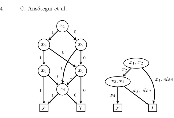
Fig. 1.Left: BDD forP = 2x1+ 3x2+ 4x3+ 5x4 ≤7; Right: MDD forP, assuming
AM O(x1, x2) andAM O(x3, x4), where eachxibranch means choosingxi= 1, and the
else branches mean choosingxi= 0 for allxiin the corresponding source node.
Definition 3. An at-least-one (ALO) constraint is a Boolean function of the formPni=1li≥1, where all li are literals.
Definition 4. An exactly-one(EO) constraint is a Boolean function of the form
Pn
i=1li= 1, where all li are literals.
One of the best methods to encode PB constraints to SAT is to use Binary Decision Diagrams (BDDs) [13]. In [2] an even more efficient encoding is given for PB constraints where all coefficients, literals and K are positive and the relational operator is≤. Such a constraint has the important property of being
monotonic decreasing, i.e. any model remains a model after flipping inputs from 1 to 0. In [8] it is shown how the encoding can be dramatically reduced in size in the presence of AMO constraints over subsets of the variables. The improved encoding is based on Multi-Valued Decision Diagrams (MDDs) and is intended also for monotonic decreasing PB constraints. Figure 1 shows an example of this situation. The number of nodes and edges in the second diagram is substantially reduced, and the number of clauses and variables needed to encode the diagram is reduced accordingly. The input of this encoding is a PB constraint, and a partition of its literals, where each part must satisfy an AMO constraint. We will refer to each of the parts as an AMO group.
3
Background: AMO and ALO Detection
In this section we present the approach described in [3] to semantically detect AMO and ALO constraints in a SAT formulaF. The idea is to compute for each literal inF which other literals are entailed by unit propagation (UP). Then an undirected graphG= (V, E) is constructed, where all verticesu∈V are literals ofF and an edge (u, v)∈E iffF∧u|=UP¬v, i.e.F∧u∧ ¬vcan be determined to be unsatisfiable by UP. In other words, if (u, v) ∈ E then F |= (¬u∨ ¬v), therefore there is an AMO constraint between literalsuandv. We refer to these AMO constraints between two literals as mutexes. Accordingly, we refer to the graph Gas theUP-mutex graph ofF.
Recall that a clique of a graphG= (V, E) is a subset of vertices of Gsuch that every pair of vertices u, v are adjacent, i.e. (u, v) ∈ E. Therefore, every cliqueC= (V′, E′) in the UP-mutex graph of a SAT formulaF corresponds to an AMO A =Pv∈V′v ≤ 1 such that F |=A. By construction, we know that
there is a mutex between all pairs of literalsu, v∈V′, henceF|=u+v≤1 and so F |=Pv∈V′v ≤1. Thus we can identify all the AMO constraints in a SAT
formulaF that can be detected by UP by finding the cliques in the UP-mutex graph of F.
In [7] the authors propose an approach to detect cardinality constraints (Boolean functions of the formPni=1li≤kwhere allli are literals andk≥1 is
an integer) which generalize AMO constraints. As pointed out by the authors, this methodology is particularly useful fork >2, compared to other approaches for detecting cardinality constraints.
Given a set of literals L of a formula F we can also automatically detect whetherF |=UP∨l∈Ll, i.e.F entails by UP an ALO constraint onL, by testing whetherF∧Vl∈L¬lis unsatisfiable by UP.
There are two key details in the procedure we have described to semantically detect the AMO constraints in a SAT formula F. First of all, how do we detect the mutexes, i.e. the level of local consistency (power of propagation) we use to find them. Notice that by enforcing stronger consistency than UP we may identify more mutexes and consequently more AMO constraints. Second, how do we detect the cliques in the UP-mutex graph. Depending on the goal of the particular application, the challenge is to properly address these two key details. In the following section, we adapt this procedure to our context by replacing the SAT formula F with a CSP instance, replacing unit propagation with the propagation of the constraint solver Minion [15].
4
AMO and EO Relations in Savile Row
groups will arise either from the decomposition of an integer variable, or from the detection of a clique of mutexes in the mutex graph. As described in [25] Savile Row performs two tailoring processes, the first of which uses the constraint solver Minion [15] to filter variable domains, and the second produces output for the desired solver (SAT in this case). Our approach adds mutex detection to Minion, and finds AMO and EO groups during the second tailoring process.
4.1 Mutex Inference
The mutex inference step is performed on Minion’s CSP representation of the problem at hand. This representation contains integer constraints that will be transformed into PB constraints later. These integer constraints are of this form Pn
i=1qiei⋄K. An expressionei may be an integer variable, a Boolean literal, or
(xi⋄ki) wherexi is an integer variable or a Boolean literal. Next, any Boolean expressions of the form (xi⋄ki) are replaced with a new Boolean variablebi and the constraint bi ↔(xi⋄ki) is added to the model. By adding thebi variables, the mutex detection algorithm is able to see the mutex betweenx <5 andx≥5 for example.
Minion is called to perform domain filtering [25] and to find mutexes between literals of Boolean variables. For each Boolean variablebin the CSP, each value of
bis assigned in turn and the propagation loop of Minion is called. Consequences of the assignment are propagated through the entire constraint model, includ-ing integer variables and global constraints. All assignments of other Boolean variables (to either 0 or 1) by propagation are recorded in the mutex graphG.
Mutex inference is very similar to [3] (described in Section 3) with the SAT formula replaced by the CSP, and unit propagation replaced by Minion’s propa-gation algorithms. Comparing propapropa-gation power is not straightforward because it depends on the SAT encoding on the one hand, and fine details of propagators on the other. However, there is one key advantage to using the CSP representa-tion: we avoid generating the (potentially very large) encoding of the problem instance without considering AMO and EO relations. See, for example, the Nurse Scheduling Problem (Section 5.3) where the encoding that uses AMO and EO relations is ten times smaller than the one without.
4.2 Normalisation
To use the MDD encoding referred to in Section 2 we must have monotonic decreasing PB constraints in ≤form. Reformulations are required both before and after the AMO and EO groups are constructed. In the first step, all PB and sum constraints are rearranged into the form Pni=1qiei ≤ K with arithmetic
transformations [13].
Termsqieiwhereeiis integer are dealt with as follows. Letq=qiande=ei. First, if q <0, thenq← −q ande← −e. Second, if the smallest possible value
e=kiby enumerating all valueskiexcept the smallest value, andKis adjusted accordingly.
At this point, all expressionsei in the constraint are Boolean. All termsqiei where qi <0 are made positive by replacing withqi(1− ¬ei), then multiplying out and subtracting the constant from both sides. The constraint is now a mono-tonic decreasing≤PB constraint, suitable for encoding to SAT via an MDD as described in Section 2. However, the next steps may require inverting the polar-ity of some Boolean expressionsei in order to match the detected AMOs, losing the normal form. In this case, the normal form will be restored after making the polarities match.
4.3 AMO and EO Detection
For each PB constraint, we take the subgraphG′= (V′, E′) of the mutex graph G where V′ is a set containing both literals of all Boolean variables in the constraint. The algorithm has a list of verticesL, initially containing all vertices in V′. Lis sorted by descending degree in G′. A clique cover is constructed by iterating a greedy clique finding algorithm. To construct one clique, the algorithm takes the first vertex fromLthen adds as many as possible other vertices in the order of L, breaking ties (where the degree is equal) by choosing the vertex whose coefficient is most common within the clique (as a heuristic to reduce the number of outgoing edges of the corresponding nodes in the MDD). Whenever a vertexvis added to a clique, bothvand¬vare removed fromL. The end result is a clique cover containing one literal of each Boolean variable in the constraint. For each clique in the cover, a new AMO or EO group is built as follows. If the negations of literals in the clique correspond with negations in the PB constraint (or the clique has one literal) then we do (1), otherwise (2).
1. The AMO group is constructed directly from the clique. If all literals in the group form an EO corresponding to an integer variable (i.e. literals corre-spond to (x= a) or ¬(x6= a) for all valuesa of some integer variablex), then we can exploit the EO relation to reduce the size of the group. We delete the term(s) with the smallest coefficientc, and subtractcfromKand from the other coefficients within the AMO group.
2. If the negation of the termqiei does not match the literal in the clique, the term is rewritten asqi(1− ¬ei) (and rearranged as above), creating a term with a negative coefficient. Once all terms of the group have the appropriate sign, an EO is created by making a new Boolean variableb(constrained to be true iff all expressionsei in the group are false) and adding a term 0bto the group. All coefficients within the group andK are adjusted by subtracting the smallest coefficient. Terms with coefficient zero are removed to create an AMO group.
then the AMO group is smaller than the clique. Each AMO group detected in this way will be added to the model as an AMO constraint.
We find EO groups by a syntactic check in case (1) above. EO groups can also be detected semantically using propagation (Section 3), and the semantic approach may find more EO groups. In our case this would involve calling Minion a second time, with more overhead than the syntactic check.
4.4 Reformulation Example
In this section we give an example of the normalisation and reformulation process that illustrates the described steps and cases. Suppose we have a CSP instance C with the following variables:
– xwhich is an integer variable with domain{1,2,3};
– ywhich is an integer variable with domain {−2,−1,0,1}; and
– zandt that are Boolean variables.
SupposeChas the following two constraints to be translated to SAT:
C1: 2(x= 1) + 4(x= 2) + 3(x= 3)−3y+ 4z+ 5t≤13
C2:¬z∨ ¬t
Before performing the mutex inference, we replace each of the expressions of the form (x⋄k) with a Boolean auxiliary variable b, and add the constraint
b↔(x⋄k).C1 is replaced with the following four constraints:
b1↔(x= 1)
b2↔(x= 2)
b3↔(x= 3)
C3: 2b1+ 4b2+ 3b3−3y+ 4z+ 5t≤13
The inference mechanism described in Section 4.1 detects the following mutexes, where the first three come from the decomposition of integer variablex, and the last one is due to constraintC2:
¬b1∨ ¬b2 ¬b1∨ ¬b3 ¬b2∨ ¬b3 ¬z∨ ¬t
The following two AMO relations are inferred from the above mutexes:
b1+b2+b3≤1
z+t≤1
These two AMO relations are added to the model as AMO constraints.
An EO relation is detected amongb1,b2, andb3, as described in Section 4.3.
smallest coefficient inC3 (b1 in this case), and adjusting the coefficients of the
other terms (as described in Section 4.3). The two Boolean variables z and t
form an AMO group. Finally, the integer variabley with four values will form an AMO group of three terms, as described in Section 4.2.
C3 is reformulated intoC4 as follows:
C4: 2b2+ 1b3+ 9[y=−2] + 6[y=−1] + 3[y= 0] + 4z+ 5t≤14
Note that the right hand side constant has been adjusted to 14, and the coef-ficients of the terms corresponding to xandy have been adjusted as well. The variables ofC4 are partitioned into the following three AMO groups:
{b2, b3}
{[y=−2],[y=−1],[y= 0]} {z, t}
If the AMO and EO detection process is enabled, the SAT encoding has 18 variables and 33 clauses. Without the detection, it has 33 variables and 53 clauses. The SAT encoding of the MDD derived from C4 has only 7 clauses,
whereas the MDD derived from the constraint without AMO and EO detection (which has only one non-singleton AMO group derived fromy) is encoded with 37 clauses.
5
Experimental Evaluation
In this section we evaluate our approach on four diverse case studies: Combina-torial Auctions (CA), the Multi-Mode Resource-Constrained Project Scheduling Problem (MRCPSP), the Nurse Scheduling Problem (NSP), and the Multiple-Choice Multidimensional Knapsack Problem (MMKP). Each of these problem classes have AMO and EO relations that could be identified by expert modellers, and we show that our system is able to identify them without any human ef-fort. The effects on the size and solving time of the resulting SAT formula are dramatic.
All problems except MRCPSP use a PB objective function. To abstract solv-ing performance from any particular optimisation process of the PB objective function, we converted CA, NSP and MMKP problem classes into decision prob-lems. Specifically, we bound the objective function with the best known value of the objective function, so we are searching for a solution that is as good as the best known solution.
For the decision problems CA, NSP, and MMKP, we use the Glucose 4.1 SAT solver [4]. For MRCPSP, where we minimise an integer variable, we use the MaxSAT solver Open-WBO version 2.0 [23], which uses Glucose 4.1 as its core SAT solver. All the experiments were run on an 8GB IntelR
XeonR
In our experiments we use three configurations. The first (PB) has no AMO or EO detection, however normalisation is always applied when encoding a con-straint via an MDD (Section 4.2). The second configuration (PB(AMO)) per-forms AMO detection but not EO detection (i.e. the EO check in step (1) of Section 4.3 is switched off). The third configuration (PB(EO)) has both AMO and EO detection.
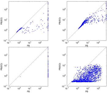
[image:11.612.133.482.231.536.2]Reported solving times include both reformulation preprocessing and time spent by the SAT solver.
Fig. 2.Scatter plots comparing the median of the solving time among all 10 executions for each instance in the dataset. From left to right and top to bottom: CA, MRCPSP, NSP, MMKP.
5.1 Combinatorial Auctions
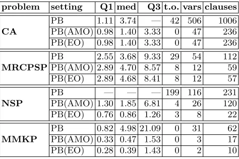
Table 1. Summary statistics of configurations PB, PB(AMO) and PB(EO) for the four case studies. — indicates time out.
problem setting Q1 med Q3 t.o. vars clauses
CA
PB 1.11 3.74 — 42 506 1006 PB(AMO) 0.98 1.40 3.33 0 47 236 PB(EO) 0.98 1.40 3.33 0 47 236
MRCPSP
PB 2.55 3.68 9.33 29 54 112 PB(AMO) 2.89 4.70 8.57 8 12 59 PB(EO) 2.89 4.68 8.41 8 12 57
NSP
PB — — — 199 116 231
PB(AMO) 1.30 1.85 6.81 4 26 120 PB(EO) 0.76 0.86 1.26 3 8 22
MMKP
PB 0.82 4.98 21.09 0 31 62 PB(AMO) 0.33 0.47 1.53 0 3 17 PB(EO) 0.28 0.39 1.43 0 2 10
Every bidder makes an offer for a set of items (a package), and it has to be decided whether to sell the whole package to the bidder. It is not allowed to sell only a proper subset of the demanded items. A natural viewpoint to model the problem is to introduce a Boolean variablesold[b]for each packageb, that states whether it is sold or not. Then, the decision version of the problem can be stated as:
forAll b1: int(1..nBids-1) . forAll b2: int(b1+1..nBids) .
incompBids[b1,b2] -> (!sold[b1] \/ !sold[b2]),
(sum b : int(1..nBids) .
sold[b] * profit[b] ) >= lb
wherenBidsis the number of bids,profit[b]is the bid value for packageb, incompBids[b1,b2] is true when two bids have a non-empty intersection, and lbis the minimum total profit that is required.
The first constraint ensures that no item is sold in two different packages, or equivalently that every item is sold in at most one package. This will allow Savile Row to detect mutexes between variables sold[b]where packages share some item. Typically the sets of packages that contain each particular item will not be disjoint, so the clique cover finding algorithm plays an especially important role when reformulating this problem.
5.2 MRCPSP
The Multi-mode Resource-Constrained Project Scheduling Problem (MRCPSP) is an iconic problem in the scheduling field [10]. The problem requires deciding a start time (schedule) and an execution mode (schedule of modes) for each job of a project. The jobs are non-preemptive, i.e. they cannot be paused once they have started. Also, the jobs have demands over a set of resources, that can be either renewable, i.e. the amount of resource assigned to a job is recovered once the job finishes, or non-renewable, i.e. availability is not restored when jobs finish. For each job, its duration and its demands depend on the chosen execution mode. The schedule must ensure that a given set of precedence relations between jobs are all satisfied, that the given availability of renewable resources is never surpassed during the execution of the project, and that the given availability of non-renewable resources is enough to supply the demands. Moreover, the project completion time (makespan) must be minimised.
We model the resource constraints as follows. We introduce an auxiliary integer variablemode[j]for each jobj, which represents the selected execution mode for jobj. To deal with renewable resources constraints we also introduce a Boolean variablejobActive[j,m,t]for each jobj, execution modemand time instant twithin a scheduling horizon, which is constrained to be true iff job i is running in mode mat time t. The renewable resource constraints are:
forAll t: int(0..horizon) . forAll res: int(1..resRenew) . (
sum j: int(1..jobs) .
sum m: int(1..nModes[j]) .
jobActive[j,m,t]*resUsage[j,m,res] ) <= resLimits[res]
We model non-renewable resource constraints as:
forAll res : int(resRenew+1..nRes) . ( sum j: int(1..jobs) .
sum m: int(1..nModes[j]) .
(mode[j]=m) * resUsage[j,m,res] ) <= resLimits[res]
wherehorizonis a scheduling horizon which accepts a valid schedule (if the instance is satisfiable),1..resRenewandresRenew+1..nResare the sets of re-newable and non-rere-newable resources respectively,1..jobsis the set of all jobs, 1..nModes[j]is the set of available execution modes for jobj,resUsage[j,m,res] is the consumption of job j on resource res when it runs in mode m, and resLimits[res]is the availability of resourceres.
execution mode, and if an activity precedes another they will never run in par-allel. Further, two modes of a pair of activities are incompatible if the combined demands for the two modes surpass the availability of some resource.
For this problem we have used the 552 satisfiable instances of the j30 dataset, which is the hardest from PSPLib [21]. These instances contain projects of 30 activities, 3 possible execution modes for each activity, 2 renewable resources and 2 non-renewable resources.
5.3 NSP
The Nurse Scheduling Problem (NSP) is the problem of finding an optimal as-signment of nurses to shifts per day considering some coverage and shift prefer-ence constraints. There are plenty of variants of this problem depending on the constraints considered [12, 27]. In this work we consider the basic version of the problem where solutions must satisfy all shift coverage constraints, i.e. each shift and day must have a certain number of nurses assigned, and must satisfy the constraint that each nurse only works a certain number of days per week, and must minimise the total penalisation according to the preferences of the nurses. PB constraints appear in the Essence Prime model when bounding the total amount of penalisation allowed. We use integer variable nS[n,d] to state the shift assignment of each nursenand dayd, and the penalisation constraint is as follows:
(sum n: int(1..nNurses) . sum d: int(1..nDays) .
sum st: int(1..nShiftTypes) . (nS[n,d]=s) * p[n,d,st] ) <= ub
wherenNursesis the number of nurses,nDaysthe number of days,nShiftTypes the number of shift types andp[n,d,st]is the penalty of assigning shift stto nursenon day d. Finally, since we are computing the decision version of NSP, ub is the maximum cost allowed. Notice that EO relations occur among the penalties for each nurse and day, since nSranges over integer values from 1 to nShiftTypes.
In this work we consider a set of instances from NSPLib, a repository of thousands of NSP instances grouped into classes by several complexity indica-tors. Details can be found in [27]. We focus on a sample of 200 instances taken uniformly and independently at random from the N25 Set: 25 nurses, 7 days and 4 shift types (including the free shift). Each instance has a minimum number of nurses required per shift and day, and includes the nurses preferences to work on each shift and day (a penalty is between 1 and 4, where 1 is the rank of the most preferred shift).
5.4 MMKP
capacity-bounded dimensions, it is required to pack exactly one item of each class without surpassing the knapsack capacities. Each item of each class has a given profit, and a weight in each dimension. It is also required to maximise the profit of the chosen items [20]. The decision version of the problem requires that the profit is greater than or equal to a lower boundlb.
The PB constraints appear in our Essence Prime model when bounding ca-pacities and profit. We use integer variablesitem[c]to state which item of class chas been chosen. The constraints are as follows:
forAll d: int(1..nDimensions) . ( sum c: int(1..nClasses) .
sum i: int(1..classSize) . (item[c]=i) * weight[c,i,d] ) <= cap[d],
(sum c: int(1..nClasses) . sum i: int(1..classSize) .
(item[c]=i) * profit[c,i] ) >= lb
wherenDimension is the number of dimensions,nClassesis the number of classes,classSizeis the number of items in each class (n.b. in this dataset all classes have the same number of items),weight[c,i,d]is the weight of itemi of classcfor dimensiond,cap[d]is the capacity of dimensiond, profit[c,i] is the profit of itemiof classcandlbis the minimum profit to be achieved.
Notice that EO relations occur becauseitemranges over integer values from 1 toclassSize.
For conducting the experimental evaluation we have chosen the 1983 satis-fiable instances from the 2000 instances of dataset (10-5-5-G-R-W) from [16], that contain 10 classes of 5 items each, and the knapsack has 5 dimensions. This dataset turns out to be reasonably hard in comparison to others from the same work that appear to be easy for SAT solvers.
5.5 Experimental Results
Figure 2 compares total time (including reformulation and solving) of PB and PB(EO) for every instance of each problem class. The solving time improvements are remarkable for all four problem classes. There are improvements between one and two orders of magnitude in many cases between PB and PB(EO), although there is a small overhead on some of the easiest instances.
6
Conclusion and Future Work
We have presented a fully automatic approach to find and exploit at-most-one (AMO) and exactly-one (EO) relations in SAT encodings of PB constraints. The approach is integrated into Savile Row, a constraint modelling tool that can automatically produce a SAT encoding of any constraint model written in the language Essence Prime. Until now, AMO and EO relations have been exploited for this purpose only in problem-specific encodings constructed by experts. Results show dramatic improvements in SAT formula size and solving time on four problem classes.
In future work we will explore stronger inference mechanisms for the detection of mutexes, which could lead to larger and more effective AMO relations. We also plan to study whether we can reformulate PB constraints more efficiently through detection of cardinality constraints with k≥2 applying the approach in [7].
References
1. Ab´ıo, I., Mayer-Eichberger, V., Stuckey, P.J.: Encoding linear constraints with implication chains to CNF. In: CP: Principles and Practice of Constraint Pro-gramming. pp. 3–11. LNCS 9255, Springer (2015). https://doi.org/10.1007/978-3-319-23219-5 1
2. Ab´ıo, I., Nieuwenhuis, R., Oliveras, A., Rodr´ıguez-Carbonell, E., Mayer-Eichberger, V.: A new look at BDDs for pseudo-Boolean constraints. Journal of Ar-tificial Intelligence Research pp. 443–480 (2012). https://doi.org/10.1613/jair.3653 3. Ans´otegui, C.: Complete SAT solvers for Many-Valued CNF Formulas. Ph.D.
the-sis, University of Lleida (2004)
4. Audemard, G., Simon, L.: On the Glucose SAT solver. Interna-tional Journal on Artificial Intelligence Tools 27(1), 1–25 (2018). https://doi.org/10.1142/S0218213018400018
5. Bailleux, O., Boufkhad, Y., Roussel, O.: New encodings of pseudo-Boolean con-straints into CNF. In: SAT: Theory and Applications of Satisfiability Testing. pp. 181–194. LNCS 5584 (2009). https://doi.org/10.1007/978-3-642-02777-2 19 6. Biere, A.: Lingeling. SAT Race (2010)
7. Biere, A., Le Berre, D., Lonca, E., Manthey, N.: Detecting cardinality constraints in CNF. In: SAT: Theory and Applications of Satisfiability Testing. pp. 285–301. LNCS 8561, Springer (2014). https://doi.org/10.1007/978-3-319-09284-3 22 8. Bofill, M., Coll, J., Suy, J., Villaret, M.: Compact MDDs for Pseudo-Boolean
9. Bofill, M., Palah´ı, M., Suy, J., Villaret, M.: Solving Intensional Weighted CSPs by Incremental Optimization with BDDs. In: CP: Principles and Prac-tice of Constraint Programming. pp. 207–223. LNCS 8656, Springer (2014). https://doi.org/10.1007/978-3-319-10428-7 17
10. Brucker, P., Drexl, A., M¨ohring, R., Neumann, K., Pesch, E.: Resource-constrained project scheduling: Notation, classification, models, and methods. European Jour-nal of OperatioJour-nal Research112(1), 3–41 (1999). https://doi.org/10.1016/S0377-2217(98)00204-5
11. Darras, S., Dequen, G., Devendeville, L., Mazure, B., Ostrowski, R., Sa¨ıs, L.: Using Boolean constraint propagation for sub-clauses deduction. In: CP: Principles and Practice of Constraint Programming. pp. 757–761. LNCS 3709, Springer (2005). https://doi.org/10.1007/11564751 59
12. De Causmaecker, P., Vanden Berghe, G.: A categorisation of nurse rostering prob-lems. Journal of Scheduling 14(1), 3–16 (2011). https://doi.org/10.1007/s10951-010-0211-z
13. E´en, N., Sorensson, N.: Translating pseudo-boolean constraints into SAT. Jour-nal on Satisfiability, Boolean Modeling and Computation 2, 1–26 (2006), http://satassociation.org/jsat/index.php/jsat/article/view/18
14. Fourdrinoy, O., Gr´egoire, ´E., Mazure, B., Sa¨ıs, L.: Eliminating redundant clauses in sat instances. In: CPAIOR: Integration of AI and OR Techniques in Constraint Programming for Combinatorial Optimization Problems. pp. 71–83. LNCS 4510, Springer (2007). https://doi.org/10.1007/978-3-540-72397-4 6
15. Gent, I.P., Jefferson, C., Miguel, I.: Minion: A fast scalable constraint solver. In: ECAI: European Conference on Artificial Intelligence. Frontiers in Arti-ficial Intelligence and Applications, vol. 141, pp. 98–102. IOS Press (2006), http://www.booksonline.iospress.nl/Content/View.aspx?piid=1654
16. Han, B., Leblet, J., Simon, G.: Hard multidimensional multiple choice knapsack problems, an empirical study. Computers & Operations Research37(1), 172–181 (2010). https://doi.org/10.1016/j.cor.2009.04.006
17. H¨olldobler, S., Manthey, N., Steinke, P.: A compact encoding of pseudo-Boolean constraints into SAT. In: KI 2012: 35th Annual German Conference on Artificial In-telligence. pp. 107–118. LNCS 7526, Springer (2012). https://doi.org/10.1007/978-3-642-33347-7 10
18. Huang, J.: Universal Booleanization of constraint models. In: CP: Principles and Practice of Constraint Programming. pp. 144–158. LNCS 5202, Springer (2008). https://doi.org/10.1007/978-3-540-85958-1 10
19. Joshi, S., Martins, R., Manquinho, V.: Generalized totalizer encoding for pseudo-Boolean constraints. In: CP: Principles and Practice of Constraint Program-ming. pp. 200–209. LNCS 9255, Springer (2015). https://doi.org/10.1007/978-3-319-23219-5 15
20. Kellerer, H., Pferschy, U., Pisinger, D.: Multidimensional knapsack problems. In: Knapsack Problems, pp. 235–283. Springer (2004). https://doi.org/10.1007/978-3-540-24777-7 9
21. Kolisch, R., Sprecher, A.: PSPLIB - A Project Scheduling Problem Li-brary. European Journal of Operational Research 96(1), 205–216 (1997). https://doi.org/10.1016/S0377-2217(96)00170-1
22. Leyton-Brown, K., Shoham, Y.: A test suite for combinatorial auctions. In: Com-binatorial auctions, chap. 18, pp. 451–478. The MIT Press (2006)
24. Nethercote, N., Stuckey, P.J., Becket, R., Brand, S., Duck, G.J., Tack, G.: Miniz-inc: Towards a standard CP modelling language. In: CP: Principles and Prac-tice of Constraint Programming. pp. 529–543. LNCS 4741, Springer (2007). https://doi.org/10.1007/978-3-540-74970-7 38
25. Nightingale, P., Akg¨un, ¨O., Gent, I.P., Jefferson, C., Miguel, I., Spracklen, P.: Automatically improving constraint models in Savile Row. Artificial Intelligence
251, 35–61 (2017). https://doi.org/10.1016/j.artint.2017.07.001
26. Nightingale, P., Rendl, A.: Essence’ description. arXiv:1601.02865 (2016), https://arxiv.org/abs/1601.02865
27. Vanhoucke, M., Maenhout, B.: NSPLib: a nurse scheduling problem library: a tool to evaluate (meta-)heuristic procedures. In: Brailsford, S., Harper, P. (eds.) Operational research for health policy: making better decisions. pp. 151–165. Peter Lang (2007)