Design of generalized minimum variance controllers for nonlinear multivariable systems

Design of Generalized Minimum Variance Controllers

for Nonlinear Systems

Michael J. Grimble

Abstract: The design and implementation of Generalized Minimum Variance control laws for nonlinear multivariable systems that can include severe nonlinearities is considered. The quadratic cost index minimised involves dynamically weighted error and nonlinear control signal costing terms. The aim here is to show the controller obtained is simple to design and implement. The features of the control law are explored. The controller obtained includes an internal model of the process and in one form is a nonlinear version of the Smith Predictor.

Keywords: Cost-function, delays, minimum variance, nonlinear, optimal control.

1. INTRODUCTION

The proposed control law is for nonlinear multivariable systems is based on a rich heritage. Åström introduced the Minimum Variance (MV) controller assuming the linear plant was minimum phase and later derived the MV controller for processes that could be non-minimum phase (Åström 1979 [1]). The latter was guaranteed to be stable on non-minimum phase processes, whereas the former was unstable. Hastings-James and later Clarke and Hastings-James (1971, [2]), modified the first of these control laws by adding a control costing term. This was termed a Generalized Minimum Variance (GMV) control law and enabled non-minimum phase processes to be stabilized, although when the control weighting tended to zero the control law reverted to the initial algorithm of Åström, which was unstable (Grimble 1981 [3], 1988 [4]). However, the control law had similar characteristics to Linear Quadratic Gaussian (LQG) design and in some cases and was much simpler to implement. This simplicity was exploited in the GMV self-tuner (1975, [5]). All of these results were applicable to linear discrete-time processes.

The aim in the following is to first introduce the

GMV controller for Nonlinear (NL) multivariable processes using dynamic cost-function weightings in the same spirit as the above results. The structure of the system is defined so that a simple controller and solution are obtained. When the system is linear the results then revert to those for the GMV controller (Grimble 2001 [8]).

There is some loss of generality in assuming the reference and disturbance models are represented by linear subsystems. However, the plant model can be in a very general nonlinear operator form, which might involve state-space, transfer operators or even nonlinear function look up tables. That is, the input sub-system to the plant might include valves or a servo-system that has no traditional equation based model. The input nonlinear subsystem can be a black box. No state-space or model based operator structure is needed. The optimal solution reveals all that is needed is a method of computing the output from such subsystem, given a control input. If on the an equation based model is available it may be used directly. For this reason the nonlinear part of the plant is represented in operator (unstructured form) for most of the analysis.

The nonlinear (NL) dynamic terms, in the plant, only need to be open loop stable and can include hard static nonlinearities or complex dynamic equations. The ability to introduce very general plant structures, without formal models, is an advantage of the method. This feature is similar to the properties of some controllers generated by feedback linearization methods (Goodwin, Rojas and Takata, 2001 [6]). However the plant model does not need to be affine in the control and feedback linearization methods do not of course provide a general solution that gives optimal disturbance rejection and tracking.

For linear systems stability is ensured when the combination of a control weighting function and an

__________

Manuscript received October 29, 2005; accepted February 20, 2006. Recommended by Editorial Board member Jae Weon Choi under the direction of past Eitor-in-Chief Myung Jin Chung. This work was supported by the Engineering and Physical Science Research Council (EPSRC), grant No: EP/C526422/1. We would like to acknowledge the discussions and work by Pawel Majecki on the development of a comprehensive toolbox for implementing the algorithms and the example.

error weighted plant model is strictly minimum phase. For nonlinear systems a related operator equation must have a stable inverse. It is shown that if there exists say a PID controller that will stabilize the nonlinear system, without transport delay elements, then a set of cost weightings can be defined to guarantee the existence of this inverse and thereby ensure the stability of the closed loop.

The results presented here concentrate on the feedback control problem and design/implementation issues. It only includes an abbreviated solution since the full solution of the Feedforward and Tracking Nonlinear Generalized Minimum Variance (NGMV) control problem was given in Grimble (2005 [11]). This required the solution of three bilateral Diophantine equations in [11]. The structure of the polynomial equations derived below, is rather different to those in [11] and for the feedback control here only one unilateral Diophantine equation is involved. The result is a truly nonlinear controller that is sufficiently straightforward to be used on real applications. In the following the properties of the control law are explored and the focus is on implementation and design issues.

2. SYSTEM DESCRIPTION

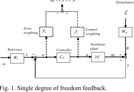
The system description is of restricted generality and is carefully chosen so that simple results are obtained. The plant itself is nonlinear and may have quite a general form. However, the reference and disturbance signals are assumed to have linear time-invariant model representations. This is often valid, since in many applications the only models available for the disturbance and reference signals are LTI approximations. The system is shown in Fig. 1 and includes the nonlinear plant model and the linear reference/disturbance models. There is no loss of generality in assuming that the zero mean white noise sources { ( )}ω t and { ( )}ξ t have identity covariance matrices. There is no requirement to specify the distribution of the noise sources, since the special structure of the system leads to a prediction equation, which is dependent upon the linear disturbance and reference models.

The polynomial matrix system models, for the multivariable system, shown in Fig. 1, may now be introduced. Part of the system is represented by linear models. The linear disturbance, reference and plant output subsystem models have the left-coprime polynomial matrix representation:

1 1 1 1 1 1 1 1

0 0

[ (W z_d −),W z_r( −),W z_k(−)]=A z−(−)[ (C z_d −),E z_r( −),B z_k(−)]. (1) The polynomial matrix system models follow:

Disturbance model: W_d(z−1)= A−1(z−1)C_d(z−1)

Reference model: W z_r( −1) = A−1(z−1)E z_r( −1).(2)

The subsystem associated with the plant inputs is assumed to be unstructured and of the form:

Nonlinear plant model:

(

Wu t

)( )

=D_k

(

W_ku t

)( )

,(3)

where _diag

{

-k1_, -k2_,..., -kr

}

k

D = z z z denotes the common

delay elements in the respective output signal paths. One of the main strengths of the method is that no model is required for the nonlinear subsystem:

(

W_ku t

)( )

. It is necessary to have some means of computing the output from this block but a traditional equation based model is not essential. That is, look-up tables may be employed, old Fortran code may be available that enables the output to be computed for a given input, or as in current research, a fuzzy-neural model, may be fitted to plant data. These methods do not involve a conventional model.

Most of the results do not need a more detailed breakdown of the plant model structure. However, if the plant model is separated into an input subsystem W1k and a linear subsystem W0k then only the input nonlinear subsystem needs to be assumed stable (finite gain stable for example). In the later sections, to show the system can be stabilised, it will be assumed that any unstable modes of the linear plant subsystem are included in a stable/unstable linear time-invariant block of polynomial matrix form:

-1 0k 0k.

W =A B The delay free plant model:

(

W_ku_฀

)( )

t

(

)( )

0k 1k

W u t

= W -1

(

)( )

0k 1k

A B u t

= W _฀ and the total

plant model:

(

Wu t

)( )

=D Wk 0k

(

W1ku

)

( )t , (4)

where it is assumed that this nonlinear model W_1k is finite gain stable. Note the solution does not require the plant model be affine in the control. The signals shown in the system model of Fig. 1 may be listed:

Error signal: e t

( ) ( )

=r t −y t

( )

, (5)

Plant output:

y t

( )

=d t

( ) (

+ Wu t

)( )

, (6)

Reference: r t

( )

=W_rω

( )

t ,

(7)

Disturbance signal: d t

( )

=W_dξ

( )

t ,

(8)

Combined signal: f t

( ) ( )

=r t −d t

( )

.

(9)

The power spectrum for the combined reference – disturbance:

* *

ff = rr+ dd=W Wr r +W Wd d

(10)

and the spectral-factor Y_f satisfies:

*

f f ff

where the system models ensure Yf is strictly minimum phase. A measurement noise model has not been included to simplify the equations. This is appropriate so long as the control cost-function weighting, ensures controller roll-off at HF.

3. NONLINEAR GMV CONTROL PROBLEM

[image:3.595.308.543.65.497.2]

The optimal NGMV control problem involves the minimisation of the variance of the signal

{

φ₀

( )

t

}

in

Fig. 1. This has a (r m× ) dynamic cost-function weighting matrix: Pc(z-1) on the error signal, represented by linear polynomial matrices as:

1

c cd cn

P =P P− . The signal also includes an m-square, nonlinear dynamic control signal costing operator term:

(

F_cu t

)( )

. Typically Pc is low-pass and Fc is

a high-pass transfer. The signal:

( )

(

)( )

0( )t P e tc cu t

φ = + F (12)

is to be minimized in a variance sense, so the cost:

( ) ( )

{

0T 0

}

{

{

0

( ) ( )

0T

}

}

J =E φ t φ t =E trace φ t φ t , (13)

where E

{}

⋅ denotes the unconditional expectation

operator. If the smallest of the delays in each output channel of the plant are of magnitudes:

{

k k₁, ₂,...,k_r

}

, respectively, this implies the control signal at time t affects the jthoutput at least k_j steps later. For this

reason the control signal costing can be defined as:

(

Fcu

)( )

t =Dk

(

Fcku

)( )

t . (14)

Typically this will be a linear operator but it may be nonlinear to cancel the plant input nonlinearities in appropriate cases. The control weighting operator

ck

F is assumed full rank and invertible.

Theorem 3.1: NGMV Optimal Controller

The NGMV optimal controller to minimize the variance of the weighted error and control signals may be computed from the following equations. The assumptions are made that the input subsystem W_1k is finite gain stable and the nonlinear operator

(

PcWk−F฀ck

)

has a finite gain stable causal inverse,

due to the choice of weighting operators P_c and F_c. The smallest degree solution:(G F₀, ₀), with respect to F₀, must be computed from the polynomial matrix unilateral Diophantine equation:

0 0

p cd k cf f

A P F +D G =P D , (15)

where the left coprime polynomial matrices satisfy:

1 1

p cf cn

A P− =P A− (16)

and the spectral factor: Y_f =A D−1 _f.

Optimal control signal: The optimal NGMV

control action can be computed as:

( )

(

₁

)

1

(

)

1 ₁

( )

0 f k ck pf cd 0 f .

u t = F Y− − − ⎛_⎜ A P − G Y −e t⎞_⎟

⎝ ⎠

฀

฀

W F (17)

฀ Proof: Involves collecting results in next section.

฀

The solution is simplified if Dk and weighting Pc and Yf commute. This assumption is valid if the delay elements are the same in each channel D_k =z−kI or if Pc, Yf are diagonal. The class of problems considered are those for which a solution to the Diophantine equation can be found where the row degrees of F (₀ z−1) are less than the delay path magnitudes

{

k k₁, ₂,...,k_r

}

and this is ensured under

the conditions listed in the previous remark.

4. NGMV NONLINEAR OPTIMAL CONTROL

A simple optimisation argument is used in the following. The signal to be minimised is shown to consist of both linear and nonlinear terms. However, the stochastic part of the problem involves linear models so that a prediction equation may easily be derived. This enables the signal to be written in terms of future and past white noise related terms. The optimal causal solution is therefore that which sets the past terms to zero. This will include some of the nonlinear terms and the optimal control follows.

Consider the minimisation of φ₀

( )

t that represents

the weighted sum of error and control signals and is the same dimension as the input signal. This fictitious or inferred output is defined as: φ₀

( )

t =P e t_c

( )

+

(

Fcu t

)( )

, where Pc is assumed to be a linear and Fc

can be a linear or nonlinear operator. Now from the equations in §2: = − = − −e r y r d Wu and hence,

Pc

Wr

Wd

r + e u

-

y d

W +

+ m Fc

Disturbance

Control weighting

Reference Error weighting

+ + ξ

C0

Nonlinear plant Controller

0 P ec cu

φ = +F

ω

[image:3.595.311.535.73.227.2]

( )

(

)

0 t P rc( d) Pc c u

φ = − − _{W F}− _฀ . (18)

Assumption: An important assumption will now be

recalled that does not affect stability properties. That is, the model for signal f = −r d is assumed linear.

Spectral factor: Recall the innovations model for the signal: f =Y_f , where Yf is a linear transfer and

( )

t denotes a zero mean white noise signal of identity covariance matrix. This follows from a spectral-factor computation, given the disturbance Wd and the reference Wr signal models. The Yf=A-1Df where from the system description Df is strictly Schur. Thence, from the first term in (18): P r_c

(

−d

)

=P f_c

-1 1

cd cn f

P P A D−

= . Introduce the left coprime matrices

Ap and Pcf whereP Acn 1 A Pp1 cf

− ₌ −

then Pcf =

(

)

1

p cd

A P −

cf f

P D and from (15) the weighted error and control

signals:

(

)

-1

(

)

0 A Pp cd P Dcf f Pc c u

φ = − _{W F}− . (19)

Introduce the Diophantine equation, to expand the combined disturbance and reference model into two groups of terms:

0 0

p cd k cf f

A P F +D G =P D , (20)

where the solution for

(

F G₀, ₀

)

satisfies the row j

degree of F₀<k_j. Hence,

(

)

-1

(

)

1

0 0

c f p cd cf f p cd k

P Y = A P P D =F + A P − D G .(21)

The first polynomial matrix includes delay elements

in the jth channel, up to and including z− +kj 1 and the last term involves delay elements greater than or equal to k_j in each channel. Substituting into (19):

(

)

-1

(

)

0 F0 A Pp cd D Gk 0 Pc c u

φ = + − W F− (22)

but =Y_f−1f =Y_f−1(r−d)and substituting in (22):

(

)

-1 ₁

0

F

0

A P

p cd

D G Y

k 0 f

e

φ

=

+

−

(23)

(

) (

-1

)

₁

0

p cd k p cd c f f c

A P D G A P P Y Y− u

⎛ ⎞

+_⎜ − + _⎟

⎝ W F ⎠

but A P P Y_{p cd c f} =A P A D_{p cn} −1 _f =P D_{cf f} and hence

(20) gives: D G_{k 0}−P D_{cf f} = −A P F_{p cd 0}.

These last two equations then give the desired weighted error and control signal as:

(

)

-1 ₁

(

₁

)

0 F0 A Pp cd D G Yk 0 f e c F Y0 f u

φ = + − + F − −W_฀ .(24)

The control signal at time t affects the jth system output at time t+kj and hence the control signal costing term F_c should include a delay of kj steps, so that F_c=D_kF_ck. Moreover, since in general the control signal costing is required on each signal channel, the F_ck weighting may be defined to be of full rank and invertible. (24) may be simplified further if A P_{p cd} and Dk and F Y0 f−1 and Dk commute,

which is certainly the case under the assumptions on Pc and Yf discussed after the Theorem at the end of the last section. From (24) the inferred or fictitious output may be written as:

( )

( )

( )

1

(

)( )

0 t F0 t Dk[( cku t) F Y0 f ku t

φ = + F − − W

1 1

0

(A P_{p cd})− G Y_f− e t( )]

+ _฀ . (25)

To compute the optimal control signal inspect the form of the weighted error and control signals in equation (25). Since the row degrees of F₀ are required to be less than kj (the magnitude of the delay in the jth channel) the jth row of the first term is dependent upon the values of the white noise signal components:

( )

t ,…,

(

t−k_j +1 .

)

The remaining terms in the expression for the jth row are all delayed by at least kj steps and therefore depend upon the earlier values:

(

t−k_j

)

,

(

t−k_j −1 ,

)

and it follows the first and remaining terms are statistically independent. The first term on the right of (25) is independent of the control action and the smallest variance is achieved when the remaining terms are zero. The optimal control signal must satisfy:

(

)( )

(

)

1

( )

1 1 1

0 0

( ) _{ck f k p cd f}

u t = − _⎝⎛⎜F Y− u t − A P − G Y− ฀e t ⎞⎟_⎠

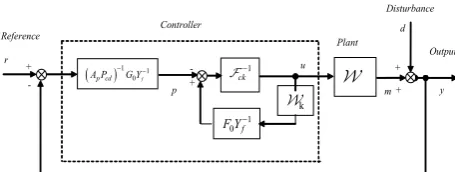
฀ F W (26)

and this may be represented by the Fig. 2. Note the signal φ₀ =P e_c +F_cu =P r_c

(

−y

)

+F_cu involves a weighting F_c that normally has a negative zero frequency gain. The forward path gain of the controller block is therefore usually positive.

Reference

Output

( )1 1

0f

p cd

A P −G Y−

1 0 f

F Y−

1

ck− F

y

+

-

r

Disturbance d

+

u

- +

Controller

W

k W

Plant

+

[image:4.595.311.539.646.732.2]

m p

An alternative expression for the control signal, in terms of the exogenous signals may be found that is useful for stability analysis. From (26), recalling

1 0 f

F Y− and D_k, commute, the optimal control:

( )

1 1

(

)

( )

0

[

ck f k

u t =F− F Y− W u t

(

)

1 ₁

(

( )

( ) (

)( )

)

0 ]

p cd f

A P − G Y− r t d t u t

− _฀ − − W

but 1

(

)

1 1 1

0 f p cd k 0 f cd cn.

F Y− + A P − D G Y− =P P− Thence,u t

( )

=F_ck−1

(

)

( )

(

)

1 ₁

(

)( )

0

c k p cd f

P u t A P − G Y − r d t

⎛ _{− −} ⎞

⎜ ⎟

⎝ W ⎠.

Alternatively, rewriting:

( )

(

)

1

(

)

1 ₁

(

( )

( )

)

0

c k ck p cd f

u t = PW −F _฀฀− A P − G Y − r t −d t ,(27)

where the existence of a finite gain stable causal inverse of the nonlinear operator

(

P_cW_k −F_ck

)

ensures the control action represents a stable system.

The system output follows as: m t( )=

(

Wu t

)( )

and since the cascade controller sub-system

(

A P_{p cd}

)

−1

1 0 f

G Y − must be implemented in its minimal form, it

follows the output does not involve cancellation of any unstable modes present in W_0k(z−1) and internal stability is preserved.

5. IMPLEMENTATION OF CONTROLLER

Theimplementationof the controllershown in Fig. 2 reveals that the computational complexity increases with the model order and number of inputs and outputs since the plant model is included. A way to reduce part of this burden is described later (the RS version).

To consider the implementation of the control law recall from (17) that the optimal control signal is

given as:u t

( )

=

(

F Y_{0 f}−1W F_k− _ck฀฀

)

−1p t( ) where p t( )=

(

)

1 ₁

0 ( )

p cd f

A P − G Y − e t as shown in Fig. 2. Introducing

non-singular constant scaling matrix: Y0 the control signal may be written, using (4) as:

( )

_{1 1 1 1 1}

(

)

1 ₁

( )

0 0 0 1k 0 0 0

( f k ck) ( p cd f )

u t = Y−F D B− W −Y−F − Y− A P − G Y −e t and

(

)

1

1 1 1

0 0 0 1k 0 0

(Y−F D B−_{f k}W _฀−F_฀cy) ( )u t = A P Y_{p cd} − G Y_f−e t( ),(28)

where F ฀ F_ck=Y_{0 cy} and 1 1 1

0 0 0 1k

(Y− F D B−_{f k}W _฀−F_฀cy)− may then be computed, assuming the existence of the inverse F_cy-1 Redefine the scaled signal p(t) as:

( )

(

)

1 ₁

0 0 ( )

p cd f

p t = A P Y − G Y −e t

(

)( )

(

)

( )

1 1

0 0 f 0k 1k c y

Y− F D B− u t u t

= W − F . (29)

Then the control signal:

( )

1

(

1 1

(

)( )

( )

)

0 0 0k 1k .

cy f

u t =F − Y− F D B− W u t −p t

Unfortunately this solution requires iteration, since the right-hand side includes: ( ).u t This represents an algebraic loop and to avoid this problem the operator

1 1

0 0 0k 1k

(Y−F D B−_f W −F_฀฀cy) may be split into two parts involving a through term, without a delay N₀ and a term that depends upon past values of the control action, denotedz−1N₁. That is, p t

( )

=(Y₀−1F D₀ −_f1

1

0k 1k cy) ( 0 )( ) ( 1 )( )

B W −F_฀ u= N u t + z− N u t so that the

control:

( )

1

(

( )

1

)

0 ( 1 )( )

u t =N − p t − z− N u t . (30)

These results suggest the method of implementing the inverse operator in Fig. 3. To obtain a more explicit description of N₀ and N₁ let the nonlinear

plant model subsystem: W_1k =G₀+z−1G₁ and let the linear terms: Y₀−1F D B₀ −_f1 _0k =L₀+z L−1 ₁ where these nonlinear and linear terms G₀ and L₀ include no delay terms. Also let F_cy be split into a non-dynamic

through term: F_c0 and a term: z−1F_c1.That is, F_cy =

1

0 1

c +z− c

F F and

1 1

0 0 0k 1

( _{f k cy})

u = Y− F D B− − u

N฀ W F

(

1

)

0 0 cy ( 1 1 1k)

L z− L u

= G −F + G + W (31)

1

0 1

( u t)( ) (z− u t)( )

= N + N .

Hence identify: (N₀u t)( )=

(

L_{0 0}G −F_c0

)

u t( )

and (N₁u t)( )=(G₁+L₁W_1k −F_c1) ( )u t .

(32)

It is clear the algebraic loop is removed in the implementation of the inverse operator in Fig. 3. Note

1k

W

cy

F

1 0

−

N

1 1

0 0 f 0k

Y F D B− −

Plant and weighting operators _{Inverse operator}

+ _ _

u u

+

p

1 1

[image:5.595.313.537.652.737.2]

z−N

that this term L0 is not diagonal naturally and complicates the computation of N₀-1 which involves the inverse of the operator:

(

L_{0 0}G −F_c0

)

.

This can be simplified if an appropriate scaling is used as described below. Let Y0 denote the constant full rank matrix: Y0 = F0(0)Df(0)−1B0k(0),then this

may be used to normalise and diagonalise the fist z0 term in the denominator of the expression for the optimal control in (28). It is interesting that the scaling matrix Y0 may be related to the weighted plant model, by noting from (15) and (16):

1 1 1 1 1

0 f cd p k 0 f c

F D− +P− A D G D− − =P A−

and this gives:

1

0 0(0) f(0) 0k(0) c(0) 0k(0)

Y =F D − B =P W . (33)

Recall that in the previous section the term Y₀−1

1 0 f 0k

F D B− was expanded into a constant matrix and

terms that are delayed by at least one step:

1 1 1

0 0 f 0k 0 1

Y− F D B− =L +z L− (34)

but when the scaling (33) is applied the constant matrix: L₀=I. Clearly F_c0 can also be taken as a diagonal matrix function so that in the majority of problems the operator term:

(

)

0 0 0 0

(N u t)( )= LG −F_c u t( )=

(

G₀−F_c0

)

u t( )

in (32) is easy to invert, even noting that both of these terms may involve a nonlinear and multivariable process. The scaling suggested above ensures the direct control related terms have corresponding diagonal structures for most problems.

If it is complicated to compute the inverse of the non-dynamic function: N₀ a modified strategy can be applied. Assuming the existence of the inverse of

0

G and L0 (30) can be written, noting (31) as:

( )

1

(

( )

1

)

0 ( 1 )( )

u t =

N

− p t − z−

N

u t (35)

( )

(

)

1 1 1

0 0 1 0

( )− L− p t (z− u t)( ) _c u t( )

= G − N +F .(36)

The term F_c0 is often small so that although this expression involves an algebraic loop the result can considerably reduce the computation time. If the nonlinearity is represented by a black box the above method of avoiding the algebraic loop does not hold. In this case the function N₀ can be found by experiment, inputting a unit pulse at different operating points and fitting a smooth function. The operator N₁ can again be defined as: z−1N₁

0

=N −N but since errors are inevitable there remains the possibility of a small through term that will prolong an iterative solution of the inverse operator equations. To avoid this component a possible strategy, is to define the model with zeroed initial states/conditions as: F₀=N −N₀ and

compute the signal:

(

F₀u t

)( )

just for u at time t.

This can then be subtracted from the output of the block:

(

(N฀u t)( )−(N₀u t)( )

)

to ensure the error at the operating point is zero. Note that this complication is only introduced when black box models are used for the nonlinear subsystem and it may not be necessary.

The result (27) indicates a necessary condition for optimality is that the operator

(

P_cW_k −F_ck

)

must have a stable inverse. This reveals that one of the restrictions on the choice of cost weightings is that this stability condition be fulfilled. An important question is whether sensible choices of the weightings will lead to this condition. Consider the case where

ck

F is linear and F_ck = −F_k.Then,

(

)

(

1

)

c k k k k c k

PW +F u=F F− PW +I u (37)

and note that the term

(

I+F_k−1P_cW_k

)

represents the

return-difference for a system with controller:

1

c k c

K =F−P . (38)

This is important since it provides a starting point for cost weighting selection. That is, consider the delay free plant W_k and assume a PID controller exists Kc to stabilize the closed loop system. Then a weighting choice, that will ensure

(

P_cW_k +F_k

)

is stably

invertible, is F_k−1P_c =K_c. The controller expression may also be expressed in a slightly different form, using the inverse of the NL operator (from (26)) as:

( )

1 1

(

1 1

)

( )

0 0 1k 0

( _{f k ck}) ( _{p cd}) _f .

u t = F D B− W _฀−F − A P − G Y −e t

(39) The controller then has the structure shown in Fig. 4, showing the nonlinear compensator block.

Minimum Cost: This may be found from (25):

( )

( )

{

(

1

)

( )

0 t F0 t Dk ( ck F Y0 f k)u t

φ _{= + F −} −_W

(

)

1 ₁

( )

}

0

p cd f

A P − G Y− e t

+ _฀ (40)

and if at the optimum the term within the braces is null then φ_{0 min}

( )

t =F₀

( )

t and the minimum cost:

( )

(

)

(

( )

)

{

}

min 0 0

T

( ) ( )

_{1 1} *

0 0

| | 1

1 2

z

dz

trace F z F z

j z

π ₌ − −

⎧ ⎫

= _{⎨ ⎬}

⎩ ⎭

∫

. (41)

This expression for the minimum cost can provide a benchmark cost for nonlinear controller design and depends only on the reference and disturbance signal models that are linear, time invariant (LTI). This arises because the control action effectively removes the nonlinear plant model from the prediction of

{ }

φ( ) ,t whose variance is being minimised.

6. NONLINEAR SMITH PREDICTOR AND RESTRICTED STRUCTURE CONTROLLER

The optimal controller can be expressed in a similar form to that of a Smith Predictor. This provides a new nonlinear version of the Smith Predictor. Moreover, it provides an optimal method of tuning and provides optimal stochastic disturbance rejection and tracking properties. However, the introduction of this structure also limits the application of the solution on open-loop unstable systems. Although the structure illustrates a useful link between the new solution and the Smith time delay compensator, it also has the same disadvantage, that it may only be used on open-loop stable systems. The Nonlinear Smith Predictor will now be derived. Observe that the system in Fig. 2 may be redrawn as in Fig. 5. The changes are made to the linear subsystems by adding and subtracting equivalent terms. Now combine the two linear inner loop blocks, by first defining the signal:

( )

(

)( )

k k

m t = Wu t (42)

as follows:

(

)

1

1 1

0 f p cd 0 f k k

F Y − A P − G Y − D m

⎛ ₊ ⎞

⎜ ⎟

⎝ ⎠

(

) (

1

)

₁

0 0

p cd p cd k f k

A P − A P F D G Y −m

= + (43)

but from (20), assuming Dk and G0 commute:

1 1 1

0 0

(F Y_f− +(A P_{p cd})− G Y_f− D m_k) _k =P m_{c k}. (44)

[image:7.595.314.530.66.187.2]

The system may therefore be redrawn as shown in Fig. 6 where the control action clearly satisfies equation: (27). Now observe that the compensator may be rearranged, as shown in Fig. 7. This latter

structure is essential if Pc includes an integrator, which introduces integral action. That is, P_cd−1 must be placed in the inner error channel, rather than in individual blocks as in Fig. 6.

6.1. Restricted structure low order implementation The NGMV controller structure is already simple to understand and implement but in some industries the experience gained at using a PID parameterisation of a controller is so important it suggests replacing the cascade linear block by a low order parameterised model. This involves a parallel of the so-called Restrictive Structure (RS) control design method for linear systems introduced by Grimble (2000 [7]). The cascade linear subsystem in Fig. 1 can then be simplified to a given lower order controller structure where the cascade block is parameterised and the unknown coefficients optimised directly. This is Reference

( ₁ )1 0 f 0k 1k ck

F D B− W ฀−F −

Plant

- + e

r

+ +

u

W

( )1 ₁ 0f p cd

A P −G Y−

p

d

[image:7.595.58.293.66.136.2]

y

Fig. 4. Equivalent single DOF NL system.

1 ck − F 1 0f

F Y−

1 1

0

( ) f

p cd k

A P −G Y D−

Plant Compensator - _ 1 1 0

(A Pp cd)G Yf

− − ₊ y

+ +

+ _ +

r u

k D k m W _ k ฀ W y + + d

Fig. 5. Modification to the controller structure.

- + Plant - + k D

( )1 ₁ 0

p c d f

A P −G Y−

d + + W k W ψ + p c P 1 ck − F Compensator k m Output

r

-Disturbance

y

[image:7.595.311.536.220.334.2]

Reference

Fig. 6. Nonlinear smith predictor compensator.

_ + u Plant - + k D e - + + + p k W Compensator W 1 1 0 p f A G Y− −

Disturbance 0 ψ k m 1 1

ckPcd

− − F cn P Output Reference y r

Fig. 7. NL Smith predictor compensator and internal model (

0 Pcd

[image:7.595.315.536.371.482.2]

possible since the minimum cost expression, when the inner nonlinear block is unchanged, only depends upon the cascade term in the above figure. This may be shown since, from (27), the optimal control:

( )

(

)

1

(

)

1 ₁

(

( )

( )

)

0 .

c k ck p cd f

u t = P − − A P − G Y − r t −d t

฀

฀

W F

Denote the linear cascade block in Fig. 2 or Fig. 6 as:

1 1

0

(

)

c p cd _f

G

=

A P

−

G Y

− . If this block is to be simplified

by using a restricted structure then the parameterised cascade transfer (say a PID block) might be denoted as: G#_c and the sub-optimal control:

( )

_{( )} 1

(

( )

( )

)

c k ck c

u t# = PW −F − G# r t −d t . (45)

Substituting into (19), recalling P A_cn −1=A P_p−1 _cf,

(

)

-1

(

)

0 A Pp cd P Dcf f Pc c u

φ# = − W F− #

(

)

-1

(

( )

( )

)

(t)

p cd cf f k c

A P P D D G r t d t

= − # − (46)

(

)

= P_c−D G Y_k #_{c f} . (47)

The cascade block G#_c is linear and the output when this block is used is given by the linear system in equation: (47). It follows that the very same algorithms that has been used by Grimble (2002 [9]) for linear systems which directly optimises the cost index may be applied. Note that assuming that Dk commutes (44) reveals that as expected (47) simplifies to F₀ε( )t in the optimal (G_c =G#_c) case.

If greater simplification is demanded the inner nonlinear loop in Fig. 1 has to be simplified but in this case the nonlinear operator does not cancel when forming: (46). The problem is then no longer linear and the simple RS method does not apply. However, a so-called multiple model RS approach (Grimble 2002 [9]) has also been suggested for nonlinear systems. This technique may be applied to simplify the inner loop where the first step is to linearize the delay free plant model at a number of operating points. The single linear inner feedback loop block can then be calculated that minimises the cost function that is averaged over the different models. Note that the NL model for the plant is still included in the inner loop. Thus the controller remains nonlinear but with a simpler inner-loop linear sub-system. The resulting RS strategy should simplify the controller sub-systems simplify implementation.

7. NONLINEAR GMV CONTROL PROBLEM

The computation of a NGMV controller is illustrated below in the design of a scalar nonlinear discrete-time dynamic system, given in the following

very nonlinear state-space form:

1 2

1 ₂

1

2 2

1 2

2

( ) ( )

( )

( )

(

1)

( ),

1

( )

(

1)

x t x t

( ),

x t

x t

x t

u t

x t

x t

e

−

u t

⋅

+ =

+

+

+ =

+

(48)

1

( ) ( 4)

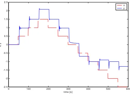
y t =x t− .

Let the initial state x(0) = 0. Observe that the output y(t) includes an explicit transport delay of k=5 samples. The open-loop system response to a series of steps is shown in Fig. 8, and the nonlinearity present in the system is clearly evident from the range of responses. The polynomial system models for the disturbance and reference models have the form: A = 1-1.79z-1 + 0.792z-2, Cd = 0.05-0.0495z-1, Er= 0.05 – 0.04z-1and Ap = A.

For the nonlinear GMV controller design, the linear reference model has been defined as: Wr = 0.05

(

1

)

1 0.99z− − , and is the stochastic analogue of a near

step reference changes. The model of the additive linear disturbance acting on the system output was

chosen as: W_d =0.05 1 0.8

(

− z−1

)

.

Assume the plant is controlled by the nominal stabilizing PID controller, denoted: C z₁( −1) , with filtered derivative term:

1 1

1 _{1 1}

(1 )

1

( ) 1

(1 ) (1 )

d

i d

T z

C z K

T z τ z

− −

− −

⎛ ₋ ⎞

= ⎜_⎜ + + ⎟_⎟

− −

⎝ ⎠and with the

tuning parameters: K=0.1, Ti=4s, Td=1s and

τ

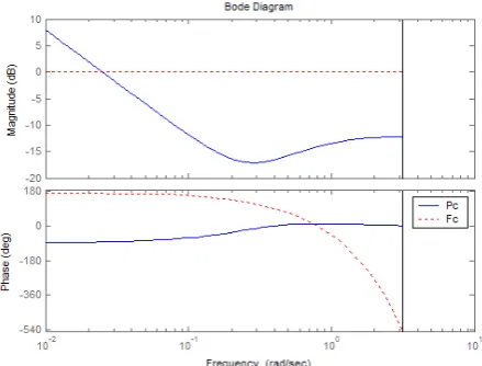
d=0.5.

As explained in Section 5.2, the initial choice of dynamic weightings for the NGMV design may be defined in terms of this controller as: P z_c( −1)=

1 1 4

1( ), c( ) .

C z− F z− = −z− The Bode plots of these weightings are shown in Fig. 9. The reference tracking of a sequence of steps for the two nominal controllers is shown in Fig. 10, and the corresponding output and control signal variances are collected in Table 1.

0 100 200 300 400 500 600

-2.5 -2 -1.5 -1 -0.5 0 0.5 1 1.5 2 2.5

tim e [s ]

u,

y

[image:8.595.320.533.586.739.2]

u y

Note that the nominal PID tuning parameters have only been found to stabilize the delay-free plant and are not optimized in any sense. However, this controller is useful in that it can provide initial design parameters for the NGMV controller that will stabilize the plant, ie. make the nonlinear operator stable and invertible.

Computation of NGMV control law: The cost

weightings implied by the PID controller become:

-1 -2

= 0.2250 - 0.3625 z + 0.15 z ,

cn

P

-1 -2

= 1.0000 - 1.5 z + 0.5 z ,

cd

P F_ck=1

and the polynomials in Fig. 2 have the solutions:

-1 -2 -3

0 = 0.0162 + 0.0133 z + 0.0125 z + 0.0127 z ,

F

-1 -2 -3

0 = 0.0134 - 0.0298 z + 0.0215 z - 0.0050 z ,

G

and Df = 0.0721-0.0621z-1. The optimal control may then be calculated from (26) or as in Fig. 2:

(

)( )

(

)

1

( )

1 1 1

0 0

( ) _{ck f k p cd f} .

u t = − ⎛_⎜F Y− u t − A P − G Y− e t ⎞_⎟

⎝ ฀ ⎠

฀ F W

(49) As can be seen from Fig. 10 and Table 1, the performance of the initial nonlinear controller design is close to that of the original PID, although it is normally more robust to the changes of the operating point (this can be seen for the set-point equal to zero). The stochastic performance of the nonlinear controller is also slightly better. The importance of this result is not the controller produced but that it provides a painless way to obtain an initial choice of cost weightings.

The nominal design may be modified by changing the control weighting. Parameterize the weighting as:

1

(1 )

ck

F = −ρ −γz− , where ρ is a positive scalar

and γ is a value from 0 to 1, to introduce a lead term. This is useful to reduce the high frequency gain of the controller. For the nominal design: ρ=1 and

0.

[image:9.595.319.529.67.233.2]

γ = The Bode plots are shown in Fig. 11. The parameterization of the weightings involves two tuning parameters and is meant to simplify the design. Decreasing the value of ρ (reducing the control Fig. 9. Frequency responses of the dynamic

[image:9.595.59.279.71.238.2]

weight-ings (nominal design).

[image:9.595.310.541.295.609.2]

Fig. 10. Time responses nominal PID and NGMV controllers.

Table 1. Stochastic performance: Nominal PID and NGMV controllers.

Op.

point Controller Var[e] Var[u] Var[phi] PID 0.01662 0.00117 0.00082 3

NGMV 0.01672 0.00104 0.00082

PID 0.01568 0.00046 0.00054 0

NGMV 0.01180 0.00025 0.00038

PID 0.01122 0.00168 0.00051 -1

NGMV 0.01117 0.00166 0.00052

PID 0.00729 0.00115 0.00035 -3

NGMV 0.00726 0.00115 0.00033

-20 -10 0 10 20 30

Ma

gni

tu

de

(

d

B

)

10-2 10-1 100 101

-540 -360 -180 0 180 360

P

h

as

e (

de

g)

Bode Diagram

Frequency (rad/sec)

γ ρ

weighting) leads to a faster response and a more violent control action. This can be seen from the stochastic performance results (with added disturbance noise). Interestingly, there is little change in the error variance. Decreasing ρ to a value of 0.35 leads to some undesirable oscillations. Adding a lead term resolves this problem. Fig. 12 and Table 2 present the simulation results for different values of ρ ( =0). Increasing ρ results in a slower response providing a simple tuning mechanism.

For comparison, the nominal PID controller has been retuned and compared with that of the NGMV controller with ρ= 0.5 and = 0.3.The results are presented in Fig. 13 and Table 3. After many attempts, a set of PID parameters were obtained close to the NGMV design in terms of speed of response, but the

NL plant still caused some oscillatory behaviour in the PID control design responses.

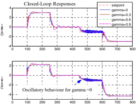
Fig. 14 and Table 4 present the simulation step response results for different values of (ρ=0.35, rescaled for constant DC gain).

In the last experiment, the plant time delay was increased from 4 to 10 samples. For the controller design, the same weightings were used as before but the NGMV controller obtained was of course different, reflecting the change in the time-delay. Then the Nonlinear Control Design Blockset of Matlab was used to find the optimal PID parameters, given the desired response. The boundary constraints were relaxed until a feasible set of parameters was found. However, it was not possible to tune the PID controller for satisfactory responses, across the whole operating range.

Fig. 15 shows the response of the NGMV design and 2 of the PID controllers obtained. The dynamic response of the NGMV controller is very close to that in Fig. 14, despite the significant increase in the time delay. It was not possible to obtain, for the PID controllers, both fast transient responses at the operating point = 3 and no oscillatory behaviour at the operating point = 0.

The PID controller did not have time delay compensation, so it might be argued that it is not a fair

0 100 200 300 400 500 600 700 800

-4 -2 0 2 4

Ou t p ut

Closed-Loop Responses

0 100 200 300 400 500 600 700 800

-4 -2 0 2

Co ntr ol

[image:10.595.314.536.67.238.2]

setpoint rho=0.5 rho=0.7 rho=1 rho=2

Fig. 12. Time responses for weighting parameters:

[image:10.595.56.286.68.234.2]

ρ= 0.5, 0.7, 1, 2; ( =0).

Table 2. Stochastic performance for weighting para-meters: ρ= 0.5, 0.7, 1, 2; = 0 .

Op.

point rho Var[e] Var[u] Var[phi]

0.5 0.01528 0.00334 0.00263 0.7 0.01515 0.00199 0.00162

1 0.01512 0.00120 0.00131

3

2 0.01518 0.00049 0.00169

0.5 0.01330 0.00095 0.00233 0.7 0.01324 0.00059 0.00126

1 0.01322 0.00035 0.00077

0

2 0.01312 0.00013 0.00055

0.5 0.01042 0.00345 0.00352 0.7 0.01017 0.00201 0.00171

1 0.01015 0.00117 0.00127

-1

2 0.01023 0.00063 0.00214

0.5 0.00604 0.00182 0.00258 0.7 0.00593 0.00129 0.00140

1 0.00595 0.00089 0.00104

-3

2 0.00617 0.00042 0.00141

[image:10.595.310.538.279.411.2]

Fig. 13. Responses for retuned PID and NGMV.

Table 3. Performance for retuned PID – NGMV. Op.

point Control Var[e] Var[u] Var[phi]

PID 0.03724 0.03473 0.00184 3

NGMV 0.03485 0.03800 0.00124

PID 0.03170 0.01567 0.00135 0

NGMV 0.02768 0.01677 0.00087

PID 0.03164 0.12969 0.00373 -1

NGMV 0.02856 0.15558 0.00092

PID 0.02519 0.06335 0.00198 -3

[image:10.595.57.289.293.539.2]

comparison, nevertheless it demonstrates a potential of the NGMV controller to control highly nonlinear plants with significant time delays. Moreover, although the link to a Smith Predictor time delay compensator was made, the approach has the significant advantage over the Smith Predictor, that it provides a stochastic control design procedure, whereas the Smith Predictor only provides a structure (there is no guidance how to design the controller for say disturbance rejection).

In general, it seems relatively easy to obtain an NGMV design very close (and normally better) than the existing PID performance, and then use the proposed parameterization (which is only one of a number of possible choices) to achieve further improvement.

The approach is not in competition with PID of course. There is every reason to use the simplest possible controller that will do the job. The NGMV has the advantage that if the plant is high order, a stabilising PID control law may not even exist.

As the controller includes the NL model of the plant, it should be robust against any changes of the operating point, whereas any linear controller may have problems regulating across the whole operating range. The above results do, of course, correspond to no (or little) plant/model mismatch. The choice of cost weightings to optimise robustness will be a subject of future research. A slight generalization is to define a completely nonlinear objective function, so that the error weighting is nonlinear P_฀฀c. Constraints on input actuators, like mechanical bending limits, can be allowed for using barrier functions, which may be absorbed into the plant model as a further nonlinearity.

8. CONCLUDING REMARKS

The NGMV design provides a relatively simple controller for NL multivariable systems. The assumptions made in the definition of the system and the specification of the cost, were all to obtain a simple controller. However, the plant description can be very general. An advantage of the NGMV solution is that the nonlinear plant model is not required, only the ability to compute an output for a given control input. The controller is simple to compute and implement.

The closed loop stability of the system was shown to depend upon the existence of a stable inverse for a particular loop operator. This operator depended upon the cost weighting definitions. A possible starting point for weighting selection was through the relationship to a PID controller. If a PID controller exists, to stabilize the delay free plant model this guaranteed the existence of at least one set of control weightings to ensure closed-loop stability.

Leaving aside issues of optimality the controller is

0 100 200 300 400 500 600 700 800

-4 -2 0 2 4

Ou t p ut

Closed-Loop Responses

0 100 200 300 400 500 600 700 800

-4 -2 0 2

Co ntr ol

[image:11.595.56.284.66.241.2]

setpoint gamma=0 gamma=0.3 gamma=0.6 gamma=0.9

[image:11.595.59.284.292.733.2]

Fig. 14. Responses for ρ=0 35, =0, 0.3, 0.6, 0.9.

Table 4. Performance: ρ= 0.35, = 0, 0.3, 0.6, 0.9.

Op.

point Gamma Var[e] Var[u] Var[phi]

0 0.01857 0.00917 1.01559

0.3 0.01826 0.00578 0.31276

0.6 0.01813 0.00358 0.11540

3

0.9 0.01771 0.00215 0.01998

0 0.02495 0.00257 0.87553

0.3 0.02592 0.00190 0.35453

0.6 0.02847 0.00154 0.13790

0

0.9 0.05257 0.00198 0.02958

0 0.04224 0.02324 20.15882

0.3 0.01305 0.00703 0.33807

0.6 0.01261 0.00575 0.12317

-1

0.9 0.01218 0.00414 0.02745

0 0.01158 0.00458 1.00197

0.3 0.01112 0.00406 0.31726

0.6 0.01098 0.00382 0.12312

-3

0.9 0.01031 0.00323 0.02547

0 100 200 300 400 500 600 700 800

-4 -2 0 2 4

Output

0 100 200 300 400 500 600 700 800

-6 -4 -2 0 2

4 Control

setpoint NGMV PID PID 2

Fig. 15. Responses delay increased from 4 to 10.

such that the input nonlinear subsystem can also be time-varying without complicating implementation. This suggests a simple adaptive or learning control solution may be possible. Future work will be concerned with applications on automotive power train control, ship roll stabilisation and loopers for hot strip rolling mills. A state-space version (Grimble and Majecki, 2004 [10]) may also lead to a simple NL predictive controller. This will use the receding horizon philosophy (Kwon and Pearson, 1975 [12]).

REFERENCES

[1] K. J. Åström, Introduction to Stochastic Control Theory, Academic Press, London, 1979.

[2] D. W. Clarke and R. Hastings-James, “Design of digital controllers for randomly disturbed systems,” Proc. of IEE, vol. 118, no. 10, pp. 1502-1506, 1971.

[3] M. J. Grimble, “A control weighted minimum-variance controller for non-minimum phase systems,” International Journal of Control, vol. 33, no. 4, pp. 751-762, 1981.

[4] M. J. Grimble, “Generalized minimum-variance control law revisited,” Optimal Control Applications and Methods, vol. 9, pp. 63-77, 1988.

[5] D. W. Clarke and P. J. Gawthrop, “Self-tuning controllers,” Proc. of IEE, vol. 122, no. 9, pp. 929-934, 1975.

[6] G. Goodwin, O. Rojas, and H. Takata, “Nonlinear control via generalized feedback linearization using neural networks,” Asian Journal of Control, vol. 3, no. 2, pp. 79-88, 2001. [7] M. J. Gimble, “Restricted structure LQG optimal

control for continuous time systems,” IEE Proceedings of Control Theory Applications, vol. 147, no. 2, pp. 185-195, 2000.

[8] M. J. Grimble, Industrial Control Systems Design, John Wiley, Chichester, 2001.

[9] M. J. Grimble, “Restricted structure controller tuning and performance assessment,” Proc. of IEE, Control Theory and Applications, vol. 149, no. 1, pp. 8-16, 2002.

[10] M. J. Grimble and P. Majecki, NGMV Control of Multivariable Systems with Common Delays and State-Space Disturbance Model, Research Report 212, January 2004.

[11] M. J. Grimble, “Non-linear generalised minimum variance feedback, feedforward and tracking control,” Automatica, vol. 41, pp. 957-969, 2005. [12] W. H. Kwon and A. E. Pearson, “On the stabilization of a discrete constant linear systems,” IEEE Trans. on Automatic Control, vol. AC-20, no. 6, pp. 838-842, 1975.

Michael J. Grimble is a Professor in the Industrial Control Centre, sity of Strathclyde, UK. The Univer-sity of Strathclyde, appointed him to the Professorship of Industrial Systems in 1981 and he developed the

Industrial Control Centre. He

established a university consultancy

company Industrial Systems and

Control Ltd. and also the Applied Control Technology Consortium, which is a technology transfer and training

organisation. The IEE presented him the Heaviside

Premium in 1978. In 1979, he was awarded the Coopers Hill War Memorial Prize and Medal by the Institutions of Electrical, Mechanical and Civil Engineering. The Institute of Measurement and Control awarded him the 1991