Numerical Simulation and Experimental Validation of the Erosion Behaviour of X65 Pipeline Steel under Different Flow Velocities and Sand Concentrations

Int. J. Electrochem. Sci., 14 (2019) 2560 – 2573, doi: 10.20946/2019.03.67

International Journal of

ELECTROCHEMICAL

SCIENCE

Numerical Simulation and Experimental Validation of the

Erosion Behaviour of X65 Pipeline Steel under Different Flow

Velocities and Sand Concentrations

Weimin Ma1, 2_{, Jihui Wang}1, 2 ,*_{, Qiushi Li}2_{, Dahai Xia}2_{, Wenbin Hu}2

1 _{State Key Laboratory of Hydraulic Engineering Simulation and Safety, Tianjin University, Tianjin} 300072, P R China

2 _{Tianjin Key Laboratory of Composite and Functional Materials，School of Materials Science and} Engineering, Tianjin University, Tianjin 300072, P R China

*_{E-mail: [email protected]}

Received: 4 November 2018 / Accepted: 14 December 2018 / Published: 7 February 2019

The erosion behaviour of X65 pipeline steel in simulated formation water was investigated under different flow velocities and sand concentrations by using numerical simulation and experimental methods. In the numerical simulation, the geometry model was first built according to the erosion loop system in the experimental test, and then the shear stress transport (SST) k-ω turbulence model and the discrete phase model (DPM) were applied to simulate the fluid path and the erosion rate during the erosion process. In the experimental test, the erosion rate of X65 steel was determined under different flow velocities and sand concentrations by using a water-sand erosion loop system. The numerical simulation and experimental results showed that the erosion rate of X65 steel clearly increased with the increasing flow velocity and sand concentration, and there is good agreement between the numerical simulation erosion rate and the experimental results.

Keywords: erosion, numerical simulation, experimental validation, flow velocity, sand concentration

1. INTRODUCTION

mechanism of materials.

For the erosion-corrosion of materials, experimental testing and numerical simulation methods are normally applied [6-12]. In the aspect of experimental tests, the erosion-corrosion behaviour of 3003 aluminium alloy in ethylene glycol-water solution was investigated by using the impingement jet system and rotating disk electrode methods, which indicated that the erosion-corrosion rate of aluminium alloy significantly increased with the increasing sand concentration and rotation speed [7, 8]. The erosion-corrosion behaviour of X52 steel under different flow velocities was investigated by a combination of the impinging jet apparatus and the electrochemical method, and the experimental results showed that the anodic current density of X52 steel in the water increased with the flow velocity [9]. In the aspect of numerical simulation, the symmetric geometry model and the standard k-ε turbulence model were applied to simulate the erosion behaviour of materials under different impact angles, and the velocity distribution plots of the water phase and the particle trajectories in diluted water-sand flows were well presented [10]. The pressure and erosion contours on the wall of the 90° elbow were predicted by using the standard k-ε model and the solid particle erosion model, and the maximum erosion was located near the area with maximum pressure [11]. By combining the numerical simulation and experimental test methods, Nguyen [12] analysed the erosion rate of SUS304 stainless steel in the water while containing sand under different operation times and flow velocities. It was found that the erosion rate by the numerical simulation method exhibited the same trend as the experimental results, but there was a large error between the numerical and experimental data.

In this work, the erosion behaviour of X65 pipeline steel in simulated formation water was investigated by using a water-sand loop system under different sand concentrations and fluid velocities. Then, the geometry model, shear stress transport (SST) k-ω turbulence model and discrete phase model (DPM) were applied to simulate the erosion behaviour and the erosion rate by using ANASYS Fluent software. By comparing the numerical result with the experimental data, the effects of the flow velocity and sand concentration on the erosion behaviour were discussed, and the simulation model for the erosion of X65 pipeline steel in simulated formation water could be validated.

2. EXPERIMENTAL

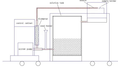
The erosion of X65 pipeline steel in simulated formation water was carried out in a homemade water-sand erosion loop system, which was composed of a control cabinet, screw pump, flow meter, sand feeder, solution tank, flowing jet and sample holder, as shown in Fig. 1. The flow velocity of water in the range of 5 to 20 m/s was adjusted by the rotation handle on the screw pump, and the sand concentration in water in the range of 0 to 0.2 wt.% was controlled by a sand feeder. The diameter of the flowing jet was 4 mm, and the distance and impingement angle between the jet and sample were fixed at 20 mm and 90°, respectively.

The weight of the samples was determined by using an electronic balance with an accuracy of 0.1 mg. The erosion test of X65 steel was carried out in simulated formation water with the flow velocities of 11, 14 and 17 m/s and sand concentrations of 0.05%, 0.10% and 0.20% (wt.%). The duration of the erosion test is 6 hours. After the erosion test, the samples were cleaned and weighed. The erosion rate of the X65 pipeline steel was calculated by using the following formula:

𝑣 =𝑚0−𝑚1

𝑆∙𝑡 (1)

where 𝑣 is the erosion rate in kg/(m2_{∙h); m}

0 is the mass weight before test (kg); m1 is the mass weight after the erosion test (kg); S is the exposed surface area of sample (m2_{); and t is the test duration (s). The} surface morphology of the test sample was observed by scanning electron microscopy (SEM).

To compare with the numerical simulation results, the erosion tests of X65 steel were also performed in simulated formation water without sand particles under different flow velocities.

Figure 1. Schematic diagram of the water-sand erosion loop system

Table 1. Chemical composition of X65 pipeline steel (wt. %)

C Si Mn P S Ni Cr

0.09 0.26 1.30 0.007 0.002 0.15 0.04

Table 2. Chemical composition of the testing solution (g/L)

NaCl KCl CaCl2 Na2SO4 MgCl2∙6H2O NaHCO3

3. NUMERICAL SIMULATION

3.1 Geometry and mesh models

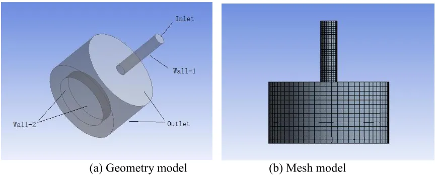
According to the above experimental design, the geometry model for flowing jet and sample was created, as shown in Fig. 2a. The geometry model is composed of three parts. One part is labelled as Inlet and Wall-1, which is used to simulate the flowing jet. The second part is Wall-2, which is used to simulate the test sample, and the third part is labelled as Outlet, which is used to simulate the outer domain around test sample. For numerical simulations, the computational domain was discretized by using the hex dominant mesh method. After automatic mesh based defeaturing, a grid with 13520 nodes and 15377 elements was generated, as shown in Fig. 2b.

3.2 Mathematical model

The testing solution was composed of a continuous phase (water) and a discrete phase (sand). During the simulation, it was assumed that water was incompressible flow, and there was no heat exchange between the water and sand particles. For the continuous phase, the steady state Reynolds averaged Navier-Stokes (RANS) equations were used for modelling the turbulence. The continuity and time averaged-momentum conservation equations (dropping the overbar on the mean velocity 𝑢̅) for the water phase are required to solve [14]:

(a) Geometry model (b) Mesh model

Figure 2. Geometry and mesh models of the erosion system under the impingement angle of 90°

Continuity equation:

𝜕𝜌 𝜕𝑡+

𝜕

𝜕𝑥𝑖(𝜌𝑢𝑖) = 0 (2) Momentum equation

𝜕

𝜕𝑡(𝜌𝑢𝑖) + 𝜕

𝜕𝑥𝑗(𝜌𝑢𝑖𝑢𝑗) = −

𝜕𝑝 𝜕𝑥𝑖+

𝜕 𝜕𝑥𝑗[𝜇 (

𝜕𝑢𝑖

𝜕𝑥𝑗+

𝜕𝑢𝑗

𝜕𝑥𝑖−

2 3𝛿𝑖𝑗

𝜕𝑢𝑙

𝜕𝑥𝑙)] +

𝜕

𝜕𝑥𝑗(−𝜌𝑢𝑖

′_𝑢 𝑗′

̅̅̅̅̅̅) (3)

where ρ is density, u is velocity, p is the static pressure, and μ is viscosity of the water phase. The additional term(−ρu_i′_u

j ′

shear stress transport (SST), which is based on a blending of k-ω and k-ε turbulence models, was used to express the turbulent fluid flow in the inner region of the boundary layer, as well as in the outer part of boundary layer, for a wide range of Reynolds numbers [15, 16]. The transport equations for the SST k-ω model had the following forms [14]:

𝜕

𝜕𝑡(𝜌𝑘) + 𝜕

𝜕𝑥𝑖(𝜌𝑘𝑢𝑖) =

𝜕 𝜕𝑥𝑗(𝛤𝑘

𝜕𝑘

𝜕𝑥𝑗) + 𝐺𝑘− 𝑌𝑘 (4)

𝜕

𝜕𝑡(𝜌𝜔) + 𝜕

𝜕𝑥𝑗(𝜌𝜔𝑢𝑗) =

𝜕 𝜕𝑥𝑗(𝛤𝜔

𝜕𝜔

𝜕𝑥𝑗) + 𝐺𝜔− 𝑌𝜔+ 𝐷𝜔 (5)

In these equations, the term Gk represented the production of the turbulence kinetic energy; Gω represented the generation of ω; Γk and Γω represented the effective diffusivity of k and ω, respectively; Yk and Yω represented the dissipation of k and ω, respectively, due to turbulence; and Dω represented the cross-diffusion term.

For the discrete phase, sand particles were tracked using the discrete phase model (DPM) in the Lagrangian frame of the reference where the particle trajectory was given as [10, 14]:

𝑑𝑥

𝑑𝑡 = 𝑢𝑝 (6)

The trajectory of a discrete phase particle could be predicted by integrating the force balance on the particle in ANSYS Fluent software. This force balance equated the particle inertia, with the forces acting on the particle, and could be written as [14]:

𝑑𝑢𝑝

𝑑𝑡 = 𝐹𝐷(𝑢 − 𝑢𝑝) +

g(𝜌𝑝−𝜌)

𝜌𝑝 + 𝐹𝑖 (7)

where Fi is an additional acceleration (force/unit particle mass) term, which included the virtual mass, Brownian force, Saffman’s lift force, and thermophoretic force [17]. The second term is the gravity force acting on the sand particle, which strongly depended on the water-sand density difference. 𝐹_𝐷(𝑢 − 𝑢_𝑝) is the drag force per unit particle mass, which depended on the water properties, particle geometry configuration, and sand-water velocity difference. FD is defined as:

𝐹𝐷 = 18𝜇 𝜌𝑝𝑑𝑝2

𝐶𝐷𝑅𝑒

24 (8)

where 𝑢 is the fluid phase velocity, 𝑢_𝑝 is the particle velocity, μ is the molecular viscosity of the fluid, ρ is the fluid density, 𝜌𝑝 is the density of the particle, and 𝑑𝑝 is the particle diameter. 𝑅𝑒 is the relative

Reynolds number, which is defined as: 𝑅_𝑒 =𝜌𝑑𝑝|𝑢𝑝−𝑢|

𝜇 (9)

The drag coefficient 𝐶_𝐷as a function of the particle Reynolds number was defined by: 𝐶𝐷 = 𝑎1+

𝑎2

𝑅𝑒+

𝑎3

𝑅𝑒2 (10)

where 𝑎₁, 𝑎₂, and 𝑎₃ were constants that were applied over various ranges of the Reynolds number given by Morsi and Alexander [18], which was suitable for spherical particles. In this study, the drag force was the dominant term. The additional acceleration term, Fi, was often much smaller than the drag force and could be neglected.

Particle erosion rates could be monitored at wall boundaries. The erosion rate was defined as [14, 19]:

𝑅𝑒𝑟𝑜𝑠𝑖𝑜𝑛= ∑

𝑚̇𝑝𝐶(𝑑𝑝)𝑓(𝛼)𝑣𝑏(𝑣)

𝐴𝑓𝑎𝑐𝑒

𝑁𝑝𝑎𝑟𝑡𝑖𝑐𝑙𝑒

𝑝=1 (11)

wall face, 𝑓(𝛼) was a function of impact angle, 𝑣 was the relative particle velocity, 𝑏(𝑣) was a function of the relative particle velocity, and 𝐴_{𝑓𝑎𝑐𝑒} was the area of the cell face at the wall. When the impact angle is 90°, the function of the impact angle is equal to 0.4 [11]. The velocity exponent and the diameter functions were set to 2.6 and 1.8*10-9_{, respectively [20].}

The type of solver was pressure-based, and the steady flow solver had been selected. In the parameter setting, the continuous phase was set to water, which was downloaded from the fluid database, and the density and viscosity of the water phase are ρ = 998.2 kg/m3 _{and μ = 1.003*10}-3 _kg/(m∙s), respectively. Similar to the sand used in erosion testing, the size and density of the particles was set to 300 μm and 2600 kg/m3_{, respectively. The particle trajectories were tracked using a discrete random} walk model [14, 21], which considered the effect of turbulent velocity fluctuations. The density of the wall face was set to 8030 kg/m3_{, which is similar to the density of the test sample. The boundary} condition of the inlet was set to velocity-inlet, which was suitable for incompressible flow. The outlet type was set to the outflow, which was generally used in a fully developed flow field. A convergence criterion of 1.0*10-5 _{was applied. Before calculation, the solution needed to be initialized.}

The ANSYS fluent 14.5 software was used to simulate the erosion behaviour of the X65 pipeline steel under different flow velocities and sand concentrations. After post processing of the numerical simulation, the flow path, pressure contour and erosion rate distribution were obtained.

4. RESULTS AND DISCUSSION

4.1 Effect of the flow velocity

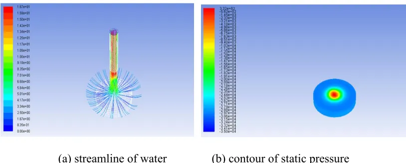
The streamline and static pressure contour of the erosion process under a flow velocity of 17 m/s and a sand concentration of 0.05% are shown in Fig. 3. It can be observed from Fig. 3 that the fully developed flow velocity occurs at the inside region of the outlet, which implies that the design length of the jet satisfies the requirement of a stable outlet flow.

(a) streamline of water (b) contour of static pressure

Figure 3. Streamline and static pressure contour on the sample surface under a flowing velocity of 17

In addition, the water phase diverges from the centre of the impact sample (Fig. 3a), which is in good agreement with the real water-sand erosion loop system in the experimental tests. From the centre to the periphery of the sample, the static pressure is continuously decreased (Fig. 3b). The maximum static pressure is located at the centre of the sample, which depends on the velocity of the water phase [10].

-0.010 -0.005 0.000 0.005 0.010

0.0 5.0x10-7 1.0x10-6 1.5x10-6 2.0x10-6 2.5x10-6 3.0x10-6 3.5x10-6 4.0x10-6

DPM Erosion ra

te ( kg/ (m 2*s )) Position (m)

-0.010 -0.005 0.000 0.005 0.010

0.0 5.0x10-7 1.0x10-6 1.5x10-6 2.0x10-6 2.5x10-6 3.0x10-6 3.5x10-6 4.0x10-6

DPM Erosion ra

te ( kg/ (m 2*s )) Position (m) (a) 11 m/s (b) 14 m/s

-0.010 -0.005 0.000 0.005 0.010

0.0 5.0x10-7 1.0x10-6 1.5x10-6 2.0x10-6 2.5x10-6 3.0x10-6 3.5x10-6 4.0x10-6

DPM Erosion ra

te ( kg/ (m 2*s )) Position (m) (c) 17 m/s

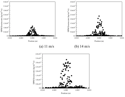
Figure 4. Distribution of the erosion rate of X65 steel by DPM numerical simulation under different

flow velocities with a sand concentration of 0.05%

Figure 5. SEM photograph of the sample surface exposed to a simulated formation water solution mixed

with 0.05 wt.% sands in a velocity of 14 m/s

X65 steel under different flow velocity can be obtained, which is shown in Table 3 and Fig. 6.

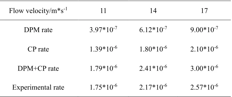
The erosion rate of X65 steel by the experimental water-sand erosion loop system was measured and is shown in Table 3 and Fig. 6. The erosion rate by the experimental method is clearly increased with the flow velocity and is slightly smaller than the DPM+CP rate. All of these results implied that there is a good consistency between the experimental rate and the simulation rate, and the numerical simulation method is appropriate for the erosion of X65 steel in simulated formation water. Similar results were also reported by Nguyen et al. [12], Aguirre and Walczak [25]. The different values of the inlet velocity were used in both numerical simulations and experiments to investigate the effect of the impact velocity on both the erosion rate and the surface evolution. Similarly, a mixture of water and sand was perpendicularly sprayed onto the surface of the test sample. It was clearly seen that a higher erosion rate was caused by the increasing of flow velocity under the same concentration of sand particles. It can be seen from Fig. 6 that the numerical results have the same trend as the experimental data. Both numerical simulations and experiments confirm that the erosion rate is a linear function of average inlet velocity. However, it can also be seen that the numerical simulation is larger than the experimental data. On the one hand, this can be explained by the fact that the sand particle shape factor is maintained constant throughout the entire simulation process, while the sand particles in our experiment become rounded in the erosion process due to the recycle use of sand particles. Moreover, the particle-particle interaction might also occur in the experiments, but this interaction is not considered in the simulations. On the other hand, the sand particles are treated as ideal points; therefore, the actual psychical presence of a finite-sized particle was not considered. This can lead to errors in predicting the particle-particle interaction as well as the particle rebounding from the sample surface, thus reducing the accuracy in predicting the erosion rate [32].

Table 3. Comparison of the erosion rate by numerical simulation and experimental methods under

different flow velocities

Flow velocity/m*s-1 _{11 14 17}

DPM rate 3.97*10-7 _6.12*10-7 _9.00*10-7

CP rate 1.39*10-6 _1.80*10-6 _2.10*10-6

10 12 14 16 18

0.0 5.0x10-7 1.0x10-6 1.5x10-6 2.0x10-6 2.5x10-6 3.0x10-6 3.5x10-6 4.0x10-6 Er osion ra te ( kg/ (m 2 *s ))

Flow velocity (m/s)

Experimental rate DPM rate CP rate DPM+CP rate

Figure 6. Erosion rate of X65 pipeline steel under different flow velocities

4.2 Effect of the sand concentration

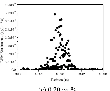
The distribution of the erosion rate of X65 pipeline steel by the discrete phase model under different sand concentrations in the flow velocity of 11 m/s is shown in Fig. 7. It can be seen from Fig. 7 that the maximum erosion rate is located in the centre of the sample and increased from 1.2*10-6 kg/m2_{∙s (sand concentration 0.05%) to 1.7*10}-6 _kg/m2_{∙s (0.10%) and 3.5*10}-6 _kg/m2_{∙s (sand} concentration 0.20%). Meanwhile, the radius of the eroded area increased from 0.0025 m (sand concentration 0.05%) to 0.005 m (sand concentration 0.20%). After the average, the erosion rates of steel under the sand concentrations 0.05%, 0.10% and 0.20% were 3.97*10-7_{, 7.9*10}-7 _{and 1.41*10}-6 _kg/(m2_∙s), respectively. These results are consistent with the research findings that were reported by other authors [33-36]. The sand particles could destroy the protective film on the material, thereby exposing the bare metal surface to the simulated formation water. The wear of the atoms on the metal surface accelerates with the increasing sand concentration. The impact, or abrasion, by sand particles is the dominant material removal mechanism [37,38].

-0.010 -0.005 0.000 0.005 0.010

0.0 5.0x10-7 1.0x10-6 1.5x10-6 2.0x10-6 2.5x10-6 3.0x10-6 3.5x10-6 4.0x10-6

DPM Erosion ra

te ( kg/ (m 2*s )) Position (m)

-0.010 -0.005 0.000 0.005 0.010

0.0 5.0x10-7 1.0x10-6 1.5x10-6 2.0x10-6 2.5x10-6 3.0x10-6 3.5x10-6 4.0x10-6

DPM Erosion ra

-0.010 -0.005 0.000 0.005 0.010

0.0

5.0x10-7

1.0x10-6

1.5x10-6

2.0x10-6

2.5x10-6

3.0x10-6

3.5x10-6

4.0x10-6

DPM Erosion ra

te

(

kg/

(m

2*s

))

Position (m) (c) 0.20 wt.%

Figure 7. Distribution of the erosion rate of X65 steel under different sand concentrations by numerical

simulation

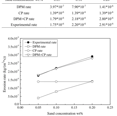
By considering that the erosion rate of the continuous phase (CP rate) under the flow velocity of 11 m/s is 1.39*10-6 _kg/m2_{∙s, as shown in Table 3, the erosion rates under the continuous phase and the} discrete phase are calculated and listed in Table 4. From Table 4, it can be seen that more erosion is caused by the discrete phase component (DPM rate) with the increasing sand concentration in the simulated formation water.

The erosion of X65 steel was tested in simulated formation water with different sand concentrations by using a water-sand erosion loop system, and the erosion rate was determined in Table 4 and Fig. 8. As shown in Table 4 and Fig. 8, the erosion rate of X65 steel clearly increased with the increasing sand concentrations, and the experimental erosion rate was nearly the same as the DPM+CP rate (Fig. 8) under different sand concentrations. It was observed that the numerical results also have the same trend as the experimental data. These results agree with previous observations [39].

Table 4. Comparison of the erosion rate by numerical simulation and experimental methods under

different sand concentrations

Sand concentration/ wt.% 0.05 0.10 0.20

DPM rate 3.97*10-7 _7.90*10-7 _1.41*10-6

CP rate 1.39*10-6 _1.39*10-6 _1.39*10-6

DPM+CP rate 1.79*10-6 _2.18*10-6 _2.80*10-6 Experimental rate 1.75*10-6 _2.20*10-6 _2.91*10-6

0.00 0.05 0.10 0.15 0.20 0.25 0.0

5.0x10-7 1.0x10-6 1.5x10-6 2.0x10-6 2.5x10-6 3.0x10-6 3.5x10-6 4.0x10-6

Er

osion ra

te

(

kg/

(m

2 *s

))

Sand concentration wt%

Experimental rate DPM rate

CP rate DPM+CP rate

Figure 8. Erosion rate of X65 pipeline steel under different sand concentrations

5. CONCLUSIONS

(1) With the increasing of flow velocity, the erosion rate of X65 pipeline steel in simulated formation water is clearly increased, and the erosion rates under the discrete phase and the continuous phase are both enhanced. Whereas the erosion rate of X65 pipeline steel, especially the erosion rate under the discrete phase, is increased rapidly with the increasing sand concentrations in simulated formation water.

ACKNOWLEDGEMENT

This work was jointly supported by National Natural Science Foundation of China (No. 51771133), the National Basic Research Program of China (No. 2014CB046801) and the Key Project of Tianjin Natural Science Foundation (No. 13JCZDJC29500).

References

1. I. Finnie, D. H. McFadden, Wear, 48(1978)181-190.

2. S. Turenne, M. Fiset, J. Masounave, Wear, 133(1989)95-106.

3. Y. I. Oka, H. Ohnogi, T. Hosokawa, M. Matsumura, Wear, 203(1997)573-579. 4. R. S. Lynn, K. K. Wong, H. M. I. Clark, Wear, 149(1991)55-71.

5. A. V. Levy, P. Chik, Wear, 89(1983)151-162.

6. A. H. Azimi, D. Z. Zhu, N. Rajaratnam, International Journal of Multiphase Flow, 40 (2012)19-37.

7. G. A. Zhang, L. Y. Xu, Y. F. Cheng, Corrosion Science, 51(2009)283-290. 8. L. Niu, Y. F. Cheng, Wear, 265(2008)367-374.

9. M. M. Stack, G. H. Abdulrahman, Tribology International, 43(2010)1268-1277. 10.H. S. Grewal, H. Singh, E. S. Yoon, Wear, 332(2015)1111-1119.

11.S. Shamshirband, A. Malvandi, A. Karimipour, M. Goodarzi, M. Afrand, D. Petković, M. Dahari, N. Mahmoodian, Powder Technology, 284(2015)336-343.

12.V. B. Nguyen, Q. B. Nguyen, Z. G. Liu, S. Wan, C. Y. H. Lim, Y. W. Zhang, Wear, 319(2014)96-109.

13.L. Zeng, G. A. Zhang, X. P. Guo, Corrosion Science, 85(2014)318-330.

14.ANSYS Fluent Theory Guide, ANSYS Inc., Southpoint, 275 Technology drive, Canonburg, PA 15317, USA.

15.V. B. Nguyen, H. J. Poh, Y. W. Zhang, Powder Technology, 256(2014)100-112. 16.F. R. Menter, AIAA journal, 32(1994)1598-1605.

17.P. G. T. Saffman, Journal of Fluid Mechanics, 22(1965)385-400.

18.S. A. Morsi, A. J. Alexander, Journal of Fluid Mechanics, 55(1972)193-208.

19.A. Amezcua, A. Gallegos-Muñoz, C. A. Romero, Z. Mazur-Czerwiec, R. Campos-Amezcua, Applied Thermal Engineering, 27(2007)2394-2403.

20.A. Gnanavelu, N. Kapur, A. Neville, J. F. Flores, N. Ghorbani, Wear, 271(2011)712-719. 21.A. Haider, O. Levenspiel, Powder Technology, 58(1989)63-70.

22.W. M. Zhao, C. Wang, T. M. Zhang, M. Yang, B. Han, A. Neville, Wear, 362-363(2016)39-52. 23. M. A. Islam, Z. N. Farhat, E. M. Ahmed, A. M. Alfantazi, Wear, 302(2013)1592-1601.

24. M. A. Islam, Z. N. Farhat, Tribology International, 68(2013)26-34.

25. J. Aguirre, M. Walczak, Tribology International, (2018), doi: 10.1016/j.triboint.2018.04.029. 26. S.S. Rajahram, T. J. Harvey, R. J. K. Wood, Tribology International, 43(2010)2072-2083. 27. J.Z. Yi, H.X. Hua, Z.B. Wang, Y.G. Zheng, Wear, 416-417(2018)62-71.

28. S. Zhou, M. M. Stack, R.C. Newman, Corrosion Science, 52(1996)934-946. 29. B. T. Lu, J. L. Luo, Journal of Physical Chemistry B, 110(2006)4217-4231.

30. J. H. Xie, A. T. Alpas, D. O. Northwood, Journal of Materials Science, 38.24(2003)4849-4856. 31. J. Jiang, Y. Xie, M. A. Islam, M. M. Stack, Journal of Bio- and Tribo-Corrosion, 3(2017)45. 32. A. Gnanavelu, N. Kapur, A. Neville, J. F. Flores, N. Ghorbani, Wear, 271(2011)712-719. 33. C.G. Telfer, M.M. Stack, B. D. Jana, Tribology International. 53 (2012)35-44.

34. H.X. Hu, Y.G. Zheng, Wear, 384(2017)95-105.

35. R. Elemurena, R. Evittsb, I. Oguochaa, G. Kennellb, R. Gerspacherb, A. Odeshia, Wear, 410-411 (2018)149-155.

37. Y. Wang, Z.Z. Xing, Q. Luo, A. Rahman, J. Jiao, S.J. Qu, Y.G. Zheng, J. Shen, Corrosion Science, 98(2015)339-353.

38. S.R. Li, Y. Zuo, P. Ju, Applied Surface Science, 331(2015)200-209.

39. V. B. Nguyen, Q. B. Nguyen, Y. W. Zhang, C. Y. H. Lim, B. C. Khoo, Wear, 348-349(2016)126-137.