New approaches of testing for financial market crisis and contagion

(1)

New Approaches of

Testing for Financial Market

Crisis and Contagion

Cody Yu-Ling Hsiao

A thesis submitted for the degree of

Doctor of Philosophy of

the Australian National University

April

:

2014

(2)

(3)

Declaration

This thesis comprises my original work, except for two chapters which are based on collaborations with Joshua Chan, Renee Fry-McKibbin, and Chrismin Tang. A version of Chapter 3 is a joint working paper with Renee Fry-McKibbin and Chrismin Tang, released in June 2013 as "Global Financial Crises" and is now forthcoming in Open Economics Review as "Contagion and Global Financial Crises: Lessons from Nine Crisis Episodes". A version of Chapter 5 is a joint working paper with Joshua Chan and Renee Fry-McKibbin, released in April 2013 as "A Regime Switching Skew-normal Model for Measuring Financial Crises and Contagion", GAMA Working Papers, 2013, No.15.

This thesis contains no material which has been accepted for the award of a degree or diploma in any university or institution .. To the best of my knowledge, it contains no material previously published or written by another person, except where due reference is made in the text of the thesis.

Cody Yu-Ling Hsiao

Centre for Applied Macroeconomic Analysis (CAMA) Crawford School of Public Policy

The Australian National University Canberra ACT 0200

(4)

Acknowledgments

First of all, I would like to express _{my sincere gratitude to my principal supervisor,} Renee Fty-McKibbin for giving me this great opportunity to work on this challenging project on financial market crisis and contagion. Her guidance, patience, continuous encouragement and financial support has been an invaluable contribution throughout the long journey of my PhD study and will always be appreciated. I am also deeply grateful for her many helpful suggestions that substantially improved the quality of research detailed in this thesis. Her generous support of conference attendance and academic visits have provided me with exceptional opportunities to interact with lead-ing experts in the field.

Likewise, my sincere _{gratitude goes to another of my supervisors, Joshua Chan}_, for his brilliant technical guidance and suggestions in study of Bayesian econometrics. In particular, he supervises _{me how to program the proposed models}_{in Mat}_lab ef-ficiently and gives me insightful suggestions on the improvement of financial models using Bayesian techniques. Without his involvement, the last chapter of this thesis will not have been possible finished. His encouragement and kindness will always be remembered.

I would like to thank Vance Martin for his valuable comments and suggestions for the fourth chapter of my thesis related to the size and power tests during his visit at Centre for Applied Macroeconomic Analysis (CAMA). I am also grateful to my thesis advisers Warwick McKibbin and Shaun Vahey, and many staff members and visiting scholars at the Australian National University (ANU), including Dirk Baur, Rob Breuning, Elliott Fan, Junsang Lee, Timothy Kam, Martine Mariotti, Juergen Meinecke, James Morley, Borek Puza, Sherrill Shaffer, Mathias Sinning, Michael Smith, Tom Smith, Rodney Strachan, Yong Song, Chrismin Tang and Jessie Xiaokang Wang for their teaching and providing me with assistance with my research.

I would like to extend my gratitude to my previous supervisor from National Chung Cheng University, Chia-Hung Sun, who guided my path to the PhD program at the ANU. I value greatly his continual support.

My research has benefited greatly from the comments of participants at the confer-ences I attended, namely: the 40th _{Australian Conference of}

(5)

24th Annual East Asian Seminar on Economics and the 2013 Australasian Meeting of the Econometric Society. I acknowledge the Crawford School of Public Policy and CAMA or financial support to attend conferences and workshops.

I would like to thank to my PhD schoolmates at the ANU, including Yiyong Cai, Patrick Carvalho, Thitima Chucherd, Syed Abul Hasan, Wei Jin, Sanghyeok Lee, Yin Liao, Andrew Liew, Larry Liu, Yingying Lu, Eugene Martin, Scott McCracken, Tomo-hito Okabe, Liyi Pan, Hyejin Park, Christopher Perks, Justin Wang, Wenjie Wei, Sum-ila Wanaguru, Varang Wiriyawit, Ben Wong, Sen Xue, Wenying Yao, and Guochang Zhao for their companionship and support. I also thank Megan Poore for the sug-gestions of a statement of my future research plan. Excellent administrative and IT support from Rossana Bastos-Pinto, Jay Giampieri, Damien Hughes, Han Lew, Su-sanna Pietrzak, Chris Treadwell, Robyn Walter and Hong Yu is kindly acknowledged.

I would like to thank my friends, Blair Alexander, Jamie Chang, Mia Chen, Ying-yi Chih, Michael Hsu, Cheng-Lei Hu, Eric Li, Aleck Lin, Melissa Lo, Guo Long, Elsa Su, and Tanabe Sugami for their invaluable friendship. Their friendship made my graduate life in Canberra particularly rich and provided wonderful memories that form the basis for our ongoing connection.

I would like to express my heartfelt thanks to my family and Vincent for their love and encouragement. They have always been my biggest motivation, enabling me to overcome obstacles that I encountered. I thank for your understanding and giving me the freedom _to pursue my research dream that has now finally become a reality.

(6)

Abstract

This thesis consists of four chapters _{that focus on the development of new statistical} frameworks or tests of financial market crisis and contagion.

A new test for financial market contagion _{based on changes in the fourth order} co-_{moments ( co-kurtosis and}_{co-volatility)} _{is proposed in Chapter 2 to identify the} propagation mechanism of shocks across international _{financial markets. This extends} the work of Fry et _{al. (2010) by deriving the}_co-kurtosis_and_co-volatilit_{y change} tests and fills a gap in the contagion literature that usually _{only focuses on} cross-market linkages between mean returns _{(correlation), and between mean returns}_and volatility (co-skewness). The proposed approach captures changes in various aspects of the asset return relationships such as cross-market mean and skewness (co-kurtosis) _as well as _{cross-market volatilities (co-volatility).}_{In an empirical}_{application involving the} global financial crisis _{of 2008-09, the results show that significant}_{contagion effects are} widespread from the US banking sector to global equity markets and banking sectors through either the co-kurtosis _{or the co-volatility channel.}

Chapter 3 analyses nine financial crises _{from Asia in 1997-98 to the recent European} debt crisis of 2010-13 to answer the question of whether the great recession is different to other crises in terms of a range of hypotheses regarding contagion transmission. This chapter examines financial contagion _{with a focus on the}_{correlation and} co-skewness change tests, and the proposed co-volatility change _{test developed in Chapter} 2 to capture changes _{in the various aspects of the}_asset _{return relationships. The} em_{pirical results indicate that the great recession}_and_{European debt}_{crisis are}_truly global financial crises. Linkages through financial channels are more likely _{to result in} crisis transmission than through trade, _{and crises beginning emerging}_{markets transmit} unexpecte_{dly, particularly to developed markets.}

(7)

that the joint tests identify various combinations of transmission channels during the three crises.

Chapter 5 introduces a new framework for testing for crisis and contagion using a regime switching skew-normal model (RSSN model). The RSSN model is built based on the regime switching model but with relaxation of the assumption of normality of the distribution which is assumed to be a multivariate skew-normal distribution. This new approach provides a more general framework for developing five types of crisis and contagion channels simultaneously. Measuring financial contagion within the RSSN model can solve several econometric problems faced in the contagion literature. These are i) market dependence is fully captured by simultaneously considering both second and third order co-moments of asset returns; ii) transmission channels are simultane-ously examined; iii) crisis and contagion are distinguished and individually modelled; iv) the market that a crisis originates is endogenous; and v) the timing of a crisis is endogenous. By applying the proposed model to equity markets during the great r e-cession using Bayesian model comparison techniques, the results generally show that crisis and contagion are pervasive across Europe and the US through the second and third moment channels during the great recession.

(8)

205 205 C.2 Derivation of Test Statistics for Joint Co-moments . 211 C.2.1 Correlation and Co-skewness₁₂Joint Test . . ₂₁₁ C.2.2 Correlation, Co-skewness_{12 ,}Co-skewness₂₁ Joint Test 214 C.2.3 Correlation, Co-skewness₁₂and Co-kurtosis₁₃Joint Test . 217 C.3 Forbes and Rigobon Adjusted Correlation Test . . . . . . . . . . 219

D Chapter 5 Appendix ₂₂₀

(13)

List of Tables

2.1 Descriptive statistics of the moments and co-moments of daily equity

returns for Hong Kong and the US . . . . . . . . 9

2.2 Simulation parameters of the moment and co-moment terms 47

2.3 Critical values for the test statistics . . . . . . . . . . . 48

2.4 Summary statistics of equity returns and banking sectors during the

non-crisis and crisis periods . . . . . . . . . . . . . . . 49

2.5 Statistics of the second and third order co-moments of equity returns

and banking sectors during the non-crisis and crisis periods . . . . . . . 50

2.6 Statistics of the fourth order co-moments of equity returns and banking

sectors during the non-crisis and crisis periods . . . . . . . . . . . . . . 51

2. 7 Testing for contagion based on changes in asymmetric dependence

dur-ing the global financial crisis of 2008-09 . . . . . . . . . . . . . . . . . . 52

2.8 Testing for contagion based on changes in extremal dependence during

the global financial crisis of 2008-09 . . . . . . . . . . . . . . . . . . . . 53

3.1 Crisis and non-crisis period dates . . . . . . . . . . . . . . . . . . . . . 62

3.2 The top 5 trading partners of crisis countries in the year prior to their

cr1s1s . . . . . . . . . . . . . . . . . . . . . . . . . . . . . 86

3.3 The top 5 portfolio investment partners of crisis countries prior to their

(14)

3.4 Contagion from the US equity market to recipie_{nt markets during the} LTCM and dot-com crises . . . . . . . . . . . . . . . . . . . . . . . 89 3.5 Contagion from the US equity market to recipient m_{arkets during the}

subprime and great recession crises . . . . . . . . . . . . . . . . . . 90 3.6 Contagion from the US equity market to recipient markets during the

European debt crisis . . . . . . . . . . . . . . . . . . . . . . . . . . 91 3. 7 Contagion from the US equity market to recipient markets during the

Asian and Russian crises . . . . . . . . . . . . . . . . . . . . . . 92 3.8 Contagion from the US equity market to recipient m_{arkets during th}_e

Brazilian and Argentinan crises . . . . . . . . . . . . ₉₃

4.1 Summary of single- _{and multiple-channel t}_ests_{of contagion} ₁₀₅ 4.2 Summary of restrictions on the parameters for the size and power tests 119 4.3 Size properties of single-channel and multiple-channel tests of contagion 120 4.4 The results of linear and asymmetric dependence j_{oint test}_{s of contagion}

during the three financial crises of 2007-12 . . . . . . . 121 4.5 The results of linear, asymmetric and extremal dependence joint tests

of contagion during the three financial crises of 2007-12 . . . 124

5.1 Evidence categories for the log of the Bayes Factor used for the model selection . . . . . . . . . . . . . . . . . . . . . . . . . . . . . 145 5.2 Summary of restrictions on the model parameters for tests of crisis and

contagion . . . . . . . . . . . . . . . . . . . . . . . . . . . . . 14 7 5.3 Summary statistics of the daily percentage equity returns over the period

(15)

B. l Summary of crisis dating in papers written on the Asian financial crisis 200

B.2 Summary of crisis dating in papers written on the Russian and LTCM

crises . . . . . . . . . . . . . . . . . . . . . . . . . . . . . . 201 B.3 Summary of crisis dating in papers written on the Brazilian, dot-com

and Argentinian crises . . . . . . . . . . . . . . . . . . 202 B.4 Summary of crisis dating in papers written on the subprime crisis and

(16)

List of Figures

2.1 Mean, volatility, skewness and kurtosis trade-offs. . . . . . . . . . . . . 20

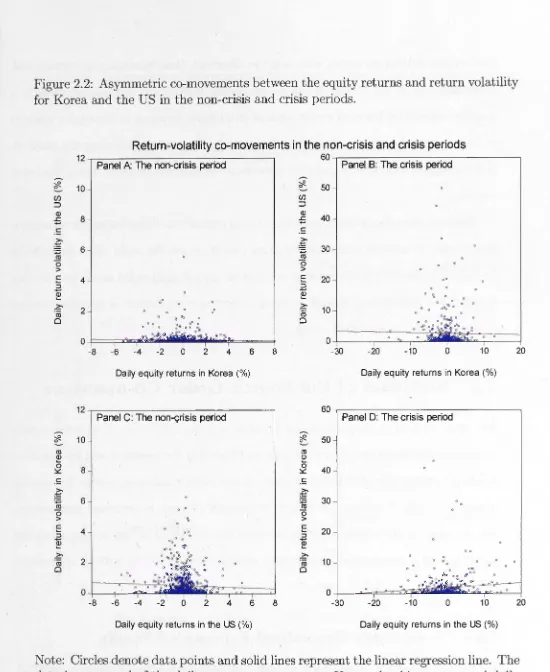
2.2 Asymmetric co-movements betw_ee_{n t}_h_{e e}_{quity returns}_a_{nd return vol}_at

il-ity for Korea and the US in the non-crisis and crisis periods. . . 22

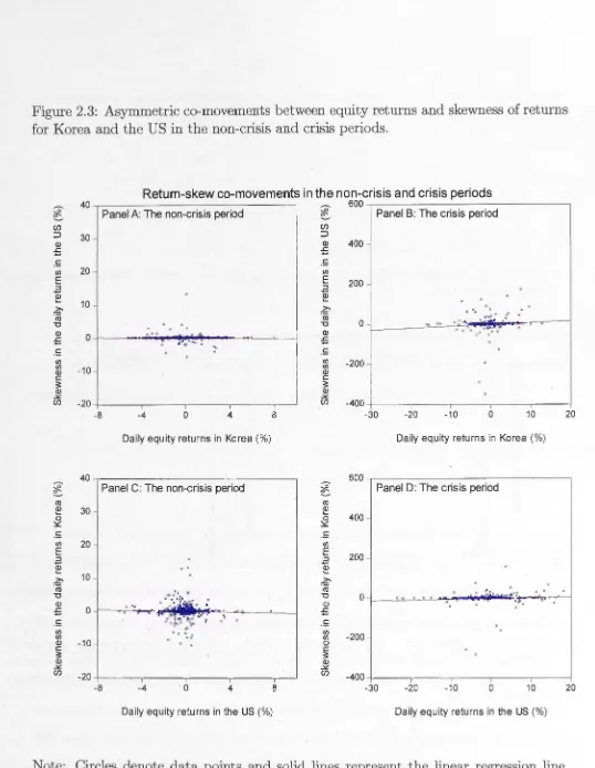
2.3 Asymmetric co-movements between equity returns _{and skewness of}

re-turns for Korea and the US in the non-crisis and crisis periods. . . 24

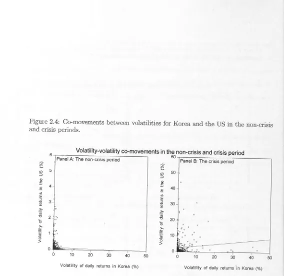
2.4 Co-movements between volatilities for Korea and the US in the non-crisis

and crisis periods. . . . . . . . . . . . . . . . . . . . . . . 25

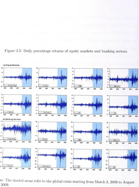
2.5 Daily _{percentage returns of}_e_quit_y_markets_a_{nd b}_a_nking_sectors_. ₃₉

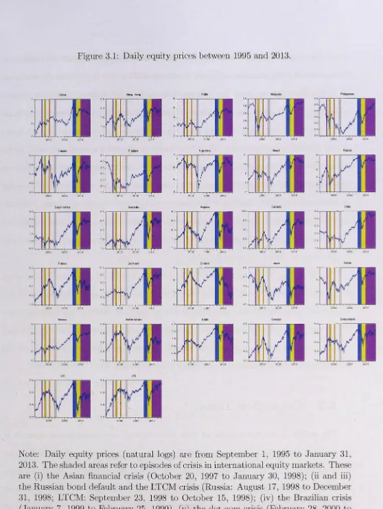
3.1 Daily equity prices between 1995 and 2013 .. . .

56

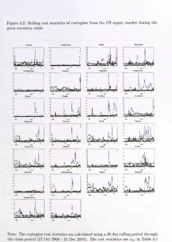
3.2 Rolling test statistics of contagion from the US equity market during

the great recession crisis. . . . . . . . . . . . . . . . . . . . . . . 7 4

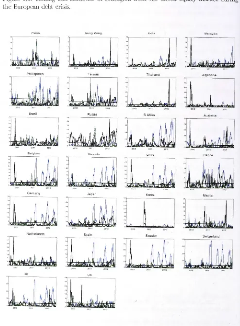
3.3 Rolling test statistics of contagion from the Greek equity market during

the European debt crisis. . . . . . . . . . . . . . . . . . . . . . . . . 75

3.4 Rolling test statistics of contagion from the Hong Kong equity market

during the Asian crisis. . . . . . . . . . . . . . . . . . . . . . . . . . 78

3.5 Percentage of markets affected by contagion for each crisis through trade

and finance linkages. . . . . _ . . . . . . . . . . . . . . . . . . . . . . 79

3.6 _{Percentage of markets}_a_ff_ecte_d_by_contag_{ion for}_eac_h_c_risis_throu_g_h

(17)

4.1 Simulated power functions of contagion statistics in experiment I. 111 4.2 Simulated power functions of contagion statistics in experiment II. 113 4.3 Simulated power functions of contagion statistics in experiment III. 115 4.4 Daily equity returns from 2005 to 2012. . . . . . . . . . . . . . 117

(18)

Chapter 1 Introduction

1.1 Motivation

"'\ ithin the last two _{decades, several financial}_crises_{have spread around}_the_{world and} affected both developing and de eloped countri_{es. The most prominent}_examples_of financial market crises o er this period include: the Asian Flu of 1997-98, the Russian Cold of 199 the LTC !I crisis of 1998 the Brazilian devaluation of 1999 the dot-com crisis of 2000 the Argentinian default crisis of 2001-02 the subprime mortgage cns1 of 2007-0 the great r cession crisis of 200 -09 _{and the recent European debt} cns1 of 2010-13. These crises aroused _{researchers interest in understanding increased} international equi market co-mo ement _{specificall around he period of crisis that} i chara erized b financial contagion. popular wa o think about he concep of on agion is through changes in he correla ion coefficien _{in roduced b Forbes and} Rigobon (2002) who gi e the defini ion of _{contagion as the change in he '"ransmission} mechani ms hat ak place during a cri is period compared o a non-crisis period. Al hough this i no he onl r wa · o hink about con agion thi _{me hod highlight}

Y ral challenging _{onom tri} _probl_ms _ha _ar _{in he use of echniqu}

for mea uring

(19)

First, the existence of a non-linear relationship between financial asset returns and

the statistical properties of asset return data, such as skewness and fat tails, suggests

that the correlation change tests of contagion may not be the only appropriate measure

of contagion. A range of alternative approaches of testing for contagion that go beyond

the linear approach include: the extreme value theory approach of Longin and Solnik

(2001), the outlier tests of Favero and Giavazzi (2002), the co-exceedance approach

of Bae et al. (2003), the latent factor approach of Dungey and Martin (2007), the

threshold tests of Pesaran and Pick (2007), and the co-skewness analysis of Fry et al.

(2010). Although non-linear approaches of financial market contagion have developed

in the literature, the extremal dependence ( co-kurtosis and co-volatility) tests of

finan-cial market contagion have been largely ignored. Extremal dependence ( co-kurtosis

and co-volatility) is another non-linear measure of market dependence that captures

more extreme co-movements than the linear dependence measures in the worst events

(Garcia and Tsafack, 2011). In an effort of fill this gap in the contagion literature,

test statistics for extremal dependence contagion linkages have been developed and are

detailed in Chapter 2. Three transmission channels of contagion are investigated in this

chapter: i) cross-market spillovers from the mean returns of the source market to return

skewness of the recipient market, ii) cross-market spillovers from the return skewness

of the source market to the mean returns of the recipient market, and iii) cross-market

spillovers between the return volatilities of the source market to the recipient market.

Second, as contagion tests are conditional on a state of nature, the dating of crisis

periods is an essential component of understanding contagion. However, the results

of contagion tests based on changes in correlation (Forbes and Rigobon, 2002) and

co-skewness (Fry et al., 2010) are sometimes not robust to the choice of crisis dates

(Dungey and Zhumabekova, 2001). In Chapter 3 of this thesis, instead of measuring

contagion using a fixed and arbitrary period of crisis, contagion is allowed to vary as

(20)

on a variety of platforms, and avoids the selection of _{the dating issue for the}_cr_isi_s

period. A range of studies have developed regime switching _{models for measuring}

financial market contagion _{to deal with the dating}_issu_e_{of the cr}_i_s_is_{period (Ang}_and

Bekaert, 2002; Pelletier, 2006; Gravelle et al., 2006; Billio et al., 2005; and Kasch

and _{Caporin, 2013). However, the regime}_switc_hin_g_{models of these papers}_ana

lyze

only the case of _{normality of the distribution, which for the}_case_{of financial market}

crisis and contagion, _{may ignore potentially important dimensions}_of_{financial market}

data _{and contagion aris}_in_g_{through non-linear dependence.} _In_{order to handle both}

the dating issues of the crisis period and _{the non-linear relationship between financial}

asset returns, a regime switching _{skew-normal model for measuring financial market}

crisis and contagion has been developed in Chapter 5.

Third, an extensive literature investigates the nature of return _{co-movements (Forbes}

and Rigobon, 2002; Fry et al., 2010), but these _{studies focus on the transmission} channels of market contagion onl_{y through either the corre}_l_ation_c_hann_e_l_{(Forbes and}

Rigobon, 2002) or higher _{order co-moments channel such as}_document_ed_in_the co-skewness tests of contagion (Fry et al., 2010). A major shortcoming of ignoring

ei-ther the correlation test of contagion or the higher _{order test of contagion could}

re-sult in _{omitting one of the possible}_{transmission channels such as cross-market mean}

returns spillovers, cross-market mean returns and return _{volatility spillovers,}

cross-market mean returns and return skewness spillovers, and cross-market return

volatili-ties spillovers. _{Chapters 4 and 5}_introduces_{several types of}_{multiple-channel}_{tests of} contagion in _{which the transmission channels of}_{financial market}_{crises can be id}_e_ntified jointly through the correlation, _{co-skewness and co-kurtosis channels.}

Fourth, the results _{of the correlation change test can be misleading}_{when a constant}

correlation coefficient is _{used as a proxy for}_{measuring financial}_contagion_rath_e_r_than using time-varying correlation (Baur, _{2003). Although Forbes}_and_Rigobon ₍₂₀₀₂₎

(21)

this test still suffers from problems arising from the homoskedasticity assumption. A

number of papers have documented that cross-market correlations are time-varying as

financial time series data are often characterized by time-varying heteroskedasticity

(Choe et al., 2012). In this thesis, a regime switching skew-normal model is developed

in Chapter 5 to allow for time-varying parameters including in the mean, volatility,

skewness, correlation and co-skewness for measuring financial crisis and contagion.

Finally, traditional methodologies developed to model contagion rely on identifying

the market that caused the crisis. It is not always possible to specify the trigger country during a financial crisis. A multivariate test for measuring financial contagion,

developed by Baur and Fry ( 2009), is one that avoids the difficulty of specifying the

asset market that precipitated the crisis. In Chapter 5 of this thesis, the proposed

regime switching skew-normal model endogenously determines whether a country is

deemed to be in crisis, rather than through an arbitrary choice.

This thesis develops several types of crisis and contagion tests which circumvent

several of the econometric challenges outlined. The proposed approaches are applied

to equity ma~kets and banking sectors during. nine financial crises ranging from Asia

in 1997-98 to the recent European debt crisis of 2010-13 ..

1.2 Review of the Results

The results of this thesis can be summarized· in several themes. The empirical results

indicate that the great recession (2008-09) and the European debt crisis (2010-13) can

be considered true global financial crises, based on single- and multiple-channel tests

of market crisis and contagion. Compared to trade linkages, financial linkages are

more likely to result in crises transmission during the great recession and emerging

market crises are transmitted unexpectedly, particularly to developed markets. The

(22)

multiple channels during _{the great recession.} _The_multiple-ch_{annel t}_{ests find more} evidence of crisis and _{contagion than the single-channel tests during}_{the great recession}_. Finally, the multiple-ch_annel_{tests of contagion are better than}_{the single-channel}

tests of contagion based on the size and power properties _{of the tests.}

1.3 _{Structure of the Thesis}

The key _{objectives of this thesis are consider}_e_{d in two}_{parts. The}_first

part consists of Chapters 2 and 3, which introduces _{several types of single-channel tests for}_fin_ancial market contagion. The second part, comprising _{Chapters 4}_an_{d 5,}_develops_several types of _{multiple-channel tests for}_financial_market_crisis_{and contagion.}

Chapter 2 introduc_{es a}new test of financial market contagion based on changes in the fourth order co-moments in the forms _{of co-kurtosis and co-volatility to identify t}_he propagation mechanism of shocks across international fin_ancial_{markets. The proposed} approach enables the analysis of changes in various aspects of the asset return rela-tionships such as cross-market mean and skewness ( co-_{kurtosis) as}_well_{as cross-market} volatilities (co-volatility) in order to fill a gap in the previous literature that only al-lows cross-market linkages _between_{mean returns}_{(correlation) and bet}

ween mean and

volatility (co-skewness). _{This new}_approac_{h is}_{applied to}_test_for_financial_contagion in equity markets and banking sectors that occurred during the global financial crisis of 2008-09. The results show that signifi_{cant contagi}_{on effects are widespread from}_the US banking sector to both global equity markets and banking sectors through these new channels.

(23)

correlation and co-skewness change tests and the proposed co-volatility change test

developed in Chapter 2 to capture changes in the various aspects of the asset return

relationships. Unlike the previous chapter which treats the period of crisis as fixed,

contagion is allowed to vary as the crisis unfolds in this chapter. This allows conclusions

to be drawn on the evolution and duration of contagion. The empirical results indicate

that the great recession and European debt crisis are true global financial crises.

Chapter 4 introduces a new class of multiple-channel tests of contagion in which

the transmission channels of financial market crises are identified jointly through the

correlation, co-skewness and co-kurtosis of the distribution of returns. Ignoring either

the correlation test or the higher order tests of contagion could result in the omission

of the possible transmission channels. The multiple-channel tests of contagion are

developed to allow the detection of transmission channels of contagion, not only through

the correlation channel, but also the higher order co-moment channels. The proposed

-multiple-channel tests in this chapter have the advantage over the existing

single-channel tests of contagion in the literature that they yield the correct size in small

samples as are typical of the crisis periods. Moreover, the multiple-channel tests of

contagion have the second highest power following the single-channel tests, as the data

generating process for the experiment contains the transmission channel of contagion

consistent with the single-channel test. The five multiple-channel tests of contagion

are applied to test for market contagion in equity markets during the three financial

crises from 2007-12. The results show that the joint tests identify various combinations

of transmission channels operating during the three crises.

Chapter 5 he RSS model for measuring financial crisis and contagion, which

al-lows a framework for developing a new class of single- and multiple-channel crisis and

con agion tests. This new approach provides a more general framework for developing

five types of single channel of crisis and contagion simultaneously. ore importantly,

(24)

contagion. _{Measuring financial}_contagion_{within the RSSN model}_can

solve several

econometric _{problems faced}_in_the_contagion_literature. _These_are

i) market depen-dence is fully captured by simultaneously considering _{both second and third order}

co-_{moments of asset returns;}_ii)_transmission_channels _{are simultaneously examined;}

iii) crisis and contagion _{are distinguished and}_individually_{modelled; iv) the market}

that a crisis _{originates is} _endogenous; _{and v) the timing}_{of a crisis}_is _endogenous.

By applying _{the proposed model to}_equity_{markets during the}_great

recession using Bayesian model comparison _{techniques, the results}_{generally show that}_crisis_and

con-tagion are pervasive across _{Europe and}_{the US through the second and}

third moments

channels during the great recession.

Chapter _{6 provides concluding}_remarks_{and suggestions}

for future research. Several statistical frameworks _{and tests of}_{financial market}_{crisis and contagion are developed in}

this thesis to circumvent several econometric problems _{addressed above.} _{The proposed}

approache_{s are applied to nine}_financial_crises_{ranging from Asia in 1997-98}

to the recent European debt crisis of 2010-13. For the future research, regime _{structure and}

alternative distributional assumptions such as _{heavy-tailed distributions in models}_of

contagion will be incorporated to develop new models for _{measuring financial market}

(25)

Chapter

2 A New Test of Financial Contagion

with Application to the US

Banking Sector

2.1 Introduction

The statistical properties of asset return data such as skewness arid fat tails would

suggest that the test for cross-marke~ contagion through changes in returns correlation

may not be the only appropriate approach for :measuring market contagion. This

chap-ter introduces three types of contagion tests to investigate three transmission channels

of contagion. .The three transmission channels are i) from mean returns of the source

market to return skewness of the recipient market; ii) from return skewness of the

source market to mean returns of the recipient ·market; and iii) from return volatilities of the source market to the recipient market.

. I

The contagious effect of financial crises has been of great concern to both academics

and policy makers because of its important consequences on the global economy that

specifically relate to monetary policy, risk management and asset pricing. Several major

(26)

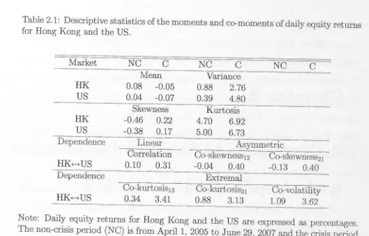
Table 2.1: Descriptive statistics of the moments _{and co-moments of}_daily_equity_returns

for Hong Kong and the US.

Market NC C NC C NC C

Mean Variance

HK 0.08 -0.05 0.88 2.76

us

0.04 -0.07 0.39 4.80

Skewness Kurtosis

HK -0.46 0.22 4.70 6.92

us

-0.38 0.17 5.00 6.73

Dependence _Linear _Asymmetric

Correlation _{Co-skewness12} _{Co-skewness21}

HKf---7 US _0.10 _0.31 _-0.04 _0.40 _-0.13 _0.40

Dependence _Extremal

Co-kurtosis13 _{Co-kurtosis31} _{Co-volatility}

HKf---7US _0.34 _3.41 _0.88 _3.13 _1.09 _3.62

Note: Daily equity returns for Hong Kong and the US are expressed as percentages.

The non-crisis _{period (NC)}_{is from}_April₁_,₂₀₀₅_to_Jun_e_{29, 2007}

and the crisis period

(C) is from March 3, 2008 to August 31, 2009. _Co-skewness1₂_{is measured}_in_terms_of

the returns of Hong Kong and squared returns of the US. _{Co-skewness21} is measured

in _{terms of the squared returns of}_{Hong Kong}_and_returns

of the US. Co-kurtosis13

is measured in terms of the returns of Hong Kong and cubed returns of the US.

Co-kurtosis31 is measured in _{terms of the cubed returns of}_{Hong Kong}_{and returns of}

the US. Co-volatility is measured in terms of the squared returns of Hong Kong and squared returns of the US.

features of financial crises are characterized in Table 2.1 using illustrative _{statistics of}

daily equity returns of Hong Kong and the _{US. Focussing first}_{on the statistics on}_a

univariate basis as shown in the top rows _{of the table, the average daily}_returns_of

equity indexes decrease from 0.08% to -0.05% in Hong Kong and from 0.04% to -0.07%

in the US during the global crisis of 2008-09 compared _{to the proceeding non-crisis}

period, while at _{the same time,}_daily_volatility_incr_eases_dramatically_{from 0.88}_% to 2. 76% in Hong Kong _{and from 0.39% to 4.80%}_in_{the US}_during_{the crisis}_{period. From}

the traditional _{mean-variance framework, a risk-averse}_inv_esto_r_{realizing a}

higher level

of the excess returns to compensate for a higher level of risk (Sharpe, 1964; Lintner,

[image:26.603.60.589.77.416.2]

(27)

The recent global crises remind investors that asset returns are driven by

asym-metric and fat-tailed distributions, suggesting that the Gaussian distribution is not an

appropriate distribution for modelling asset returns. This phenomenon is highlighted

in Table 2.1 demonstrated by negative skewness in the non-crisis period switching to

positive in the crisis period. It is evident that skewness preferences of investors are

subject to change in different regimes, as can be attributed to two types of effects.

The first is the risk return trade-off effect between the expected excess returns and

higher order moments. Lower asset returns occurring in a financial crisis are realized

in conjunction with positive skewness (Fry et al., 2010). The second is the volatility

skew and smile effect. Volatility skew is common in financial markets where stock

returns appear to be negatively correlated with return volatility (Black, 1976; Bekaert

and Wu, 2000). The bias phenomenon known as the volatility smile is often observed

in financial markets during a crisis period where the volatility-return co-movement

ex

-hibits an upward relation, resulting in positive skewness in the crisis period (Shleifer

and Vishny, 1997; Conrad et al., 2013).

Asset returns also typically yield leptokurtic behaviour (kurtosis is larger than

three) and kurtosis rises during turmoil periods ( see Table 2.1). Higher kurtosis of

returns is realized in conjunction with positive expected excess returns and return

skewness. Furthermore, the relatively lower kurtosis commonly displayed in the

non-crisis periods was documented theoretically by Brunnermeier and Pedersen (2008).

They found that speculators invest in securities with a positive average return and

negative skewness, giving rise to the low value of kurtosis. However, extreme events

resulted in speculators investing in securities with a negative average return and

nega-tive skewness, thus increasing kurtosis risk but provided a good hedge during the crisis

period.1

1

(28)

The dependence rows of the table shows how asset _{returns move relative to}_each

other over the same _{periods. Changes in the dependence}_{structure of asset}

returns in a crisis period are often observed _{in financial data}_and_{these changes}_{are the basis}

of different _{types of tests for}_contagion._{The contagion}_{tests are based on comparing the}

dependence structure _{of the asset returns in the non-crisis}_{and crisis}_{periods. The}

de-pendence rows of Table 2.1 shows three types _{of dependence structure}_{of asset returns:}

i) linear dependence, ii) asymmetric dependence and iii) extremal _{dependence during}

the non-crisis _{and crisis}_{periods. Each type of}_{market dependence models different} fea-tures of asset _{returns. The table shows}_that_{three types}_{of market dependence}

across asset returns are stronger in the crisis period than _{in the non-crisis period.}

In the contagion _{literature, linear dependence,}_{a correlation,}_is_commonly

used to measure financial contagion.2

Some researchers suggest that linear co-movement does

not fully capture market information since _{it is measured by}_{the equal weight of small}

and large returns _{(Embrechts et al.,}_2003). _Moreover,_corre_{lation is}

a linear measure of dependence that can be _{applied only when}_{investors display mean-variance}_preferences

, or in other words when returns follow a normal distribution.

In order to capture more market information _{on the asymmetry of the}

probabil-ity _{distribution of asset}_{returns rather}_{than the usual bivariate normal distribution,}

asymmetric dependence is captured in _{the co-skewness change tests of contagion}

in-troduced by Fry et al. (2010). _{Table 2.1 illustrates}_{that co-skewness (the relationship}

between the volatility in market i _{and the mean of the asset returns}_in_market

_j)

in equity returns between _{Hong Kong}_{and the}_US_switches_from_{negative to}_positive

during the financial _crisis_{of 2008-09.} _{The shift}_{from negative}

co-skewness to positive co-skewness _{during the financial crisis}_{comes from two potential}

effects which are i) the risk return trade-off effect and ii) _{the volatility skew and smile effect.} _{The co-skewness}

change tests of contagion _{developed by Fry}_{et al.} _{(2010) also reflects the fact that the}

2_Co_{ntagion i}_s_often

defined as a significant _{increase in}_correlat_ion_between_two_{markets during}

the

(29)

volatility-return correlation is not similar to the return-volatility correlation.3

Extremal dependence (co-kurtosis and co-volatility) is another non-linear measure

of market dependence and captures more extreme co-movements than the linear

depen-dence measures in the worst events. 4 _{Extremal dependence is measured by}_co-_kurtosis

( the relationship between the asset return in market i and return skewness in market

j)

and co-volatility (the relationship between the return volatility of markets i and

j).

The statistics of extremal dependence are highlighted in the bottom of Table 2.1

where co-kurtosis and co-volatility between equity returns in the Hong Kong and the

US increase during the global financial crisis that began in March 2008. This chapter

derives three tests of contagion based on changes in extremal dependence, which fills

a gap in the contagion literature.

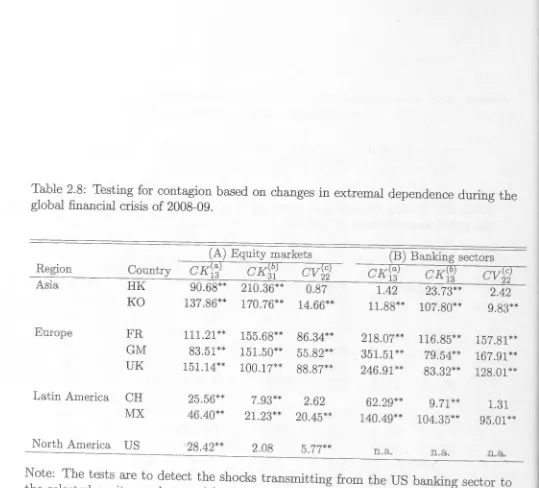
In this chapter, :financial contagion is defined as a significant cha:nge in extremal

dependence (as measured by the co-kurtosis and co-volatility) of two markets or

coun-tries between a non-crisis and a crisis period. This new approach is applied to test

for :financial contagion in equity markets· and banking sectors during the global

finan-cial crisis of ~008-09. The results of the tests show that significant contagion effects

are widespread from the US banking sector to global equity markets and from the US

banking sector to global banking sect.ors during the crisis period. More evidence of

con-. .

tagion is found through extremal dependence than through asymmetric dependence,

indicating tlie extremal dependence tests capture more co-movements during crises

than the asymmetric dependence tests in extreme events. In terms of the size test,

the results of simulation experiments show that the co-volatility change test presents

. .

a good approximation of the finite sample distribution regarding the relatively large

sample period of the non-crisis but the relatively short sample period of the crisis.

3_Bekaert_{and Wu (2000) examine causality}_from_a_{different perspective. The r}_et_urn_shocks_l_ea_d_to changes in conditional volatility, which arises from the leverage effect. However, the time-varying risk premium theory documents that return shocks are caused by changes in _conditional volatility.

4_{Garcia and}_Tsafack₍₂₀₁₁₎_{illustrate that}_{the tail}_dependence_{coefficient can be treated as the}

probability of the worst event occuring in one market given that the worst event occurs in another

(30)

The remaining sections of this chapter are organized as _{follows. Section 2.2 presents}

the traditional _{CAPM model with}_t_he _addition_of_higher_order

moments _and

co-moments in understanding the risk-return trade-off between the expected excess return

and higher order moments _{and co-moments}_._{Section 2.3 describes}_the

properties of a bivariate generalized exponential fami_{ly of}_{distributions with}_{asymmetry and}

leptokur-tosis, which _{provides th}_e_fram_e_{work for developing tests}

of co-skewness, co-kurtosis and co-volatili_{ty and tests of contagion}_{based on}_{changes in extremal}

dependence in Section 2.4. These tests are applied in Section 2.5 to investigate channels of contagion in equity markets and the banking sector _{during the financial}_{crisis of}_2008-09_._S_ection₂_.₆

offers conclusions.

2.2 Portfolio Choice

In standard _{theory of portfolio}_c_hoic_e, _inv_esto_rs_{achieve the optimal}

asset allocation

by maximizing the expected _{value of a}_utilit_y_fun_ct_ion

subject to the variance of the portfolio in the mean-variance framework (Sharpe, 1964; Lintner, 1965; and Black, 1972). As shown in Table _{2.1, the descriptive statistics}_e_mphasiz_e_the_import_ance_of modelling asymmetric and tail risks. Therefore, _{the traditional CAPM model}_with

higher _{order moments and}_co_-mom_ents_is_built_to_illu_strate

the risk return trade-off between _{expected excess}_{returns and}_hi_g_h_e_r

order moments and co-moments.

2.2.1 _{Portfolio Choice with Higher Order Moments}

Consider _{the standard}_utilit_y_fun_ct_ion_of_a_{n inv}_esto_r_all

ocating their portfolio across N risky assets _{to maximize their e}_nd_o_{f p}_e_riod_wealth_W

(31)

given the budget constraint:

N

ao

+Lai=

1.

i=l

The fraction of wealth allocated to the risk-free asset is a0 , and the fraction of wealth

allocated to the ith _risky_asset_is_ai._{The end of period wealth is}

N

W

=

ao (1

+

R1)

+

L ai (1

+

Ri) ,

i=l

(2.2)

· where Rf and Ri are the rates of return on the risk-free and risky assets respectively. Assume the distribution of returns of the investor's portfolio of risky assets to be

asymmetric and fat-tailed. In this case, the investor's utility function is constructed to

include higher order moments since the quadratic mean and variance do not completely

determine the distribution. Scott and Horvath (1980) show that investor preferences

for higher moments are essential for portfolio selection. The expected utility of the

return on investment W of the investor in this case is given by an infinite-order Taylor

series expansion around expected wealth:

00

u (q)

(w)

E [U (W)] =

L

.

,

E [

(w -

wf]

,

(2.3)

q=O q.

where the expected value of the end of period wealth is W E (W) and the q-th

derivative of U is U(q).

Equation (2.3) can be decomposed into the investor's risk preferences U (q)

(W)

and the q moments of the distribution

E

[

(W -

W)

q].

Scott and Horvath (1980) show that

under the assumption of positive marginal utility of wealth, a utility function exhibits

decreasing absolute risk aversion at all wealth levels with strict consistency for moment

preferences of U(q)

(W)

>

0 if q is odd and U(q)

(W)

<

0 if q is even.

(32)

utility function can be written as

E [U (W)]

u

_(w)

₊

u'

_(W)

_{E [}

_{(w -}

_w)]

₊

_1u"

_(W)

E [

(w -

W)

2]

+

~!

u"'

_{(W) E}

_[

_{(W - W)}

3]

+

:,

U( 4

)

(W) E

[

(w

-

W)

4

]

+

o(W), _(2.4)

where o(W) is _{the Taylor remainder.} _The_expected_r_etur_n_,

variance, skewness and kurtosis for the end of period return, Rp, _{are denoted by}

µp

E[Rp]

cr2

p

E

[

(

Rp - µP) 2] =

E [ (

W -

W)

2]

s3 _p

_{E [ (}

_{Rp -} _µP)3

] =

E [ (

W - W) 3]

k4 _p

_E

_{[ (}

_{Rp -} _µP

)4]

=

E

[

(W -

w)4]

,

where µP is the expected return on the portfolio defined as

where ai is _{the weight of the}_ith _asset

in the portfolio with ai

>

_{0 and}~ai

=

1.

i=O

(2.5)

(2.6)

The investor's equilibrium condition is solved by taking the first order conditions of the Lagrange of the utility function _{of wealth subject to the}_budget_{constraint as}

shown _{in Appendix A.}_l._The_{expected excess}_return_{on each}_risky

asset over the risk free rate is given by

E

(

D.) _

R

=

(BE

[

U

(

W

)

l

)

2.

(BE

[

U

(

W

)

l

)

₃

_(B

_E

_[

_U

(

W

)

l

)

_k4

.L Li J

B

2 a P

+

B 3

_s_P

+

_Bk4

P

(33)

where

a(iu (W)) (

a(zu" (W)))

(8E[U(W)])

-a°'i

80'2 - au(w) ,

p

-(

Ill )

(

8E[U(W)]) _ _ a°'i

8st - au(w) , aw

(

a(-pU( 4

) (W)))

(

8E[U(W)]) _ _ a°'i

8kt - au(w) ·

aw aw

(2.8)

Equation (2. 7) shows that the expected excess return on each risky asset contains two

elements: i) the portfolio risk premium involving higher order moments of volatility

(o-;), skewness

(s!)

and kurtosis (k; ); and ii) measures of the investor's risk preferences

for volatility (8E[U(W)J) skewness (8E[U(W)J) and kurtosis (8E[U(W)J)

80'~ ' 8s

t

.

8kt .

2.2.2 Portfolio Choice with Higher Order Co-moments

If an investor invests in two risky assets, N = 2, then the variance, skewness and

kurtosis of the end of period returns can be decomposed into

0"2

p E [ ( Rp -

µP)

2

]

(2.9)

E [

(t}

,

(14 - µ;) )']

aiE [(R1 - µ₁

)2]

+

a~E [(R2 - µ₂₎2]

+

2a1a2E [(R1 - µ_{1) (}R2 - µ₂)],

si

=

· ~

[

(~

a;(R,

-

µ,))']

(2.10)

a~ E [ (R1 - µ₁₎3]

+

a~E [ (R2 - µ₂

)3]

+

(34)

E [

(~

a,

(14

~

µ

,)

r]

_(2.11)

af E [(R1 - µ₁

)4]

+

atE [(R2 - _µ2

)4]

+

_{4aia2E [(R1 -} _µ₁

₎₃

₍_R₂_- _µ2)]

respectively.

Substituting equations (2.9) to (2.11) into equation (2.7) gives the _{expected excess}

return for asset i in terms of the second, third and fourth order moments and

co-moments. The co-moments include the correlation, co-skewness, co-kurtosis and

co-volatility as shown in the equations below and measure the dependence structures

between the asset returns.

E(R) - Rt 01E [(R1 - µ₁)2]

+

_{02E [(R2 -} _µ₂₎2_]

₊

_03E_[(_R1_- _µ_{i) (}_R₂_{- µ2)]}

+04E [(R1 - µ₁

)3]

+

0sE [(R2 - µ₂₎3]

+

05E [(R1 - µ₁₎2 (R2 - _µ2)]

+01E [(R1 - µ₁₎(R2 - µ₂₎2]

+

0sE [(R1 - µ₁

)4]

+

0gE [(R2 - _µ2

)4]

+010E [(R1 - µi)3 (R2 - µ_2)]

+

0uE [(R1 - µ₁) (R2 - µ2)3]

where

0 _ 2 ( 8E[U(W)]) 1 - al 8u2

p

0 ₂

=

a2 ( 8E[U(W)])

2 8u2

p

0

3 -_ ?n~LC , 1 L-<2 n, ( 8E[U(8u2 W)])

p

0 _ a3 (8E[U(W)]) 4 - 1 8s 3

p

e

-

_

3 (8E[U(W)]) 0 - a2 8s3

p

e

₆_-

_

3 _{a 1}2 _a2( 8E_a[U(W)]) 3 Sp

e _

₁_- 3 _a1a22(8E[U(W)])

8 Sp 3

0 _ 4 ( 8E[U(W)]) 8 - al 8k4

p

Equations (2.12) and (2.13) are valid for all i.

0 _ 4 ( 8E[U(W)]) 9 - a2 8k4

p

0 _ ₁₀_- 4 _a13 _a2(8E[U(W)])

8k4 p 0 _ _{ll -} 4 _a1a23 ( 8E[U(W)])

ak4 p 0 _ _{12 -} 6 _a1a22 2 (8E[U(W)])

ak4 •

p

(2.12)

(35)

Rewriting the expression in equation (2.12) for asset 1 gives:

01E _{[(R1 - µ1)}2]

+

02E _{[(R2 - µ2)}2]

+

03E [(R1 - µ1) (R2 - µ2)]

+04E _{[(R1 - µ1)}3]

+

05E [(R2 _{- µ2)}3]

+

05E [(R1 - _µ1

)2

(R2 - µ2)]

+01E _{[(R1 - µ1)}(R2 _{- µ2}

)2]

+

0sE [(R1 _{- µ1)4]}

+

0gE [(R2 - µ2)4]

+010E [(R1 _{- µ1}

)3

(R2 _{- µ2)]}

+

011E [(R1 - µ1) (R2 - µ2)3]

(2.14)

This equation decomposes the expected excess return for the risky asset 1 in terms

of risk prices and risk quantities. The risk prices (the 0i in equation (2.13)) are

ex-pressed in terms of the various risk aversion measures arising from the utility function of

the investor ( ( aE~~W)]), ( BE~tw)]) and ( aE~~w)])) and the shares of the asset in the

portfolio (ai)- The risk quantities contain the second moment terms of the variance and

covariance, the third moment terms of skewness (E _{[(R1 -} _µ1)3] and E [(R2 - _µ2)3])

and co-skewness (E [(R1 - _µ1

)2

(R2 - _µ2)] and E [(R1 - µ_{1) (R2}- _{µ 2)}2]), as well as

the fourth moment terms of kurtosis ( E [ ( R _{1 -} -µ_{1 )4]} and E [ ( _R2_{- µ2})4] ) , co-kurtosis

(E [(R1 _{- µ1)}3 (R2 _{- µ2)],}E [(R1 - _µ1)(R2 - _µ2)3]) and co-volatility (E [(R1 - _µ1)2 (R2 - _µ2

)2]).

2.2.3 Effects of Higher Order Moments on Risky Assets

To illustrate the properties of the expected excess return for risky asset 1 in

equa-tion (2.14) under the scenario of higher order co-moments, the risk-return trade-off

surfaces between the expected excess return, the variance, skewness and kurtosis, are

(36)

the parameters governing the simulation· are chosen as5

0.5, 02 = _{0. 7}, 03 = 2.0, 04 = -1.5, 05 = -1.5

06 -1.5, 07 = -1.5, 08 = 4.0, 09 = 4.0, 010 = 1.5

0n 1.5, 012 = 1.5,

with the values of co-moments given by

E [(_{R1 - µ 1}) (R2 - µ2)]

E [(R1 - _µ1)(R2 _{- µ2)}2]

E [(R1 - _µ1)3 (R2 - µ2)]

0.80, E _{[(R1 - µ1}

₎₂

(R2 _{- µ2)]}

=

0.00

0.00, E [(R1 - µ_{1 )}(R2 _{- µ 2}

)3]

=

1.47 1.46, E [(R1 - _µ1

)2

(R2 - _µ2)2]

=

2.20.

(2.15)

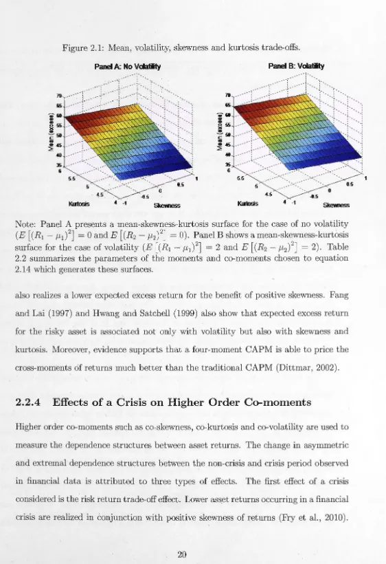
Panel A of _{Figure 2.1 presents}_the_{mean-skewness-kurtosis}_surface_for

a case where

there is no volatility (E _{[(R1 -} _µ1

_)2]

₌

0 and E _[(R2_{- µ2})2]

=

0) and panel B for a

case where there is volatility (E _[(R1_{- µ1)}2]

=

2 and E _{[(R2 -} _µ2)2]

=

2). Table 2.2

summarizes the simulation _{parameters for the}_{case o}_f_no_vo_l_at_ilit_{y (Pane}_l_A_of_Figure

2.1) _{and the case of vo}_l_at_ili_{ty (Panel}_B_of_{Figure 2.1). These parameters}

are chosen

from the data _{on which the emp}_iri_cal_results_are_based_in_{Section 2.5.2.}

Given any level of volatility in Panels A and B _{of Figure 2.1,}_there_is_a_positive

relationship between _{the expected excess}_return_and_{kurtosis while}_the_relationship

between skewness and kurtosis is _{negative. Comparing panel A with B}_of_Figure₂_.1_,_an

investor needs to be compensated _{for higher risk}_(volatility)_{with higher}_{expected excess}

returns. Given any level of kurtosis, there is a negative trade-off between expected

excess _{return and skewness.} _{These findings}_{suggest that an}_{investor requires}

a higher

expected excess return for taking more _{volatility and}_{kurtosis risks;}_{whereas, an}_investor

5

The parameters 04, ... , 0₇are restricted to have a _{negative sign due}_{to the assumption that a}

risk-averse investor has a _{utility function with decreasing absolute risk aversion,}_{while the other paramete}

(37)

[image:37.601.21.583.50.870.2]

Figure 2.1:. Mean, volatility, skewness and kurtosis trade-offs.

Panel B: Vala~

70

---1

65

1

0

Kmosis -4 -1

Skewness

70 65

l!i

6 ___ ,;_

5

-4_5 Kmosis

---,

0_5

0

-4 -1

Skewness

Note: Panel A presents a mean-skewness-kurtosis surface for the case of no volatility

(E

[(R

1 - µ1 )

2]

= 0 and E

[(R2 -

µ

2)

2]

= 0). Panel B shows a mean-skewness-kurtosis

surface for the case of volatility (E

[(R

1 - µ1 )

2 _]

₌

₂_and

E

[(R2 -

µ

₂₎

2 ]

=

2). Table 2.2 summarizes the parameters of the moments and co-moments chosen to equation

2.14 which generates these surfaces.

also realizes a lower expected excess return for the benefit of positive skewness. Fang

and Lai (1997) and Hwang and Satchell (1999) also show that expected excess return

for the risky asset is associated not only with volatility but also with skewness and

kurtosis. Moreover, evidence supports that a four-moment CAPM is able to price the

cross-moments of returns much better than the traditional CAPM (Dittmar, 2002).

2.2.4 Effects of a Crisis on Higher Order Co-moments

Higher order co-moments such as co-:-skewness, co-kurtosis and co-volatility are used to

measure the _. dependence structures between _. ~ asset returns. The . change in asymmetric

and extremal" dependence structures between t~e non-crisis and crisis period observed

in financial data is attributed to three types of effects. The first effect of a crisis

considered is the risk return trade-off effect. Lower asset returns occurring in a financial

New approaches of testing for financial market crisis and contagion