Single atoms in a standing-wave dipole trap
Wolfgang Alt,*Dominik Schrader, Stefan Kuhr, Martin Mu¨ller, Victor Gomer, and Dieter Meschede Institut fu¨r Angewandte Physik, Universita¨t Bonn, Wegelerstrasse 8, D-53115 Bonn, Germany
共Received 12 November 2002; published 19 March 2003兲
We trap a single cesium atom in a standing-wave optical dipole trap. Special experimental procedures, designed to work with single atoms, are used to measure the oscillation frequency and the atomic energy distribution in the dipole trap. These methods rely on unambiguously detecting presence or loss of the atom using its resonance fluorescence in the magneto-optical trap.
DOI: 10.1103/PhysRevA.67.033403 PACS number共s兲: 32.80.Lg, 32.80.Pj, 42.50.Vk
I. INTRODUCTION
In the last decade, optical dipole traps have become a standard tool for trapping ultracold samples of neutral atoms 共see Refs. 关1,2兴and references therein兲. In far-off-resonance traps关3兴atoms are trapped in a nearly conservative potential, where they exhibit a low spontaneous scattering rate leading to long coherence times up to several seconds 关4兴. These features, in combination with a great variety of possible trap designs and the ability to create time dependent trapping potentials, allow the study of classical and quantum chaos 关5兴, production and manipulation of Bose-Einstein conden-sates 关6兴, and investigations of ultracold atom mixtures 关7兴. These applications require the transfer of large numbers of cold atoms into the dipole trap关8兴.
In contrast, this work focuses on experiments with only a single or a few trapped atoms 关9,10兴. Our long-term objec-tive is the controlled manipulation of quantum states of in-dividual atoms. On the way to achieve this goal, we have recently demonstrated the possibility of manipulating the po-sition and the velocity of a single atom with high precision using a movable standing-wave optical potential关11,12兴.
To take full advantage of the available techniques, it is essential to access all trap parameters and to understand fun-damental effects such as lifetimes and heating effects. On the one hand, trapping of a few atoms avoids collisional loss and heating mechanisms associated with large numbers of atoms 关8兴. On the other hand, standard observation schemes such as time-of-flight methods based on direct imaging of an atomic cloud are not applicable.
Our methods rely on unambiguously detecting presence or loss of an atom using its resonance fluorescence from a magneto-optical trap 共MOT兲 关13兴. The ability to transfer an atom from the MOT into the dipole trap and back without any loss 关9兴 allows us to determine its survival probability after any intermediate experimental procedure in the dipole trap. Mastering this single-atom preparation and detection is the basis of the results presented in this paper.
In Sec. II, we briefly describe the standing-wave dipole trap and our experimental setup. In Sec. III, the relevant heating mechanisms for atoms in our trap are evaluated and put in relation with the observed lifetime. A measurement of the energy distribution of the atoms in the trap is presented in
Sec. IV, as well as the calculation of the adiabatic cooling involved. In Sec. V, we use the ability to manipulate the dipole potential in various ways to determine the axial oscil-lation frequency of the atoms, again using only one atom at a time. Finally, we summarize our results and point out future possibilities.
II. STANDING-WAVE DIPOLE TRAP
Our dipole trap consists of two counter-propagating Gaussian laser beams with equal intensities and parallel lin-ear polarizations. With their optical frequencies and ⫹⌬ (⌬Ⰶ) they produce a position- and time-dependent dipole potential
V共z,,t,U0兲⫽U0 w0 2
w2共z兲e
⫺22/w2(z)cos2
冉
⌬ 2 t⫺kz冊
.共1兲
Here, ⫽c/ is the optical wavelength, w2(z)⫽w02(1 ⫹z2/z0
2
) is the beam radius with waist w0, and Rayleigh length z0⫽w02/.
Both dipole trap laser beams are derived from a Nd:YAG 共Yttrium aluminum garnet兲laser (⫽1064 nm), which is far red detuned from the cesium D1- and D2-transitions共894 nm and 852 nm兲. In this case the maximum trap depth U0 is given by
U0⫽ប⌫ 2
P w02I0
⌫
⌬, 共2兲
where ⌫⫽2⫻5.2 MHz is the natural linewidth of the cesium D2-line, I0⫽1.1 mW/cm2 is the corresponding satu-ration intensity and P is the total power of both laser beams. Note that for red detunings (⌬⬍0), the dipole potential共1兲 provides three-dimensional confinement with a trap depth of 兩U0兩. For alkalis, the effective detuning⌬ is given by关1兴
1
⌬⫽
1 3
冉
1
⌬1⫹
2
⌬2
冊
, 共3兲where ⌬i is the detuning from the Di-line. Here,⌬⫽⫺2
⫻64 THz. The laser beam parameters are w0⫽30m, z0 ⫽2.7
⬙
mm with a total power of P⫽4 W, which yields a potential depth U0 of 1.3 mK.An atom of mass m trapped in such a standing-wave po-tential oscillates共in harmonic approximation兲 with frequen-cies
⍀z⫽2
冑
2U0m2, 共4兲
⍀rad⫽
冑
4U0mw02, 共5兲
in axial and radial directions, respectively. In our case ⍀z/2⫽380 kHz and⍀rad/2⫽3.1 kHz.
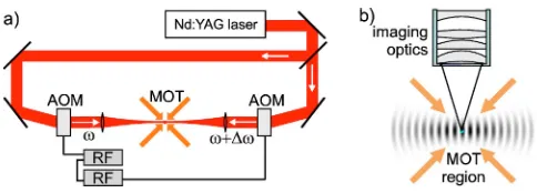
Figure 1 shows a schematic view of the experimental setup共see Ref.关12兴for more details兲. A magneto-optical trap with a high-magnetic-field gradient serves as a source of single cold atoms关9兴. The fluorescence light from the MOT is collected by imaging optics covering a solid angle of 0.02⫻4 关14兴 and is detected by an avalanche photodiode. From each atom in the MOT, we obtain up to 5⫻104 counts/s on a stray light background of only 2⫻104 s⫺1. This allows us to determine the number of trapped atoms within 10 ms.
These atoms can be transferred from the MOT into the dipole trap or back by operating both traps simultaneously for several 10 ms. When the focus of the dipole trap laser is carefully superimposed with the MOT, this transfer occurs without any loss of atoms关9,12兴.
An atom initially trapped in the stationary standing-wave dipole trap共laser beam frequency difference⌬⫽0) can be moved along the optical axis by changing⌬ which causes the potential wells to move at the velocity v⫽⌬/4. To control the frequency difference⌬, both dipole trap laser beams pass through acousto-optical modulators 共AOMs兲, which are set up in double-pass configuration to avoid angu-lar deviation of the beams. While both AOMs are driven with the same frequency AOM⫽2⫻100 MHz the standing-wave pattern is at rest and atoms can be loaded into the dipole trap. To accelerate them along the dipole trap axis one of the AOMs is driven by a phase-continuous linear fre-quency ramp. In a similar fashion, they can be decelerated and brought to a stop at a predetermined position along the standing wave 关11,12兴.
III. HEATING MECHANISMS AND LIFETIME
Without additional cooling, the lifetime of atoms in a di-pole trap is ultimately limited by heating. A fundamental source of heating in dipole traps is spontaneous scattering of trap laser photons. Due to large detuning of the trapping laser, the photon scattering rate at the maximum trapping laser intensity
Rs⬇
U0⌫
ប⌬ 共6兲
is only 14 s⫺1. Each photon adds on average one recoil en-ergy Er⫽(បk)2/2m on absorption and on spontaneous emis-sion. Therefore the energy E of an atom in the dipole trap potential increases as
具
E˙典
⫽2RsEr 关1兴.The above scattering rate yields a recoil heating rate of about
具
E˙典
⫽0.9K/s which is negligible in our experiment. Heating due to dipole force fluctuations 关15兴is at least four orders of magnitude smaller than the recoil heating.Technical heating can occur due to intensity fluctuations and pointing instabilities of the trapping laser beams as dis-cussed in detail in Ref. 关16兴. In the first case, fluctuations occurring at twice the trap oscillation frequency ⍀0 can parametrically drive the oscillatory atomic motion. For a spectral density of the relative intensity noise S(⍀) of the trapping laser and in harmonic approximation the energy in-creases exponentially according to Ref.关16兴
具
E˙典
⫽␥具
E典
with ␥⫽⍀0 22 S共2⍀0兲. 共7兲
Even for the free-running industrial laser used here with a relative intensity noise spectral power density of 3 ⫻10⫺11/Hz at 2⍀rad and 3⫻10⫺14/Hz at 2⍀z, the heating time constant is ⫽␥⫺1⬇300 s and 20 s, respectively.
In the case of pointing instability, shaking of the potential at the trap oscillation frequency increases the motional am-plitude. With S(⍀0) being the spectral density of the posi-tion fluctuaposi-tions the heating rate is given by关16兴
具
E˙典
⫽ 2 m⍀04
S共⍀0兲. 共8兲
In previous experiments with a running-wave dipole trap, using the same laser but more tightly focused to w0⫽5 m, we have observed lifetimes of one minute 关9兴. The smaller focus leads to a much higher radial oscillation frequency (⍀rad⬀w0⫺2). From the very strong dependency, Eq. 共8兲, of the heating rate on the oscillation frequency ⍀0, we infer that the pointing instabilities in radial direction are negligible in our current, less strongly focused dipole trap.
[image:2.612.53.295.55.142.2]All heating mechanisms described above, which are in-trinsic to any dipole trap, are not observable in this experi-ment and the measured trap lifetime of 25 s is limited by background gas collisions, see Fig. 2. However, in our ex-periments there is an additional technical noise due to fluc-tuations of the relative phase ⌬ between both AOM driv-ers. This phase noise is directly translated by the AOMs into FIG. 1. Experimental setup.共a兲MOT and dipole trap are
position fluctuations ⑀ of the dipole potential along the standing-wave axis
具
⑀2典
⫽具
⌬2典
/k2. The rms phase noise amplitude冑
具
⌬2典
⬇10⫺3rad has directly been measured by heterodyning both output signals of the AOM drivers.When this noise is evenly distributed over 1 MHz band-width and ⍀0⫽380 kHz, Eq. 共8兲 yields a heating rate of 4 mK/s. At higher oscillation amplitudes, the harmonic trap approximation presumed in Eq.共8兲breaks down and the os-cillation frequency goes to zero which slows down the heat-ing process.
We used a numerical simulation to obtain a realistic esti-mate of the lifetime in the anharmonic trapping potential 1. The one-dimensional equation of motion in the potential V(z,t)⫽U0cos2兵k关z⫹⑀(t)兴其is integrated numerically, starting with the atom at rest at z⫽0, until it leaves the potential well 兩z兩⬍/4. The potential is shaken with a Gaussian white noise⑀(t) with a bandwidth of 1 MHz and
冑
具
⌬2典
⬇10⫺3 rad. This results in an average lifetime of 2 s, in reasonable agreement with the experimental lifetime of about 3 s in the presence of phase noise共Fig. 2兲. The different heating rates are summarized in Table I.IV. ADIABATIC COOLING AND ENERGY DISTRIBUTION
The standard method of measuring the energy distribution of trapped atoms is the time-of-flight technique. There, the trap is switched off instantaneously and the velocity distribu-tion of the atoms in the trap is inferred from an image of their spatial distribution after ballistic expansion. This method cannot be used in our case because with only a single atom in the trap it would require very many repetitions to get useful statistics.
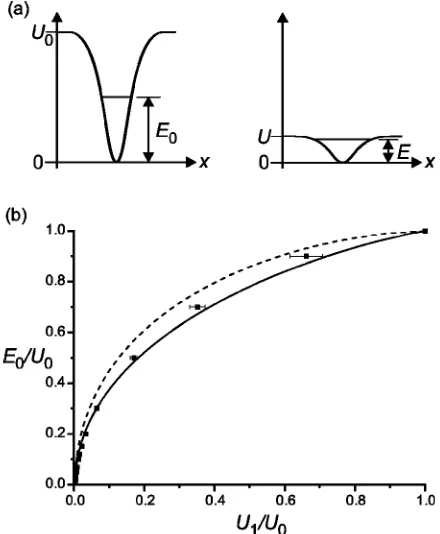
[image:3.612.65.284.56.220.2]A technique compatible with single atoms for measuring the energy distribution in the trap is to reduce the potential depth and to observe whether the atoms are lost. However, if this reduction of the potential is done quickly compared to the atomic oscillation period, the instantaneous kinetic en-ergy determines whether the atom escapes from the lowered potential. Thus, the loss probability depends on the phase of the oscillation at the moment the potential depth is reduced. If, in contrast, the trap depth is reduced slowly compared to the oscillation period, i.e., adiabatically, the trap depth U1 at which the atom escapes is a function of its total initial energy E0 only. By changing the potential depth from its initial value U0 to a value U, the energy of the atom is also changed from E0to E, due to adiabatic cooling, see Fig. 3共a兲. The atom escapes when the reduced trap depth U falls below E.
FIG. 2. Lifetime measurement with 共filled circles兲and without 共hollow circles兲phase noise at otherwise identical conditions. In the latter case, the decay is purely exponential and probably due to background gas collisions.
TABLE I. Heating mechanisms in the dipole trap and corre-sponding heating rates. For the resonant and parametric excitation, see Sec. V.
Heating effect Heating rate
Recoil heating 9⫻10⫺4mK/s共calc兲 Dipole force fluctuation heating 10⫺7mK/s共est兲 Laser intensity fluctuations共radial兲 4⫻10⫺3mK/s共calc兲 Laser intensity fluctuations共axial兲 6⫻10⫺2mK/s共calc兲 Laser pointing stability共radial兲 not observable AOM phase noise共axial兲 4 mK/s共calc兲
[image:3.612.328.548.58.325.2]0.4 mK/s共obs兲 Resonant excitation共axial兲 10 mK/s共obs兲 Parametric excitation共axial兲 10 mK/s共obs兲
FIG. 3. 共a兲 When the trap depth is adiabatically reduced from
U0to U, the energy of the atom inside the trap also decreases from E0to E.共b兲Atoms with energy E0in the original potential of depth U0 escape when the trap depth is reduced to U1. Solid line:
one-dimensional model, axial motion, V(x,U)⫽U关1⫺cos2(kx)兴. Dashed line: radial motion, V(x,U)⫽U关1⫺exp(⫺2x2/w0
2
[image:3.612.52.297.597.734.2]A. Theory
In a one-dimensional conservative potential V(x,U) of depth U⬎0, the action S⫽养p dx remains invariant under adiabatic variation 关17兴, where the integration is carried out over one oscillation period. If the potential is symmetric, V(⫺x,U)⫽V(x,U), the action can be written as
S共E,U兲⫽4
冕
0xmax
dx
冑
2m关E⫺V共x,U兲兴⫽const, 共9兲where E is the energy of the atom and xmax is the turning point of the oscillatory motion given by V(xmax,U)⫽E.
Equation 共9兲 allows us to calculate the initial atomic energy E0 from the measured trap depth U1, at which the atom is lost. Using the invariance of S we numerically solve S(E0,U0)⫽S(U1,U1) and show the resulting initial atomic energy E0 as a function of U1 for both axial and radial mo-tion in Fig. 3共b兲.
The invariance of S only holds for changes in U infini-tesimally slow compared to the oscillation frequency⍀, i.e., for 兩⍀˙ /⍀2兩→0. In order to optimally lower the potential within a limited time we keep⍀˙ /⍀2 constant. This requires ⍀(t)⬀1/t, which corresponds to, in harmonic approxima-tion, U(t)⬀1/t2. Smoothing the sudden transition from U(t)⫽U0to U(t)⬀1/t2at t⫽0 further improves the adiaba-ticity. In summary, the trap depth is reduced according to the function
U共t兲⫽
冦
U0 for t⭐0
U0
冉
1⫺ t24Tc2
冊
for 0⬍t⭐Tc
冑
2U0 Tc2
t2
for t⬎Tc
冑
2共10兲
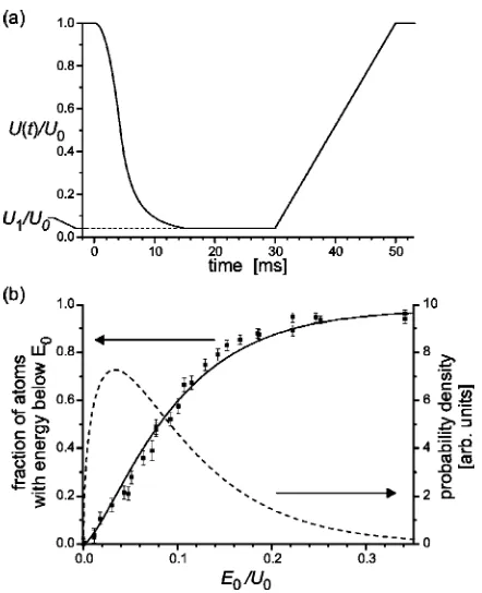
until it reaches U1, with a characteristic decay time of Tc ⫽3 ms. This keeps兩⍀˙rad/⍀rad2 兩⬍0.02. A graph of U(t) used in the experiment, including a waiting time of 15 ms and a ramp up back to U0, is shown in Fig. 4共a兲. Note that due to the anharmonicity of our potential ⍀→0 for E→U, which always violates the adiabaticity condition right before the atom leaves the trap. However, this energy region is rela-tively small and the corresponding error is of the order of ⫾2% of the initial energy E0.
The one-dimensional theory presented so far can only be applied to a separable three-dimensional potential V(x, y ,z) ⫽V1(x)⫹V2(y )⫹V3(z), where the equations of motion de-couple. The dipole trapping potential 共1兲 is not separable and, therefore, effectively couples the motional degrees of freedom. This leads to the possibility of a slow energy ex-change between them, the time scale of which can be long compared to the oscillation period. Hence, the lowering of the potential is not adiabatic with respect to this energy ex-change time. This raises the question whether the total atomic energy is responsible for the escape of the atom, or rather the motional energy in the direction of the preferred escape, i.e., along gravity.
To obtain quantitative information on the adiabatic cool-ing in three dimensions, classical atomic trajectories were calculated in a simplified time-varying potential, where 兩z兩 ⬍/4Ⰶz0 and, therefore, w(z) has been approximated by w0:
V共x, y ,z,t兲⫽U共t兲cos2共kz兲e⫺2(x2⫹y2)/w0 2
⫹mg y ; 共11兲
for U(t), see Eq. 共10兲 and Fig. 4共a兲. Atoms with a fixed energy E0but otherwise random starting coordinates are sub-jected to the simulated adiabatic lowering, in order to find out at which trap depth U1, or what range of trap depths, they escape.
The algorithm for determining random starting coordi-nates for a fixed initial energy E0 first randomly distributes E0 onto the three energies Ex,Ey,Ez. It then chooses
ran-dom phases for the oscillations in the three directions, to divide each of these energies into a potential and a kinetic fraction. These are used to calculate starting coordinates and velocities.
[image:4.612.328.549.54.326.2]The equations of motion in potential 共11兲are solved nu-merically, and atoms that depart more than 3w0 from the origin are counted as lost. For given values of the initial energy E0 and minimal potential depth U1 up to 120 trajec-tories are calculated to estimate the survival probability for FIG. 4. 共a兲Temporal variation of the potential depth for mea-surement of the energy distribution. Shown are the adiabatic reduc-tion to U1⫽0.04 U0according to Eq.共10兲, the waiting time and the
ramp up. 共b兲Cumulative energy distribution; measured fraction of the trapped atoms with energy below E0. The horizontal axis has
the atoms with a statistical error of ⫾0.05 . Then U1 is varied to find the value where the survival probability equals 0.5, see Fig. 3共b兲. Additionally, the 1 range of trap depths, over which the survival probability drops from 0.84 to 0.16, is shown as error bars. The three-dimensional simulations of the adiabatic cooling process agree qualitatively with the one-dimensional model. Due to the imperfect adiabaticity of the chosen U(t), Eq. 共10兲, atoms of one energy E0 do not escape at exactly one trap depth U1, but over a range of about ⫾10% of U1. This could be improved by making the lowering of the potential even slower.
B. Measurement of the energy distribution
To measure the energy distribution of the atoms, we trans-fer them from the MOT into the dipole trap before the trap depth is adiabatically reduced to U1 according to Eq.共10兲. This lowering of the potential takes between 10 ms and 51 ms for values of U1 between 0.082 U0 and 0.0036 U0, re-spectively. After waiting for 15 ms, the trap depth is ramped back up to U0 within 20 ms and the remaining atoms are transferred back into the MOT, see Fig. 4共a兲. The waiting time ensures that escaping atoms have traveled sufficiently far so that they are not accidentally recaptured.
We count the initial number of atoms by observing their fluorescence in the MOT for 50 ms before they are trans-ferred into the dipole trap. In the same manner, we infer the number of atoms that survived the above cooling process. We initially only load about five atoms into the MOT to ensure that on average no more than one atom occupies a potential well of the standing wave. For each value of U1, the above procedure was repeated 100 times to keep the er-ror, due to atom number statistics, below 3%. The change of the potential depth was realized by variation of the rf power of the AOM drivers, while the corresponding variation of both trap laser intensities was monitored by calibrated pho-todiodes.
The result of this measurement is the cumulative energy distribution, shown in Fig. 4共b兲. Note that the energy axis has been rescaled from the measured minimum potential depth U1 to the initial atomic energy E0 using the result of the three-dimensional trajectory simulations, shown in Fig. 3共b兲. Remember that in radial direction the dipole potential is modified by gravity 关12兴 such that theoretically at U1 ⫽0.0031U0, the effective potential depth is zero. It was found by extrapolation of the measured survival probability to zero that the effective potential depth in fact becomes zero at U1⫽0.0045U0, implying an actual trap depth slightly lower than theoretically expected 共see also Sec. V兲. This small discrepancy has approximately been taken into account by adding the difference of 0.0014U0 to the theoretical val-ues of U1, which corrects the influence of gravity for small values of U1 and is negligible at larger values.
The cumulative energy distribution of Fig. 4共b兲was fitted by the integral of a three-dimensional Boltzmann distribution p(E)⬀
冑
Eexp(⫺E/kT) 共shown as dashed line兲. This yields a temperature of kT⫽0.066U0. Using a trap depth of U0 ⫽1.3⫾0.3 mK we thus have T⫽0.09⫾0.02 mK. The error is due to the uncertainty in U0, indicated by the measuredoscillation frequency 共see Sec.V兲. This is slightly less than the Doppler temperature of TD⫽ប⌫/2⫽0.125 mK.
The resulting temperature of the atoms in the dipole trap is similar to the temperatures in our high-gradient MOT关18兴. The initial potential energy of an atom in the dipole trap depends on its position at the time the dipole trap is switched on. We, therefore, conclude that the MOT effectively cools the atoms into the dipole trap to about TD.
V. AXIAL OSCILLATION FREQUENCY
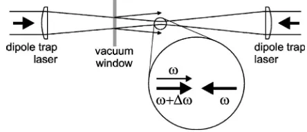
The axial oscillation frequency⍀zwas measured by reso-nant and parametric excitation of the oscillatory motion of a single atom in the dipole trap, exploiting the following fea-ture of our experimental setup: One of the dipole trapping laser beams passes through the window of our glass cell, which reflects about 4% of the incident power per surface. After divergent expansion, this third beam interferes with the two main laser beams and thus slightly changes amplitude and phase of their interference pattern 共see Fig. 5兲. When atoms are transported by mutually detuning the trapping beams by⌬ 共see Sec. II兲, both phase and amplitude of the trapping potential are modulated at that frequency. On reso-nance with⍀z, this excites the oscillation of the transported
atoms, which is, in turn, used here for determining ⍀z. In the atomic frame of reference moving with a velocity
v⫽ ⌬/4 the total electric field is
E共z,t兲⬀2 cos共t兲cos共kz兲⫹cos关共⫺⌬兲t⫺k
⬘
z兴, 共12兲where denotes the amplitude of the reflected beam in units of the incident beam amplitude. It can be shown that the leading terms of the resulting dipole potential forⰆ1 and k
⬘
⬇k are given byU共z,t兲⫽U0兵cos2共kz兲关1⫹cos共⌬t兲兴
⫺cos共kz兲sin共kz兲sin共⌬t兲其. 共13兲
The corresponding equation of motion around the equilib-rium position z⫽0 共assuming kzⰆ1) becomes
z¨⫹⍀z2关1⫹cos共⌬t兲兴z⫽⫺⍀z 2
2ksin共⌬t兲. 共14兲
[image:5.612.325.547.59.155.2]for⌬⫽2⍀zdue to the modulation of⍀z关17兴. This leads to heating of the atoms during transportation at mutual detun-ings of the laser beams near these two values.
This resonant heating effect is used for measuring the axial oscillation frequency ⍀z of the atom by keeping ⌬ constant for some time and by observing an increase of the oscillation amplitude. Since the standing-wave pattern of the dipole trap moves with a velocityv⫽⌬/4, we have to accelerate and decelerate the atom at the beginning and at the end, respectively, by suitable short frequency ramps. Finally, the displaced atom has to be brought back to the position of the MOT by a similar transport in the opposite direction.
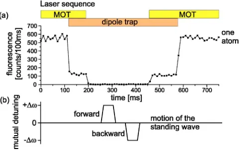
[image:6.612.55.296.58.212.2]The corresponding measurement sequence is shown in Fig. 6. Initially, a single atom is loaded from the MOT into the dipole trap. The detuning⌬is ramped up quickly, then kept at a constant value to expose the atom to the resonant heating and finally, it is ramped back down. We limit the total transportation distance to 2 mm because further away from the focus the trap depth, and thus ⍀z, decreases con-siderably.
Due to the anharmonicity of the trapping potential, reso-nant heating does not neccessarily lead to a loss of atoms. To decide whether an atom has been resonantly heated or not, we reduce the depth of the dipole trap in order to lose heated atoms. This is done adiabatically, as described in Sec. IV. We reduce the trap depth during 10 ms to 10% of its initial value. The reduction has been optimized to keep the atoms trapped most of the time in the absence of resonant heating, but to lose a substantial fraction of resonantly heated atoms. After waiting for 5 ms, the potential is ramped back up and any remaining atoms are recaptured into the MOT. The average survival probability is shown in Fig. 7, where we did about 100 shots with one atom for each value of⌬. The clearly visible dips at ⌬/2⫽330⫾5 kHz and ⌬/2⫽660 ⫾15 kHz correspond to direct and parametric resonance.
The measured axial oscillation frequency agrees
reason-ably well with the theoretical expectation of ⍀z/2 ⫽380 kHz. The discrepancy could be caused by any loss of trapping laser intensity at the focus, e.g., due to wavefront aberrations, or by reduced interference contrast, e.g. due to imperfect overlap of the two counterpropagating beams or not perfectly matched polarizations. Assuming 100% inter-ference contrast, we deduce a trap depth of U0⫽1.0 mK from the measurement.
We can estimate the energy gained during the resonant excitation as follows. During the adiabatic lowering of the trap depth to 0.1U0 all atoms with E0⬎0.35U0are lost关Fig. 3共b兲兴, leading to a survival probability of 90% off resonance. From the cumulative energy distribution 关Fig. 4共b兲兴, we see that the survival probability of 60% observed on resonance corresponds to a loss of atoms with E0⬎0.1U0. These atoms must have gained an energy of 0.25U0 during the resonant excitation period of 20 ms, yielding a time-averaged heating rate of about 16 mK/s. In the same way, a parametric heating rate of about 13 mK/s is found.
The same resonant excitation effect considered here causes a decrease of the transportation efficiency for certain values of the acceleration as observed in Ref. 关12兴. These previous investigations showed that the transportation effi-ciency remains nearly constant (⬎95%) until the accelera-tion exceeds a value of 105 m/s2. However, for certain in-termediate values of the acceleration values, at which the detuning ⌬ matched the oscillation frequency ⍀z, we ob-served a reduction of the transportation efficiency to 75%, which we attribute to the resonant excitation discussed above.
VI. CONCLUSIONS AND OUTLOOK
The temperature as well as the energy distribution of the atoms in the dipole trap were measured with procedures de-signed to work with single atoms. These procedures rely on our ability to transfer single atoms between MOT and dipole trap with high efficiency and to unambiguously detect their presence or loss. The axial oscillation frequency was deter-FIG. 6. 共a兲Measurement procedure for the axial oscillation
fre-quency. A single atom is loaded from the MOT into the dipole trap. During simultaneous operation of both traps, fluorescence of the atoms is reduced due to the light shift. Inside the dipole trap the atom is moved and then brought back again to the original position. Finally, the presence of the atom is detected by recapturing it back into the MOT. 共b兲 Mutual detuning of the two dipole trapping beams during the transport共not to scale兲.
[image:6.612.328.547.61.215.2]mined using controlled transportation of the atom.
The measured temperature of 0.09 mK and oscillation fre-quency of 330 kHz indicate a mean oscillatory quantum number of 6. Together with state selective detection关9兴this is a good starting point for Raman cooling of a single atom to the oscillatory ground state 关19兴. This will enable us to
more precisely control the internal and external degrees of freedom of single neutral atoms.
ACKNOWLEDGMENTS
We have received support from the Deutsche Forschungs-gemeinschaft and the state of Nordrhein-Westfalen.
关1兴R. Grimm, M. Weidemu¨ller, and Y.B. Ovchinnikov, Adv. At., Mol., Opt. Phys. 42, 95共2000兲.
关2兴V.I. Balykin, V.G. Minogin, and V.S. Letokhov, Rep. Prog. Phys. 63, 1429共2000兲.
关3兴J.D. Miller, R.A. Cline, and D.J. Heinzen, Phys. Rev. A 47, R4567共1993兲.
关4兴N. Davidson, H.J. Lee, C.S. Adams, M. Kasevich, and S. Chu, Phys. Rev. Lett. 74, 1311共1995兲.
关5兴V. Milner, J.L. Hanssen, W.C. Campbell, and M.G. Raizen, Phys. Rev. Lett. 86, 1514共2001兲; N. Friedman, A. Kaplan, D. Carasso, and N. Davidson, ibid. 86, 1518共2001兲.
关6兴D.M. Stamper-Kurn, M.R. Andrews, A.P. Chikkatur, S. Inouye, H.-J. Miesner, J. Stenger, and W. Ketterle, Phys. Rev. Lett. 80, 2027共1998兲; M. Barrett, J. Sauer, and M.S. Chapman, ibid. 87, 010404 共2001兲; T.L. Gustavson, A.P. Chikkatur, A.E. Lean-hardt, A. Go¨rlitz, S. Gupta, D.E. Pritchard, and W. Ketterle, ibid. 88, 020401共2002兲.
关7兴A. Mosk, S. Kraft, M. Mudrich, K. Singer, W. Wohlleben, R. Grimm, and M. Weidemu¨ller, Appl. Phys. B: Lasers Opt. 73, 791共2001兲.
关8兴S.J.M. Kuppens, K.L. Corwin, K.W. Miller, T.E. Chupp, and C.E. Wieman, Phys. Rev. A 62, 013406共2000兲.
关9兴D. Frese, B. Ueberholz, S. Kuhr, W. Alt, D. Schrader, V. Go-mer, and D. Meschede, Phys. Rev. Lett. 85, 3777共2000兲. 关10兴N. Schlosser, G. Reymond, I. Protsenko, and P. Grangier,
Nature共London兲411, 1024共2001兲.
关11兴S. Kuhr, W. Alt, D. Schrader, M. Mu¨ller, V. Gomer, and D. Meschede, Science 293, 278共2001兲.
关12兴D. Schrader, S. Kuhr, W. Alt, M. Mu¨ller, V. Gomer, and D. Meschede, Appl. Phys. B: Lasers Opt. 73, 819共2001兲. 关13兴Z. Hu and H.J. Kimble, Opt. Lett. 19, 1888 共1994兲; F.
Rus-chewitz, D. Bettermann, J.L. Peng, and W. Ertmer, Europhys. Lett. 34, 651共1996兲; D. Haubrich, H. Schadwinkel, F. Strauch, B. Ueberholz, R. Wynands, and D. Meschede, ibid. 34, 663 共1996兲.
关14兴W. Alt, Optik共Stuttgart兲113, 142共2002兲.
关15兴J. Dalibard and C. Cohen-Tannoudji, J. Opt. Soc. Am. B 2, 1707共1985兲.
关16兴T.A. Savard, K.M. O’Hara, and J.E. Thomas, Phys. Rev. A 56, R1095 共1997兲; M.E. Gehm, K.M. O’Hara, T.A. Savard, and J.E. Thomas, ibid. 58, 3914共1998兲.
关17兴L.D. Landau and E.M. Lifschitz, Mechanics共Pergamon, New York, 1976兲.
关18兴A. Ho¨pe, D. Haubrich, G. Mu¨ller, W.G. Kaenders, and D. Meschede, Europhys. Lett. 22, 669共1993兲.