Developing an Individual-level Geodemographic Classification

Developing an Individual-level

Geodemographic Classification

Luke Burns1&Linda See2&Alison Heppenstall1 & Mark Birkin1

Received: 10 March 2017 / Accepted: 18 August 2017 / Published online: 31 August 2017

#The Author(s) 2017. This article is an open access publication

Abstract Geodemographics is a spatially explicit classification of socio-economic data, which can be used to describe and analyse individuals by where they live. Geodemographic information is used by the public sector for planning and resource allocation but it also has considerable use within commercial sector applications. Early geodemographic systems, such as the UK’s ACORN (A Classification of Residential Neighbourhoods), used only area-based census data, but more recent systems have added supplementary layers of information, e.g. credit details and survey data, to provide better discrimination between classes. Although much more data has now become available, geodemographic systems are still fundamentally built from area-based census information. This is partly because privacy laws require release of census data at an aggregate level but mostly because much of the research remains proprietary. Household level classifications do exist but they are often based on regressions between area and household data sets. This paper presents a different approach for creating a geodemographic classification at the individual level using only census data. A generic framework is presented, which classifies data from the UK Census Small Area Microdata and then allocates the resulting clusters to a synthetic population created via microsimulation. The framework is then applied to the creation of an individual-based system for the city of Leeds, demonstrated using data from the 2001 census, and is further validated using individual and household survey data from the British Household Panel Survey.

Keywords Geodemographics . Small area microdata . Individual . Census . Classification DOI 10.1007/s12061-017-9233-7

* Luke Burns

L.P.Burns@leeds.ac.uk

1 _{School of Geography, University of Leeds, Woodhouse Lane, Leeds LS2 9JT, UK} 2

Introduction

Geodemographics is widely defined as the analysis of people based on where they live. It is concerned with segmenting the population into homogeneous groups based on a range of characteristics to enable the profiling of neighbourhood areas for commercial and public service planning applications (Longley2017). In the UK, the concept can be dated back to the 1970s and evolved from coarse scale census-based classifications to systems nowadays that make use of a myriad of individual and lifestyle data (Harris et al.2005). However, the notion of area classification is much older and has been around since the late nineteenth century with the work of Charles Booth (1889).

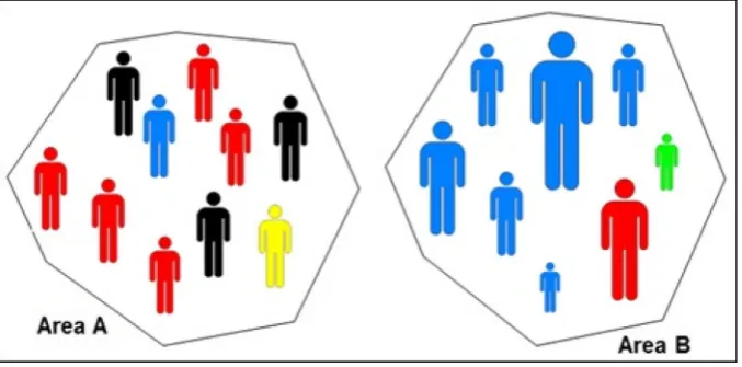
Commercial systems in the UK typically operate at postcode level (Petersen et al. 2011) with an average population of forty residents across each of the 1.75 million postcodes in the country (ONS2014). Other countries use differing levels of granularity but many remain restricted to areal units. However, the use of areal units creates spatial aggregation problems. Geodemographic classifications assume that each class is largely homogeneous based on the premise that "birds of a feather flock together"(Harris et al. 2005, p.16); hence people with similar traits tend to gravitate to similar locations. Whilst application-specific geodemographic systems such as those in health (Abbas et al.2009), crime (Ashby and Longley2005) and education (Singleton and Longley 2009) use carefully selected inputs, many of the commercial general-purpose systems include huge arrays of inputs designed to describe a range of lifestyle, behavioural and socioeconomic conditions. As more variables are added–both census/socioeconomic (e.g. age and housing type) and lifestyle/behaviour (e.g. expenditure and leisure activities),there is an increase in the prospective ambiguity as demonstrated in Fig.1. Two hypothetical areas exist: Area A and Area B (Fig.1). If Area A was statistically assessed independently and clustered into a crisp‘best fit’grouping based only on the shading of the individuals, this area would be assigned to a‘red shaded’cluster. Even using only this one variable, the overall ambiguity is apparent given that all members of this area do not fit this typology. There are in fact four people-types resident in this area. When a second variable is introduced, that of person height, the collective ambiguity increases yet further as evidenced in Area B. If this area were to be assigned to a single

‘best fit’cluster, it may fall into a‘tall blue’grouping (or similar). In this instance, the uncertainty is greater and the ability to classify with minimum divergence becomes more difficult. Furthermore, important variations in the data are hidden and in some applications it is these exceptions that are of greatest interest. This demonstrates the need to keep variable numbers to a minimum when adopting a cluster-led approach to data analysis, which is also noted by Openshaw and Wymer (1995). However, limiting the number of variables used in a classification may be detriment to a rich and holistic depiction of neighbourhood conditions so needs to be balanced correctly. Further details on clustering and in particular the commonly used k-means approach can be found in Vickers and Rees (2006) and Burns (2017).

There has been much written on the projected path of geodemographics, including the work of Adnan et al. (2010) which explores more innovative geodemographic visualisation techniques and real-time segmentation systems. More recently, research by Singleton and Spielman (2014) discusses how ‘open data’ and alternative data sources to the census will underpin such systems in the future and this is particularly important in the UK when a traditional census will be undertaken for the final time in 2021 and followed by an analysis of existing and administrative data (Cadman2014). However, there is still limited coverage in the literature on the development of geodemographic methodologies based around the individual. The ability to classify individuals based solely on personal characteristics may result in more homogeneous clusters than area-based geodemographic systems. There has been work on this commercial sector, which has led to various household classifications, Acxiom’s PersonicX and Experian’s Mosaic system are two such examples (Acxiom 2016; Experian 2015) but the details of how these proprietary systems are built is not published. In the UK, the smallest level of geography at which data are released is the output area with an average population of 297 persons in 2001 (ONS 2012). In particular, these data, when classified, are subject to the effects of ecological fallacy and generalisation. Despite Farr and Webber’s (2001) work, which describes the benefits to be gained from moving from areal unit classification to systems capable of working at the level of the individual as beingBintuitively obvious^(p.58),no work in the academic sector has previously been undertaken to test this. There is appreci-ation, however, of the potential loss of neighbourhood-level effects with such an approach; examples include voting behaviour or newspaper readership, something area-based geodemographics are able to capture.

This paper aims to address this particular gap in the geodemographic literature by first demonstrating the need for an individual-based classification and then providing a framework for the development of such a system that uses only census data. The framework is then applied to the creation of an individual-based classification for the city of Leeds using data from the 2001 census and further validated using individual and household survey data from the British Household Panel Survey.

Demonstrating the Need for an Individual-based Classification

(OAC) (Vickers and Rees2007). This involved contrasting the OAC segmentation results with 2001 Census data for Leeds, a northern UK city. A summation of the total number of people who possess each characteristic per output area is contrasted with the OAC. The 2001 OAC comprises seven key groups (tier 1), known as‘Supergroups’. One of these is namedBMulticultural^(Supergroup #7). This cluster is disaggregated into two smaller standard groups (tier 2);BAsian Communities^(Group 7a) andB

Afro-Caribbean Communities^(Group 7b) with both of these groups further split into three

and two subgroups, respectively. However, given that these final-tier groups possess no explicit label, this assessment will only consider tier 2 of the OAC.

Given the names of these groups, i.e.BAsian Communities^ or BAfro-Caribbean

Communities^, one may expect any output area selected from the 2438 that comprise

the district of Leeds to contain a relatively high concentration of these ethnic groups. Furthermore, one may expect any BAsian Communities^ area classified within the

BMulticultural^supergroup to contain a higher percentage of persons of Asian ethnicity

than those of Afro-Caribbean, and vice versa. In Leeds there are 273 output areas classified asBMulticultural^. Of these, 217 are in theBAsian Communities^subgroup where 30 (13.82%) actually contain higher concentrations of Afro-Caribbean residents. Similarly, of the 55 areas categorised within the BAfro-Caribbean Communities^ subgroup, 22 (40%) include a higher percentage of Asian inhabitants.

The patterns observed above are not dissimilar to those seen when analysing other area-based geodemographic systems. For example, in the early‘SuperProfiles Life-style’classification, Birkin (1995) points to clusters labelledBYoung Married

Subur-bia^ andBMetro Singles^and emphasises how these names not always overly

repre-sentative of cluster composition. For the former cluster, this grouping accounts for over one quarter of the population whose age is 45 plus. Meanwhile, for the latter named cluster, this category encompasses only 21% of single workers–unrepresentative when considering the cluster label contains the wordsBmetro^ and Bsingle^. Although the above focused on the explicit naming conventions assigned to clusters, the complete 2001 OAC pen portraits do not diverge too far away from this short hand descriptor.

Both of these examples show that clusters are not as homogeneous as might be expected. From a commercial point of view, this means that the wrong type of consumer may be targeted at times, or more importantly, this may result in the misallocation of resources when used by public sector bodies for decision making.

Individual-level classifications should go some way to reducing the impact of such generalisation and hence may result in clusters with greater levels of homogeneity which are easier to label. The importance of geography in a geodemographic system should not be lost, however, as such systems are more than simple sociological analyses of people. In many ways, geography remains a useful means of presenting the output and often drives individual-level characteristics. In the next section, a framework for the development of an individual-based classification is provided, which is applied to the city of Leeds using data from the 2001 census.

A Framework for the Development of an Individual-based Classification

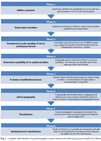
and See (2006), but it has been adapted to reflect the handling, processing and presentation of individual-level data (see Fig. 2). Note that the framework was developed using data from the 2001 census but any census data can be used provided there are accompanying microdata as outlined below.

Defining the Purpose

The overall purpose is to produce a generic, individual-level geodemographic classification that can be applied across a broad set of applications. For this reason a selection of variables from the 2001 UK census is used. To test the functionality of the classification, we have developed it for two contrasting areas: Leeds and Richmondshire, both in the Yorkshire region, UK. However, for this paper, we present only the results for the city of Leeds. Leeds was selected as it is close to the national average for a range of socio-economic variables (CASWEB2001; Leeds City Council2002).

Selecting the Input Data

All of the variables used to create the classification were obtained from the freely available Small Area Microdata (SAM) file in the UK census. SAM is an individual-level sample of anonymised records, which were extracted from the 2001 Census (ONS 2008). The SAM is similar to the SAR (Sample of Anonymised Records) with regards to variable inclusion, however, broader banding/categorising is adopted to preserve individual confidentiality given the personal nature of this multivariate dataset. The range of variables are also more restricted when compared to the national census dataset thus creating a trade-off between rich individual-level data and a diverse pool of variables to select from. Furthermore, the SAM provides a finer level of geography, i.e. the local authority (government) level, as opposed to the then larger government office regions (GORs) in the standard SAR, the latter discontinued in 2011. Local authorities are smaller, with population sizes ranging from ~1 million to 27,000 (Local Government Boundary Commission2014). The SAM sample accounts for 5% of the population and contains circa 2.9 million records from people in the UK and ~35,000 for the Leeds metropolitan district (of Leeds’715,402 2001 population) (Leeds = SAM code 67). A broad range of census topics are covered, including; employment, personal demographics and residential arrangements (ONS2008).

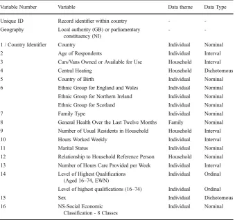
The data held in this file varies by type where each variable is categorised into one distinct category of (1) individual, (2) household, or (3) family. The file contains a total of seventy-four census variables, one unique identifier, plus thirteen ONS / Department of Food and Rural Affairs (DEFRA) variables and additional imputed variables. This research considers only the census variables. Examples of such variables include: number of cars / vans owned or available for use (household category), presence / number of dependent children in family (family category) and fundamental demo-graphic variables such as age / sex / ethnicity / social-economic classification of respondents (individual category). Table1contains the range of variables selected for inclusion in the classification together with the associated theme (individual, household or family) and data types.

Transforming and Re-scaling Variables

dissimilarity (Kaufman and Rousseeuw1990). To be able to do this effectively, the data first needs to be pre-processed to (i) convert the dichotomous and categorical-nominal variables to continuous data (ii) undertake any variable recoding and (iii) ensure polarity (data direction).

The variables in the SAM are of three kinds: dichotomous, categorical– nominal and categorical–ordinal, and do not lend themselves to typical clustering algorithms, which are generally used for segmenting continuous and/or ordinal variables only. The clustering algorithm used here is K-Means, which is an iterative relocation algorithm based upon an error sum of squares measure (Jain and Dubes1988), and also requires these data types. Thus, the first data pre-processing step was to convert the dichoto-mous and categorical-nominal variables to continuous data. Several adaptations to the algorithm have been proposed for handling mixed variable types (Ahmed and Day 2007; San et al.2004) but a different approach to aligning all variables was adopted here. The conversion was undertaken using variables that reflect income and/or wealth. With no such variables present in the census (excluding proxy measures), the British Household Panel Survey (BHPS) was selected (now part of Understanding Society, see: Understanding Society2015) instead. The‘Monthly Gross Income’variable [in Table 1 Selection of variables for SAM individual-level classification

Variable Number Variable Data theme Data Type

Unique ID Record identifier within country - -Geography Local authority (GB) or parliamentary

constituency (NI)

-

-1 / Country Identifier Country Individual Nominal

2 Age of Respondents Individual Interval

3 Cars/Vans Owned or Available for Use Household Interval

4 Central Heating Household Dichotomous

5 Country of Birth Individual Nominal

6 Ethnic Group for England and Wales Individual Nominal Ethnic Group for Northern Ireland Individual Nominal

Ethnic Group for Scotland Individual Nominal

7 Family Type Individual Nominal

8 General Health Over the Last Twelve Months Family Nominal 9 Number of Usual Residents in Household Household Interval

10 Hours Worked Weekly Individual Interval

11 Marital Status Individual Nominal

12 Relationship to Household Reference Person Household Nominal

13 Number of Hours Care Provided per Week Individual Interval

14 Level of Highest Qualifications (Aged 16–74, EWN)

Individual Ordinal

Level of highest qualifications (16–74) Individual Ordinal

15 Sex Individual Dichotomous

16 NS-Social Economic

Classification - 8 Classes

British Pound Sterling] (BHPS variable reference: RPAYG) was the most complete with regards to individual responses and therefore selected.

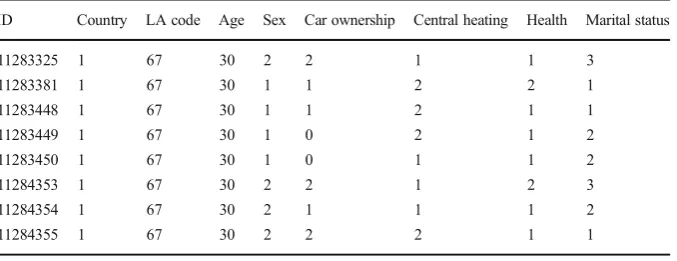
The equivalent SAM variable in the BHPS was extracted and the average gross monthly income for persons falling into each variable sub-category (e.g. marital status: single, widowed, divorced etc) was calculated. For this transformation to work, each of the variables selected for use in the classification had to be present in the BHPS. Table2 shows the original SAM data and Table3 shows the same data transformed into a monetary continuous scale for a small subset of the Leeds records. As examples, Central Heating: 1 = yes, 2 = no. Sex: 1 = male, 2 = female.

One should also note that the gross income figures listed above are averaged across the entire population (including those out of work, e.g. under 16’s, retired and unem-ployed) and are therefore lower than official average salary estimates noted elsewhere, such as in the Annual Survey of Hours and Earning (ONS2013). Without incorporating the entire population, the process would be misleading. However, for the purpose of effective clustering, it is the magnitude and level of difference between variables and variable sub-categories which is of most importance–more so than producing accurate salary estimates.

In order to achieve this process fully, re-coding of the data was necessary due to the structure / aggregation of the data between the SAM and BHPS. For example, some variables in the BHPS are continuous (e.g. age, hours worked per week, number of care hours provided) and therefore needed to be aggregated up to match the categories as put forward by the SAM. This was a simplistic summation process. However, other BHPS variables are also categorical and if the categorical variables in the BHPS failed to match the categorical variables in the SAM, e.g. BHPS contained a far greater number of groupings for Marital Status than the SAM, then some data matching was necessary. Using this example, the SAM assigns all individuals into one of three [legal] categories; Single (never married); Married, re-married; and Separated (but still legally married), Divorced or widowed. The BHPS separates individuals into nine groupings–including several extra categories not covered by the SAM, for example, Living as a couple; Have a dissolved civil partnership; Separated from a civil partnership; and Surviving partner of a civil partnership. Matching these individuals into the categories as put forward by the SAM required some decisions to be made prior to transformation to a continuous, monetary value. Figure 3 illustrates the process through which Marital

Table 2 Original SAM data prior to conversion to gross monthly income

ID Country LA code Age Sex Car ownership Central heating Health Marital status

11283325 1 67 30 2 2 1 1 3

11283381 1 67 30 1 1 2 2 1

11283448 1 67 30 1 1 2 1 1

11283449 1 67 30 1 0 2 1 2

11283450 1 67 30 1 0 1 1 2

11284353 1 67 30 2 2 1 2 3

11284354 1 67 30 2 1 1 1 2

Status within the BHPS was matched to that in the SAM. A similar matching process was also necessary for several other variables, including: Relationship to household reference person (HRP) (30 B.P. vs. 6 SAM categories) and NS-SEC (33 B.P. vs. 8 SAM categories).

Determining Suitability of Re-scaled Variables

A conversion to monetary values resulted in certain variables losing their desired meaning; age is the most noteworthy example. Once converted to a continuous scale, persons in the lower age groupings (0–4, 5–9, 10–15) were captured in ways identical to those in older categories and following retirement (generally 70+), as neither age group earns any form of salary (benefits and pensions excluded). For this reason, and given the impact this would have when clustering, variables deemed to be ordinal in their structure and of a format suitable for clustering in their original form were not transformed. These variables included: (1) Age, (2) Number of Hours Worked Per Table 3 Newly created gross monthly income values for SAM categories based on BHPS, in British Pound Sterling

ID Country LA code Age Sex Car ownership

Central heating

Health Marital status

11283325 1131.58 67 1702.20 1392.84 1077.38 1793.19 1826.79 1468.27

11283381 1131.58 67 1702.20 2225.09 923.26 1478.51 1626.93 1516.29 11283448 1131.58 67 1702.20 2225.09 923.26 1478.51 1826.79 1516.29

11283449 1131.58 67 1702.20 2225.09 549.68 1478.51 1826.79 2006.11

11283450 1131.58 67 1702.20 2225.09 549.68 1793.19 1826.79 2006.11 11284353 1131.58 67 1702.20 1392.84 1077.38 1793.19 1626.93 1468.27

11284354 1131.58 67 1702.20 1392.84 923.26 1793.19 1826.79 2006.11

11284355 1131.58 67 1702.20 1392.84 1077.38 1478.51 1826.79 1516.29

Week, (3) Number of Care Hours Provided, (4) Number of Residents in Household and (5) Number of Cars/Vans Available for Use. These variables are recorded as interval data in the SAM. By modifying these intervals to include only the first value within the interval, this ensured that the data were transformed to an ordinal format. For example, somebody residing in the 0–4 age group is recorded as having an age of 0 and somebody in the 5–9 age group is recorded as having an age of 5. With regards to the remaining variables, such as‘Hours Worked per Week’and‘Number of Care Hours Provided’, the top value in the range is utilised for classification. Therefore, in the example working 1–15 h per week, fifteen is put forward for clustering.

The National Socio-Economic Classification (NS-SEC, 8 Classes) variable also underwent some refinements. This variable was considered suitable for classifying under its original data structure (despite being nominal by definition) in the same way as the five variables stated above (e.g. 1 - Large employers & higher managerial occupations, 2 - Higher professional occupations, 3 - Lower managerial and profes-sional occupations, etc). This variable was left in its original form due to the fact that the final two categories where wholly incomplete resulting in zero average earnings per month. Although this variable is not designed to be hierarchical, it was decided to keep this in a continuous monetary format and estimate the two missing categories based on a combined average of the two nearest categories. Similar to the importance of gauging how (dis)similar individuals in the marital status category are, the same process was applied here.

Finally, the data were normalised and polarity was ensured, i.e. high values in all variables were positive and low values were negative (excluding any variables than may be regarded as neutral).

Classifying the Data

As referred to in Transforming and Re-scaling Variables section, K-Means was employed as the clustering algorithm. The algorithm functions iteratively, moving a case from one cluster to another to see if the move would enhance the sum of squared deviations within each cluster (Aldenderfer and Blashfield1984). The case will then be allocated (or re-allocated) to the cluster to which it brings the maximum improvement. The next iteration takes place when all the cases have been processed. A stable classification is therefore achieved when no moves occur during a full iteration of the data. After clustering is complete, it is then possible to inspect the means of each cluster (i.e. the cluster centres) to gauge the distinctiveness of the clusters (Everitt et al.2011). K-Means was applied to the data and the number of clusters was experimented with based on suggestions made by Milligan (1996) and Gibson and See (2006) whereby a process of classification iteration took place to deduce the change in the slope of the scree. A classification with five clusters was chosen to evidence the functionality of the framework. This decision was largely down to the data loss that is generally experi-enced when extending beyond a higher number of groupings, something illustrated by the percentage of Within cluster Sums of Squares (%WSS), and to ensure ease of comparability between districts.

UK-wide classification or to contrast two areas in different constituent countries of the UK (England, Wales, Scotland or Northern Island) then such a variable is worthy of use – hence its inclusion as part of the wider framework. The resulting classification is therefore based on the remaining fifteen individual-level variables from Table1.

Adding the Geographical Component

The final phase in constructing the classification involved the addition of geography. It is important to emphasise the value of geography in order to avoid producing a purely sociological classification of individuals and ensure any neighbourhood effects present in traditional areal systems are captured.

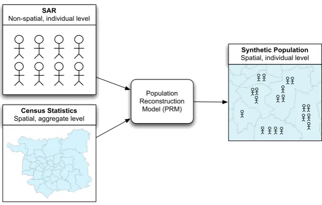
The classification was linked to an individual population for Leeds that was generated using spatial microsimulation. Microsimulation creates a synthetic popula-tion drawn from an anonymous sample of individual-level data, that ‘realistically’ matches the observed population (see Fig.4for an illustration). Spatial microsimulation allows neighbourhood effects to be captured.

The process follows the steps detailed below:

1 A population of individuals, termed the sample, is obtained (normally from the UK Census). This sample represents a higher spatial level, such as a country or one of its statistical areas.

2 To create a population for a smaller geographical area (such as Leeds’output areas used in this study) weights are applied to each member of the sample. For example, if the small area is multi-ethnic, we may wish to apply high weights to members of the sample whose country of birth is outside the UK.

3 For each small area, a series of constraint tables that count the distribution of characteristics in the population for a range of attributes are used.

The overall objective of the microsimulation is to generate a set of weights so that when the sample population is aggregated, the goodness of fit between the model distributions and the equivalent constraints is maximised. There are several algorithms that can be used to achieve this, including deterministic reweighting (Ballas et al. 2005), conditional probabilities (Birkin and Clarke1988) and combinatorial optimisa-tion (Voas and Williamson2000). Following the recommendation of Harland et al. (2012), the combinatorial optimisation approach was used. This algorithm uses the simulated annealing approach to optimise the number of matches in the synthetic population. The synthetic population was generated using the Flexible Modelling Framework (Harland2013).

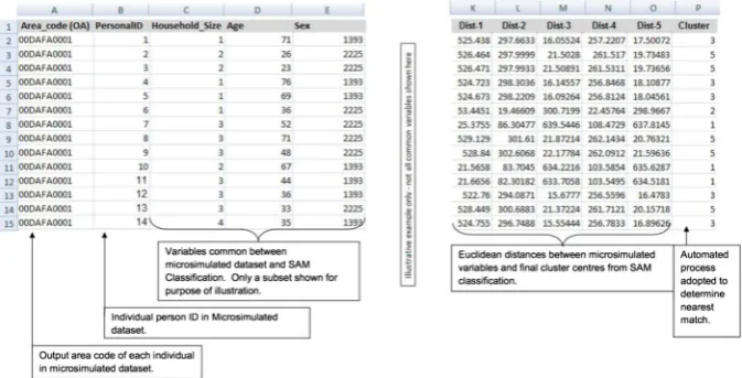
The 715,402 individuals (2001) were synthesised at output area level (2438 areas) using constraint data acquired from the Census of Population via CASWEB (2001) and survey data courtesy of the British Household Panel Survey. These synthetic individ-uals, which are geographically referenced via output area, were then linked to the SAM-based classification using common variables in order to assign a cluster code from the classification to each individual.

The purpose of this link is to attribute each member of the complete population a cluster code based on the classification generated on the modified SAM data. This then ensures all members of the population have a cluster code (indicative of their behaviour) and an output area reference enabling the capture of the aforementioned notion of neighboured. Should this be based purely on the SAM data, any analysis would be restricted to the local authority level and hence the influence of neighbourhood would be lost.

The eight variables common between the classification and microsimulated dataset were first converted into SAM-identical format (i.e. monetary income values or ordinal equivalents). Then, the Euclidean distance between each individ-ual and the SAM cluster centres were calculated (the final distance was divided by 10,000 in all cases to reduce the magnitude of the values and allow for ease of interpretation). The cluster with the minimum distance was then assigned to each microsimulated individual. Figure 5 illustrates this process. Although the chosen

method adopts crisp clustering, it does provide a fuzzy-like representation of individuals in each output area, thereby reducing the ecological fallacy associated with a purely area-based crisp geodemographic classification.

Visualising and Understanding the Output

Given the supplementing with geography process undertaken in phase 6, visualisation was carried out based on the modal cluster membership of each individual per Leeds output area. Although this involved the aggregation of individual-level data and hence a move back towards area-based geodemographics, it was executed here entirely for the purpose of understanding the predominant geographical distribution of individuals.

Validation and Enrichment

This final phase represents an opportunity to both validate and enrich the results with supplementary information. The ability to link the final individual-based classification to external non-census datasets provides a means of profiling far deeper against more behavioural and lifestyle information. Not only does this add value to a classification through enrichment, but it can also be used for validation purposes. For example, one might expect any cluster categorised as being predominantly young, city-living types to being technologically advanced or physically active. Given that a system built entirely on census data cannot benchmark against such variables, the ability to link the classification to survey datasets like the BHPS, which contains variables of this nature, adds real value. It also gives users of these external datasets an alternative method through which to view their data.

Through a process of statistical matching (identical to phase 6), the cluster codes from the classification were appended onto other datasets. It was possible to match the cluster codes onto the BHPS dataset and profile the results against other variables (principally behavioural) such as an individual’s propensity to dine out of an evening or take flights abroad during the course of a twelve-month period. Such outcomes not only add value and enrich the classification but also offer an opportunity to corroborate the clustering process.

Results

This section shows the results of the individual-based classification, i.e. phases 7 and 8 of the framework (Fig.2), for Leeds.

Results from Phase 7: Analysis of Clusters

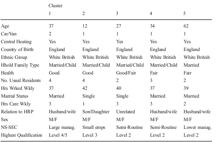
Cluster centres are an important way of analysing cluster composition. The results from the final cluster centres provide broad indications as to the typical population charac-teristics within each cluster and are listed in Table4for Leeds. Table5 interprets the output from Table4and illustrates this in a more understandable format.

Table 4 Final cluster centres for Leeds SAM classification

Cluster

1 2 3 4 5

Age 37 12 27 34 62

Car/Van 2 1 1 1 1

Central Heating 1763.04 1734.71 1710.29 1688.30 1727.87

Country of Birth 1501.15 1501.15 1501.15 1501.15 1501.15 Ethnic Group 1240.7823 1321.7341 1332.7169 1292.8687 1324.4129

Hhold Family Type 1728.85 1732.57 1726.25 1777.04 1856.35

Health 1779.41 1798.71 1763.25 1753.40 1735.88

No. Usual Residents 4 4 2 3 2

Hrs Wrked Wkly 37 42 40 37 39

Marital Status 1789.32 1535.78 1750.31 1978.24 1773.27

Hrs Care Wkly 3 1 3 3 2

Relation to HRP 1597.48 241.13 446.55 1586.08 1664.01

Sex 1785.56 1784.42 1788.36 1781.15 1780.24

NS-SEC 2170.17 1708.64 867.35 732.26 1587.72

Highest Qualification 2491.07 1566.84 1304.71 1323.25 1344.75

Table 5 Interpreted cluster centres for Leeds SAM classification

Cluster

1 2 3 4 5

Age 37 12 27 34 62

Car/Van 2 1 1 1 1

Central Heating Yes Yes Yes Yes Yes

Country of Birth England England England England England

Ethnic Group White British White British White British White British White British Hhold Family Type Married/Child Married/Child Married/Child Married/Child Married

Health Good Good Good/Fair Fair Fair

No. Usual Residents 4 4 2 3 2

Hrs Wrked Wkly 37 42 40 37 39

Marital Status Married Single Single Married Married

Hrs Care Wkly 3 1 3 3 2

Relation to HRP Husband/wife Son/Daughter Unrelated Husband/wife Husband/wife

Sex M/F M/F M/F M/F M/F

naming conventions in a way similar to that adopted in conventional area-based geodemographics. The profiles for Leeds are detailed below:

Cluster 1: Affluent Managers

This cluster is a middle-aged cluster with an average age of thirty-seven years. Typically households are quite affluent as reflected by access to two cars, being largely employed in managerial capacities. Members of this cluster provide some weekly care for relatives and work typical hours. Members tend to be married and live in house-holds with circa four people, likely to include children. Individuals in this cluster are typically of White British ethnicity and well educated.

Cluster 2: Young People living with Family

This cluster contains a youthful and healthy demographic with an average age of twelve years. These individuals live with their parents who are married, have good general health and are of White British ethnicity. The household has access to one car, is heated and on average houses around four people. They are the son/daughter of the head of household.

Cluster 3: Co-habiting Couples

This cluster is categorised by young individuals with start-up families. Members of this cluster tend to be single by legal definition but may be cohabiting. Individuals are in their mid/late twenties, have access to a car and work predominantly in semi-routine occupations with employment taking up to circa forty hours per week. Members have some education and are typically in good to fair health.

Cluster 4: Average Resident

This cluster is categorised by individuals in their mid-thirties who are married with children. Health is recorded as fair and members have some education, and work typical length weeks. Households typically contain three individuals with care provided for family on a weekly basis. Education levels are fair and access to a car is common.

Cluster 5: Nearing Retirement

This cluster contains an elderly demographic with a typical age of sixty-two. Members tend to be married without children at home and in fair health. Of those still working, most work in lower managerial occupations and have some education. The average sized household is two persons with most married and of a White British Ethnicity.

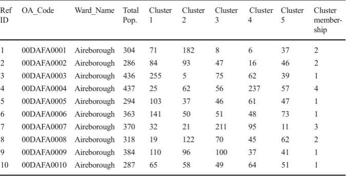
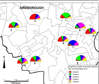
A sample of ten output areas are shown in Table6to provide an overview of how the cluster allocation process was carried out.

Cluster 1, categorised by individuals in higher managerial occupations and in 2+ car households, tends to be distributed in the more affluent areas of the city, in particular to the north and with some presence in the east. To the contrary, Clusters 3 and 4, which may be regarded as the less affluent cluster-types given the semi-routine occupations (probably leading to longer working weeks as also identified in the classification), fair health and, in the case of cluster 3, persons sharing houses who are unrelated, show different patterns. These clusters are focused more around the inner city (in the case of cluster 4) and to a lesser extent cluster 3, the latter also being more sporadic it its spatial patterns. Cluster 5, typified by elderly populations, arguably does not follow the conventional spatial patterns one would expect in a UK city; however, it is principally occupied by people in menial employment, which may hinder mobility.

Figure6presents an alternative way of visualising the true demographic composi-tion of an area. The proporcomposi-tion of each cluster is highlighted within a given output area, which introduces a level of fuzziness to the presentation. The ten output areas listed in Table 6 are shown in Fig. 6 which demonstrates the variability of individual types across space but can also be used as a tool for the exploration of patterns.

Results from Phase 8: Validating and Adding Value

Through adopting a process akin to the statistical matching method discussed when linking the SAM cluster codes to the simulated datasets and small-area geography, it is possible to link the classification cluster codes to external datasets. The only require-ment is the presence of common variables between the two datasets to enable the codes to be matched. To illustrate this process, a link to the BHPS (wave 18) was established. This link enabled each of the individual records in the BHPS to be assigned to one of five SAM clusters.

Variables present in the BHPS are designed to describe socio-economic conditions at both individual and household level (ISER2011). Variable categories include; house-hold organisation, employment, accommodation, tenancy, income and wealth, housing, Table 6 First ten Leeds output areas (sorted A-Z) and associated cluster codes

Ref ID

OA_Code Ward_Name Total Pop.

Cluster 1

Cluster 2

Cluster 3

Cluster 4

Cluster 5

Cluster member-ship

1 00DAFA0001 Aireborough 304 71 182 8 6 37 2

2 00DAFA0002 Aireborough 286 84 93 47 16 46 2

3 00DAFA0003 Aireborough 436 255 5 75 62 39 1

4 00DAFA0004 Aireborough 437 25 62 56 237 57 4

5 00DAFA0005 Aireborough 294 103 37 46 61 47 1

6 00DAFA0006 Aireborough 363 141 50 51 48 73 1 7 00DAFA0007 Aireborough 370 32 21 211 95 11 3

8 00DAFA0008 Aireborough 318 19 122 70 45 62 2

health, socio-economic values, residential mobility, marital and relationship history, social support, and individual and household demographics (ISER2011) and hence add value over and above the variables present in the original SAM file. Furthermore, the extensive choice of variables within the BHPS made it easy to ensure a robust link between this data file and the SAM classification. Of the fifteen variables used to create the SAM classification, fourteen were present in the BHPS. The results are shown in Table7.

As can be seen from Table7, if taking the full cluster descriptors into consideration, the results appear to corroborate the cluster characteristics to some degree. However, there are a series of anomalies that may be explained by the methods adopted.

than decisions made by the individuals specifically assigned to this cluster. Hence this links back to more coarse spatial units influencing the individual (household, neighbourhood, environment etc).

A second example can be seen from assessing Cluster 1 (Affluent Managers). As many of the variables presented in Table7can be linked to availability of disposable income, it is unsurprising that members of this cluster have a high tendency to dine out once per month (greater than other clusters) and attend sporting venues. The high proportion of members willing to vote (the only cluster where‘No Vote’is not highly ranked) in addition to an alignment towards the Conservative Party are also statistics that corroborate the cluster output. The low percentage partaking in sport is rather surprising. A key observation to be highlighted is the use of Leeds’final cluster centres when classifying the complete BHPS (wave 18). Naturally, different parts of the UK look rather different in terms of their demographic profiles and the use of Leeds’cluster centres may have impacted on the results of this BHPS linkage process–particularly given that the BHPS is UK-wide. Furthermore, adopting the complete BHPS file as Table 7 Contrasting SAM Classification with BHPS Individuals and extracting new information

Cluster Dine out? Play sport? Political

allegiance (if voting tomorrow)?

Watch live sport (at sporting venue)?

1. Affluent Managers Once Per Month–60%

Once per week–3%

No vote–50% Several Times per Year–20% Conservative–25%

Other Party–8.3% Several Times per

Year–22%

Labour–8% Liberal Democrat–8% 2. Young People living

with Family

Once Per Month–35%

Once per week–7%

No vote–40% Several Times per Year–8% Can_’t Vote_–18.6%

Several Times per Year–40%

Labour_–12% Conservative–9.3% Liberal

Democrat–5.8% 3. Co-habiting Couples Once Per

Month–47%

Once per week–6%

No vote–50.4% Several Times per Year–14% Conservative–12.2%

Several Times per

Year–30% Labour–8.5% Liberal Democrat_–6% 4. Average Resident Once Per

Month–44%

Once per week–6%

No vote–48.2% Several Times per Year–14% Conservative–11.7%

Several Times per

Year–31% Labour–10% Can’t Vote–8% Liberal

Democrat–6.2% 5. Nearing Retirement Once Per

Month–36%

Once per week–8%

No vote–47.5% Several Times per Year–9% Conservative–12.5%

Several Times per Year–31%

opposed to a more regionalised subset may also have had some bearing on the results presented in Table7.

Discussion and Conclusions

The framework presented and discussed in this paper is one of the first fully open and transparent methodologies geared towards individual-level classification that uses only data from the UK census. It achieves the goal of producing a geodemographic classification at the person unit. Inevitably, however, the framework is not the finished product nor is it without its problems but it does provide reason to maintain the pursuit of individual-level classification as the ultimate in geodemographic analysis. Although it was demonstrated using data from the 2001 census, it can be applied to any census where there are small area microdata.

The proposed framework combines added discrimination with reduced ecological fallacy impact through operating at the level of the individual. If a system is deemed to discriminate better than alternatives, then it will, as a consequence, reduce the level of ecological fallacy as the clusters are likely to be more homogeneous. As highlighted previously, as the quantity of variables increases in an aggregate-data classification, the scope for misrepresentation also increases as fewer people are likely to fit the described cluster demographic. At the level of the person, although this is also the case, it is easier to maintain a greater level of homogeneity as one individual can easily be re-classified should he/she not fit a given cluster definition. It is only through supplementing with geography that the issue of ecological fallacy really arises.

In terms of weaknesses, within this framework certain variables do not appear to differentiate between individuals particularly well. Such variables include ethnic group and gender. Even though these variables may be termed fundamental census charac-teristics, later versions of this framework may be required to make more detailed decisions on the variables included. Furthermore, a means of handling high valued continuous monetary variables and low valued ordinal variables is important should this framework successfully evolve. Nonetheless, this research acts as the first piece of academic work to attempt to classify individual person-level data in this way and incorporate small-area geography and linkages to external datasets for both validation and deeper profiling.

The inter-disciplinary opportunities that profiling at this level generates, in particular with an ability to profile against external datasets, offers a broad appeal to further research using this framework. This work has demonstrated an ability to link to the BHPS and explore behavioural datasets over and above pure census characteristics held directly within the classification. Opportunities therefore exist to profile against datasets such as the Health Survey for England, the Crime Survey for England and Wales and the National Travel Survey. When one considers the refinement of the framework in addition to such diverse profiling opportunities, scope for research extension is clear and policy implications brought about from more accurate and finer-level classifica-tions offer incentives to pursue this research direction.

Open AccessThis article is distributed under the terms of the Creative Commons Attribution 4.0 International License (http://creativecommons.org/licenses/by/4.0/), which permits unrestricted use, distribution, and repro-duction in any medium, provided you give appropriate credit to the original author(s) and the source, provide a link to the Creative Commons license, and indicate if changes were made.

References

Abbas, J., Ojo, A., & Orange, S. (2009). Geodemographics: A tool for health intelligence?Public Health, 123, 35–39.

Acxiom (2016). Welcome to PersonicX, Available at:http://www.personicx.co.uk/personicx.html. Accessed 31 July 2017.

Adnan, M., Longley, P., Singleton, A., & Brunsdon, C. (2010). Towards real-time geodemographics: Clustering algorithm performance for large multidimensional spatial databases. Transactions in GIS, 14(3), 283–297.

Ahmed, A., & Day, L. (2007). A K-mean clustering algorithm for mixed numeric and categorical data.Data & Knowledge Engineering, 63, 503–527.

Aldenderfer, M., & Blashfield, R. (1984).Cluster analysis. Beverly Hills: Sage Press.

Ashby, D. I., & Longley, P. A. (2005). Geocomputation, Geodemographics and resource allocation for local policing.Transactions in GIS, 9, 53–72.

Ballas, D., Clarke, G., Dorling, D., Eyre, H., Thomas, B., & Rossiter, D. (2005). SimBritain: A spatial microsimulation approach to population dynamics.Population, Space and Place, 11, 13–34.

Birkin, M. (1995). Customer targeting, Geodemographics and lifestyle approaches. In P. Longley & G. Clarke (Eds.),GIS for business and service planning. Cambridge, GeoInformation.

Birkin, M., & Clarke, M. (1988). SYNTHESIS - a synthetic spatial information system for urban and regional analysis: Methods and examples.Environment and Planning A, 20, 1645–1671.

Burns L. (2017). Creating a health/deprivation geodemographic classification system using K-means cluster-ing methods. Available online at: http://methods.sagepub.com/case/health-deprivation-geodemographic-classification-system-k-means-clustering. Accessed 2 Aug 2017.

Cadman, E. (2014). UK census to go ahead in 2021. Available online at:https://www.ft.com/content/4313 fd34-1586-11e4-9e18-00144feabdc0. Accessed 3 Aug 2017.

CASWEB (2001).(Now: UK data service),http://casweb.mimas.ac.uk/. Accessed: 3 Oct 2015.

Crooks, A., Heppenstall, A., & Malleson, N. (2018). Agent-based modelling. In B. Huang (Ed.), Comprehensive Geographic Information Systems. Amsterdam: Elsevier.

Everitt, B., Landau, S., Leese, M., & Stahl, D. (2011).Cluster analysis(5th ed.). London: Arnold. Experian (2015). Mosaic USA: The consumer classification solution for consistent cross-channel marketing.

Available online at:https://www.experian.com/assets/marketing-services/brochures/mosaic-brochure.pdf. Accessed 6 Aug 2017.

Farr, M., & Webber, R. (2001). MOSAIC: From an area classification system to individual classification. Journal of Targeting, Measurement and Analysis for Marketing, 10(1), 55–65.

Gibson, P., & See, L. (2006). Using Geodemographics and GIS for sustainable development. In M. Campagna (Ed.),GIS for sustainable development. London: Taylor and Francis.

Harland, K. (2013).Microsimulation model user guide (flexible modelling framework). NCRM: NCRM Working Paper.

Harland, K., Heppenstall, A., Smith, D., & Birkin, M. (2012). Creating realistic synthetic populations at varying spatial scales: A comparative critique of population Synthesis techniques.Journal of Artificial Societies and Social Simulation, 15(1), 1–15.

Harris, R., Sleight, R., & Webber, R. (2005).Geodemographics, gis and neighbourhood targeting. Chichester: Wiley.

Institute for Social and Economic Research (ISER) (2011). British household panel survey,https://www.iser. essex.ac.uk/bhps. Accessed 1 Oct 2015.

Jain, A., & Dubes, R. (1988).Algorithms for clustering data. Englewood Cliffs: Prentice Hall. Kaufman, L., & Rousseeuw, P. J. (1990).Finding groups in data. New York: Wiley.

Leeds City Council (2002),2001 Census - First Results for Leeds, available online at:http://www.leeds.gov. uk/docs/2001%20Census%20key%20points.pdf, [Accessed: 13/10/2015].

Local Government Boundary Commission (2014),Local Authorities in England, available online at:

https://www.lgbce.org.uk/records-and-resources/local-authorities-in-england, [Accessed: 15/10/2015]. Longley, P. (2017), Geodemographic profiling inThe International Encyclopaedia of Geography, John Wiley

Milligan, G. (1996). Clustering validation: Results and implications for applied analyses. In P. Arabie, L. J. Hubert, & G. De Soete (Eds.),Clustering and classification. Singapore: World Scientific.

Office for National Statistics [ONS] (2008),Samples of Anonymised Records, available online at:http://www. ons.gov.uk/ons/guide-method/census/census-2001/data-and-products/data-and-product-catalogue/microdata/samples-of-anonymised-records/samples-of-anonymised-records.html, [Accessed: 12/10/2015].

Office for National Statistics [ONS] (2012),Census Geography, Available online at:https://www.ons.gov. uk/methodology/geography/ukgeographies/censusgeography, [Accessed: 02/08/2017].

Office for National Statistics [ONS] (2013),Annual Earnings, available online at:http://www.ons.gov. uk/ons/taxonomy/index.html?nscl=Annual+Earnings, [Accessed: 15/10/2015].

Office for National Statistics [ONS] (2014),Postal Geography, Available online at:http://www.ons.gov. uk/ons/guide-method/geography/beginner-s-guide/postal/index.html, [Accessed: 13/10/2015].

Openshaw, S. & Wymer, C. (1995), Classification and regionalization, census Users'handbook,inOpenshaw, S. (Ed.), GeoInformation International, Cambridge p.239–270.

Petersen, J., Gibin, M., Longley, P., Mateos, P., Atkinson, P., & Ashby, D. (2011). Geodemographics as a tool for targeting neighbourhoods in public health campaigns.Journal of Geographical Systems, 13(2), 173–192. San, O., Huynh, V., & Nakamori, Y. (2004). An alternative extension of the k-means algorithm for clustering

categorical data.International Journal of Applied Mathematics and Computer Science, 14(2), 241–247. Singleton, A. D., & Longley, P. A. (2009). Creating open source geodemographics: Refining a national classification of census output areas for applications in higher education.Papers in Regional Science, 88, 643–666.

Singleton, A., & Spielman, S. (2014). The past, present, and future of geodemographic research in the United Kingdom.The Professional Geographer, 66(4), 558–567.

Understanding Society (2015),BHPS–A guide to how it is used in Understanding Society. Available online at:https://www.understandingsociety.ac.uk/about/bhps-in-understanding-society, [Accessed: 03/08/2017]. Vickers, D. & Rees, P. (2006), Introducing the area classification of output areas,Population Trends, pp. 15– 29. Available online at:https://www.ons.gov.uk/ons/rel/population-trends-rd/population-trends/no–125–

autumn-2006/population-trends-pt2.pdf, [Accessed: 31/07/2017].

Vickers, D., & Rees, P. (2007). Creating the UK National Statistics 2001 output area classification.Journal of the Royal Statistical Society: Series A, 170(2), 379–403.