White Rose Research Online URL for this paper:
http://eprints.whiterose.ac.uk/129134/
Version: Accepted Version
Article:
Chen, Lejun, Pomfret, Andrew James orcid.org/0000-0003-0325-1617 and Clarke, Timothy
orcid.org/0000-0002-5238-4769 (2018) Multistage Output-lifting Eigenstructure
Assignment: A Multirate Ball and Plate Example. International Journal of Control. pp. 1-32.
ISSN 0020-7179
https://doi.org/10.1080/00207179.2018.1459856
Reuse
Items deposited in White Rose Research Online are protected by copyright, with all rights reserved unless indicated otherwise. They may be downloaded and/or printed for private study, or other acts as permitted by national copyright laws. The publisher or other rights holders may allow further reproduction and re-use of the full text version. This is indicated by the licence information on the White Rose Research Online record for the item.
Takedown
If you consider content in White Rose Research Online to be in breach of UK law, please notify us by
For Peer Review
! "
For Peer Review
Vol. 00, No. 00, Month 20XX, 1–24
Multistage Output-lifting Eigenstructure Assignment: A Multirate Ball and Plate Example
(Received 00 Month 20XX; accepted 00 Month 20XX)
By exploiting both the left and the right allowable subspaces in consecutive stages, this paper extends a recently-developed output-lifting eigenstructure assignment approach into a multistage eigenstructure assignment scheme. In this scheme, design degrees of freedom, enlarged via output-lifting, are further exploited to improve eigenvector assignment. To mitigate the inherent conflicts between the theoretical development of eigenstructure assignment and inherent physical system characteristics, the paper also clearly demonstrates how to derive an ideal eigenstructure, particularly the desired eigenvectors, to distribute and decouple the natural modes among appropriate states or outputs, based upon an example: a novel multirate Ball and Plate system. The design and simulation results show the efficacy of the scheme.
Keywords:lifting; eigenstructure assignment; ball and plate system; allowable subspace
For Peer Review
Nomenclature
The reader is referred to Figures 1 to 3.
a Length of the plate
b Width of the plate
˜b Damping constant of the rotational mechanical system
d Ball displacement relative to the plate
fx External force applied at x
fy External force applied on y
h Ball vertical displacement along ok Ii Armature current flow into theith motor
Jb Moment of Inertial of the ball
Jm Moment of inertia of the rotor
Jp Moment of Inertial of the plate
Ke Motor constant related to the back electromotive force
Kt Electromotive force constant
l Length of the motor shaft
La Armature induction
m Mass of the ball
mωx Moment applied to the ball along ωx
mωy Moment applied to the ball alongωy ˜
p Plate angular velocity alongoi
˜
q Plate angular velocity alongoj
˜
r Plate angular velocity alongok
rb Radius of the ball
Rm Armature resistance
s Ball displacement relative to the earth ¯
s1 Ball displacement along oi
¯
s2 Ball displacement along oj
Vi Input voltage applied to the armature of the ith motor
x Ball displacement alongol y Ball displacement along om Zi Vertical displacements of three push-rods
αi Rotation angle of three DC motor
φ Plate rotation angle alongol θ Plate rotation angle alongom ω Ball angular velocity relative to the earth
ωp Plate angular velocity relative to the earth
ωx Ball angular velocity alongol
ωy Ball angular velocity along om
ωz Ball angular velocity along on
1. Introduction
Through synthesizing a feedback gain matrix that matches the closed-loop eigenstructure as closely as possible to an ideal set, eigenstructure assignment (EA) ensures some useful properties such as stability robustness, desired transient response, mode decoupling and disturbance rejection (Alireza & Batool, 2012; B. Chen & Nagarajaiah, 2007; Duval, Clerc, & LeGorrec, 2006; Farineau, 1989; Kshatriya, Annakkage, Hughes, & Gole, 2007; Lhachemi, Saussie, & Zhu, 2017; G. P. Liu &
For Peer Review
ton, 1998; Y. Liu, Tan, Wang, & Wang, 2013; Moore, 1976; Ntogramatzidis, Nguyen, & Schmid, 2015; Ouyang, Richiedei, Trevisani, & Zanardo, 2012; Patton, Liu, & Patel, 1995; Piou & Sobel, 1994, 1995; Pomfret & Clarke, 2009; Wahrburg & Adamy, 2013; White, 1995; White, Bruyere, & Tsourdos, 2007). Compared with many competitive approaches that only achieve placement of the desired eigenvalues of the closed-loop system, EA additionally manipulates the direction of the eigenvectors. These define how system inputs will affect system modes and how system modes will be assigned to system states/outputs. Thus realistic control effect or the quality of control perfor-mance, e.g. the handling qualities of a flight controlled aircraft, can be achieved in a straightforward manner. Furthermore, EA ensures a ‘visible’ design process which may reduce time consumed in post-processing for tuning purposes. The development of EA has not been widely persued in the recent years due to a) traditional EA, particularly output feedback EA, requiring significant design degrees of freedom (DoF) (Andry, Shapiro, & Chung, 1983; Clarke, Ensor, & Griffin, 2003; Clarke & Griffin, 2004; Clarke, Griffin, & Ensor, 2003; Pomfret, Clarke, & Ensor, 2005; Roppenecker & O’Reilly, 1989; Srinathkumar, 1978; Zhao & Lam, 2016a, 2016b). b) Very few works (Clarke, En-sor, & Griffin, 2003; Garrard, Low, & Prouty, 1989; Low & Garrard, 1993) attempting to analyze how to derive an ideal eigenstructure, particularly the ideal eigenvectors, that reflect the inherent physical characteristics of the target system. This paper aims to cope with above two bottlenecks. In the literature, Piou and Sobel (1994, 1995) developed the multirate EA approach, but the concept of ‘lifting’ (T. Chen & Francis, 1995) was not taken into account. The lifting framework and EA were first time combined by Patton et al. (1995) to enlarge DoF, however this approach only lifted system inputs and generated inter-sample ripple. Recently, L. Chen, Pomfret, and Clarke (2017) developed output lifting EA which largely improved DoF and the single-rate full state feedback eigenstructure can be assigned in an output feedback framework, particularly when the Kimura condition (Kimura, 1975) is not satisfied.
Although output-lifting allows full state feedback eigenstructure to be assigned from the right allowable subspace, an exact assignment of desired eigenvectors (i.e. assignment of exactly the same elements of each eigenvector) is difficult to be achieved due to the limited dimension of the allowable right subspace determined by the number of system inputs. Since output-lifting only enlarges the effective number of system outputs, the dimension of the right allowable subspace is invariant. If only the right allowable subspace is used for eigenvector assignment, the maximum number of exactly assignable elements of each eigenvector, which equates to the number of system inputs, cannot be enlarged anymore. Exploiting the fact that output-lifting has the capability to enlarge the number of effective system outputs, the dimension of the left allowable subspace is thus increased. If the dimension of the left allowable subspace becomes larger than one of the right allowable subspace after output-lifting, a left allowable subspace based eigenvector assignment can further improve achieved eigenvectors and allows more elements of each eigenvector to be exactly assigned. Instead of only using the right allowable subspace for eigenvector assignment (the maximum number of exactly assignable elements of each eigenvector equates to the number of system inputs), this paper developed a multistage output-lifting EA scheme in which both the left and right allowable subspaces are used for EA. In the second stage where the left allowable subspace is used for eigenvector assignment, the partially assigned eigenvectors should contain more elements of desired eigenvectors due to output-lifting.
To mitigate the inherent conflict between the theoretical development of EA with the actual
system inherent physical characteristics, this paper also clearly demonstrates how to derive an ideal eigenstructure based upon a genuine example of a novel mutirate Ball and Plate system. Not only are the natural modes of Ball and Plate system decoupled and distributed in appropriate states or outputs, but also the eigenvectors are derived to be consistent with the physical relationships between Ball and Plate system states. Due to an otherwise lack of DoF, multistage output-lifting EA is applied to Ball and Plate system.
For Peer Review
left allowable subspace. b) demonstration of how to determine a practical eigenstructure using a Ball and Plate system example. Compared with other methods described in the literature (Garrard et al. (1989); Low and Garrard (1993)), a more transparent approach to selecting a set of ideal eigenvectors, parameterised by the desired eigenvalues, is developed in this paper.
The remainder of the paper is outlined as follows: Section 2 briefly introduces output-lifting EA, followed by the development of multistage output-lifting EA in Section 3. The mathematical model of a Ball and Plate system is developed in Section 4. Section 5 describes how the derive an ideal eigenstructure based upon the system physical characteristics. In Section 6, multistage output-lifting EA is then applied to this Ball and Plate system. The design and simulation results demonstrate the efficacy of the scheme.
2. Output-lifting eigenstructure assignment
In this section, the output-lifting EA approach (L. Chen et al., 2017) will be introduced briefly. Consider a discrete-time, controllable and observable linear time-invariant system
˙
x=Ax+Bu
y=Cx+Du (1)
where A ∈ Rn×n, B ∈ Rn×r, C ∈ Rm×n and D ∈ Rm×r are matrices with rank(B) = r and
rank(C) =m. Suppose the system in (1) is discretized at the base sampling periodTb which is any common factor of the input and output sampling periods. Furthermore, the hold circuit and the sampler work with sample periods ofqiTb andpoTb respectively. Then the main sampling period of the system becomesT = l.c.m(po, qi)∗Tb where l.c.m stands for least common multiple. Suppose system inputs and outputs are lifted byq andp respectively, where
q= l.c.m(po, qi)
qi
and p= l.c.m(po, qi)
pi
(2)
denote the input ratio and the output ratio, respectively. As in T. Chen and Francis (1995), a controllable and observable lifted system has the form
x(k+ 1) =ALx(k) +BLu¯(k) ¯
y(k) =CLx(k) +DLu¯(k)
(3)
wherex(k) :=x(kT). In (3), lifted inputs ¯u(k) and outputs ¯y(k) are
¯
u(k) :=
⎡
⎢ ⎢ ⎢ ⎢ ⎢ ⎣
u(kT)
u(kT+pTb)
u(kT+ 2pTb) .. .
u(kT + (pq−p)Tb)
⎤
⎥ ⎥ ⎥ ⎥ ⎥ ⎦
¯
y(k) :=
⎡
⎢ ⎢ ⎢ ⎢ ⎢ ⎣
y(kT)
y(kT +qTb)
y(kT + 2qTb) .. .
y(kT+ (pq−q)Tb)
⎤
⎥ ⎥ ⎥ ⎥ ⎥ ⎦
(4)
For Peer Review
and the matricesAL∈Rn×n, BL∈Rn×qr, CL∈Rpm×n and DL∈Rpm×qr are
AL BL
CL DL :=
⎡
⎢ ⎢ ⎢ ⎢ ⎢ ⎢ ⎢ ⎢ ⎢ ⎣
Apq pq−1
i=pq−p
AiB pq−p−1
i=pq−2p
AiB · · · p−1
i=0
AiB
C D0,0 D0,1 · · · D0,q−1
CAq D
1,0 D1,1 · · · D1,q−1
CA2q D
2,0 D2,1 · · · D2,q−1
..
. ... ... . .. ...
CApq−q D
p−1,0 Dp−1,1 · · · Dp−1,q−1
⎤
⎥ ⎥ ⎥ ⎥ ⎥ ⎥ ⎥ ⎥ ⎥ ⎦
(5)
where the element Di,j is defined as
Di,j =DX[jp,(j+1)p)(iq) +
(j+1)p−1
h=jp
CAin−1−hBX[0,iq)(h) (6)
and the characteristic function on integers X[a,b)(h) is
X[a,b)(h) =
I a≤h < b
0 otherwise
From (5), the number of effective system inputs and outputs are enlarged (i.e.r→qrandm→pm) and therefore extra DoF may be parameterised for the synthesis of the gain matrixK ∈Rr×pm. In this paper, the eigenvalues are assumed to be self-conjugate and pole-assignable. This assumption ensures the gain matrixK is real (Kimura, 1977). Applying an static output feedback law ¯u(k) =
Ky¯(k) + ¯r(k) to (3) yields the closed-loop system
x(k+ 1) = (AL+BLN CL)x(k) + (BL+BLN DL)¯r(k) ¯
y(k) = (CL+DLN CL)x(k) + (DL+DLN DL)¯r(k)
(7)
where ¯r represents lifted exogenous inputs and
N = (I−KDL)−1K (8)
Using the fact that theith distinct closed-loop right eigenpair (a pair of eigenvalue and eigenvector), i.e.λi and vi, satisfies
(AL+BLN CL)vi = λivi (9)
0 = [AL−λiI BL]
vi
N CLvi (10)
and therefore
vi
N CLvi belongs to the nullspace of [AL−λiI BL] i.e. the right allowable subspace. For somefi ∈Cqr×1,
vi
N CLvi =
Pi
Qi fi (11)
For Peer Review
where
range
Pi
Qi = null([AL−λiI BL]) (12)
and Pi ∈ Cn×qr is an orthonormal basis of the right allowable subspace used to select vi and
Qi∈Cqr×qr. Once the design vector fi has been established, the matrices V, S are calculated via
V = [v1. . . vn] = [P1f1, . . . , Pnfn]
S=N CLV = [Q1f1, . . . , Qnfn]
(13)
Suppose it follows from (5) thatpm≥n, then substituting (8) into (13) yields
S = (I −KDL)−1KCLV =K(DLS+CLV) (14)
and the gain matrix can be calculated as
K=S(CLV +DLS)†+ Ξ(I−(CLV +DLS)(CLV +DLS)†) (15)
where (·)† is the Moore-Penrose inverse operation and Ξ is the free matrix to be parameterised.
Remark 2.1: From (10), the dimension of the right allowable subspace corresponding to an
output-lifting system (q = 1) is r due to rank(BL) = r, and therefore output-lifting does not enlarge the
dimension of the allowable right subspace compared with one associated with full state feedback. The maximum number of exaclty assignable elements of each eigenvector is r.
3. Multistage output-lifting eigenstructure assignment
This section further exploits DoF induced by output-lifting EA. Instead of using only the right allowable subspace, the left allowable subspace with an increased dimension induced by output-lifting will be used to improve the assigned eigenvectors and hence the maximum number of exactly assignable elements of each eigenvector is enlarged. Furthermore, the eigenstructure will be assigned in two consecutive stages. It is assumed that at each stage, the desired eigenvalues are self-conjugate and pole-assignable. In this paper, the rights1(s1 ≤n−1) eigenpairs are chosen to be assigned, via
the right allowable subspace, in the first stage. The remaining lefts2 (s2 =n−s1 ≤r) eigenpairs
are assigned, via the left allowable subspace, in the second stage. (Note that in a dual situation, the left s1 (s1 ≤ r−1) eigenpairs can be assigned in the first stage and the remaining right s2
(s2=n−s1 ≤n−1) eigenpairs assigned in the second stage.)
3.1 1st stage
At this stage, the first s1 eigenparis are assigned and then protected for the second stage. As
described in Section 2, the firsts1 right eigenpairs satisfy
(AL+BLN1CL)vi = λivi (16)
0 = [AL−λiI BL]
vi
N1CLvi (17)
For Peer Review
wherevi represents the ith right eigenvector and N1 ∈Rr×pm. Let
range
Pi
Qi = null([AL−λiI BL]) (18)
where Pi ∈ Cn×r is an orthonormal basis for the right allowable subspace used to select vi and
Qi∈Cr×r. By establishing the design vector fi ∈Cr from the right allowable subspace according to
vi
N1CLvi =
Pi
Qi fi (19)
The achieved eigenvector matrixV1 ∈Cn×s1 and S1 ∈Cr×s1 are
V1= [v1. . . vs1] = [P1f1, . . . , Ps1fs1]
S1=N1CLV1 = [Q1f1, . . . , Qs1fs1]
(20)
Due to output-lifting, rank(CL) =nand therefore pm≥s1, it follows from (20) that
N1 =S1(CLV1)†+Z(I−(CLV1)(CLV1)†) (21)
whereZ is the free matrix.
Using the fact that the eigenstructure associated with the uncontrollable eigenvalues as well as those associated with the unobservable eigenvalues are invariant under output feedback (Clarke & Griffin, 2004; Fahmy & O’Reilly, 1988), in this stage, the partial eigenstructure assigned in the first stage will be protected via an output reduction. Then the protected eigenvalues will become unobservable (but controllable) corresponding to the output-reduced system.
Define a non-zero output-reduction matrix matrixX ∈R(pm−s1)×pm such that
X(CL+DLN1CL)V1 = 0 (22)
whereV1 is the eigenvector matrix assigned in the first stage and X is spanned from the basis of
the nullspace of ((CL+DLN1CL)V1)T.
Let ˜A=AL+BLN1CL, ˜B =BL+BLN1CL, ˜C =X(CL+DLN1CL) and ˜D=X(DL+DLN1CL), the output-reduced system ( ˜A,B,˜ C,˜ D˜) has r inputs, pm−s1 outputs and s1 unobservable (but
controllable) eigenvalues corresponding to those assigned in the first stage.
3.2 2nd stage
The second stage aims to develop a matrix N2 ∈ Rr×(pm−s1) such that the closed-loop system
˜
A+ ˜BN2C˜ is assigned the remaining s2 = n−s1 eigenvalues (i.e. λj forj = s1 + 1, . . . , n) only
with an associated subset of left eigenvectors. Clearly left eigenvectors are each characterized by a pm−s1 dimensional left parameter vector. This raises the possibility for further improving the
eigenvectors whenpm−s1−1≥r, which represents one of the main motivations of this paper.
In this stage, the remaining lefts2 eigenpairs of ˜A+ ˜BN2C˜ satisfy
wj( ˜A+ ˜BN2C˜) =wjλj (23)
For Peer Review
wherewj represents thejth left eigenvector. Equation (23) is equivalent to
[( ˜A−λjI)T C˜T]
wT j ( ˜BN2)TwjT
= 0 (24)
From (24),
wT j ( ˜BN2)TwTj
belongs to the nullspace of [( ˜A−λjI)T C˜T] which defines the left
allow-able subspace.
Remark 3.1: Clearly from (24), the dimension of the left allowable subspace ispm−s1 and hence
the maximum number of exactly assignable elements of each eigenvector becomes pm−s1. This
implies another potential benefit of using output-lifting ifpm−s1 > r, which was not exploited by
L. Chen et al. (2017).
Let
range
Lj
Mj = null([ ˜A−λjI)
T C˜T] (25)
whereLj ∈Cn×(pm−s1) and Mj ∈C(pm−s1)×(pm−s1). For some gj ∈Cpm−s1,
wTj
( ˜BN2)TwjT =
Lj
Mj gj (26)
Once the design vector gj has been established, the matrices W2 ∈ Cs2×n and S2 ∈ Cs2×(pm−s1)
can be calculated through
W2 = [wTn−r+1. . . wTn]T = [Ls1+1gs1+1, . . . , Lngn]
T
S2 =W2BN˜ 2= [Ms1+1gs1+1, . . . , Mngn]
T (27)
Sinces2 ≤r, the matrixN2 can be calculated as
N2 = (W2B˜)†S2+ (I−(W2B˜)†(W2B˜)) ˜Z (28)
where ˜Z represents a free matrix.
3.3 The final gain matrix
Proposition 3.1: The gain matrix can be recovered from
K =N(I+DLN)−1 (29)
where
N =N1+ (I+N1DL)N2X(I+DLN1) (30)
where the matrices N1 and N2 are calculated in the stage one and the stage two respectively.
For Peer Review
Proof. The closed-loop system matrix ( ˜A+ ˜BN2C˜), with N2 developed in the second stage, can
be written as
˜
A+ ˜BN2C˜ =AL+BLN1CL+ (BL+BLN1DL)N2X(CL+DLN1CL) =AL+BLN1CL+BL(I+N1DL)N2X(I+DLN1)CL =AL+BL(N1+ (I+N1DL)N2X(I +DLN1))CL
(31)
Substituting (30) into (31) yields ˜A+ ˜BN2C˜ =AL+BLN CL and therefore the matrix N is able to achieve an improved eigenstructure corresponding to the original system in (3). Then the gain matrix in (29) can be recovered from (8).
Remark 3.2: As argued in L. Chen et al. (2017), the termI+DLN can always be ensured to be
non-singular via choosing a set of suitable desired eigenvectors (L. Chen et al., 2017).
Remark 3.3: With the causality constraint induced by output-lifting, any fully-populated gain
matrix, calculated from (29), may be non-causal. As in L. Chen et al. (2017), a structural mapping can be used to relax the causality constraint.
4. The mathematical model of Ball and Plate system
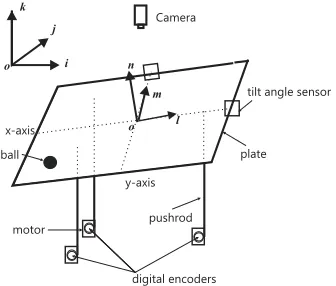
As a representative of a genuine application, a Ball and Plate system has been used for the validation and verification of various advanced multivariable control techniques (Awtar et al., 2002; Castro, Flores, Salton, & Pereira, 2014; Date, Sampei, Ishikawa, & Koga, 2004; Fan, Zhang, & Teng, 2004; Oriolo & Vendittelli, 2005; Wang, Sun, Wang, Liu, & Chen, 2014; Yuan & Zhang, 2010). The entire system model is comprised of three components, which are the Ball and Plate dynamics, the motor dynamics and the push-rod systems which establish the physical relationships between the motors and the plate. In this paper, a novel Ball and Plate system model is devised where three electric motors work cooperatively. Not only can a predefined the ball trajectory on the plate be achieved, but also the ball is maintained at a fixed height. As a consequence, the tilt axes of the plate are always underneath the ball.
The system physical structure is shown in Fig. 1 in which the rotation angles of the motor shafts are measured by the digital encoders. The tilt angles of the plate are measured by two angle sensors and a digital camera sitting above the plate measures the position and velocity of the ball. In contrast to the conventional Ball and Plate system in which only two motors are used to tilt the plate along two orthogonal axes located on the symmetric centre of the plate, here the plate is supported by three vertical pushrods which allow the tilt axis of the plate to remain underneath the rolling ball and therefore the ball will not be launched off the plate in the situation where the distance between the tilt axis and the ball is large. The control objectives are to make the ball roll along a predefined trajectory on the plate whilst maintaining the ball at a fixed datum height. Consider a Ball and Plate system with the kinetic energy
U = 1 2ms˙
2+ 1
2Jbω
2+1
2Jpω
2
p (32)
and the potential energy
T =mgh (33)
For Peer Review
Camera
motor
ball plate
pushrod x-axis
y-axis
digital encoders n
l m i
j k
o o
[image:12.595.216.384.58.201.2]tilt angle sensor
Figure 1. Physical Structure of Ball and Plate System
Then Lagrangian can be written as
L= 1 2ms˙
2+ 1
2Jbω
2+1
2Jpω
2
p−mgh (34)
By letting the plate rotate through θ followed by φ, a mapping between the local and inertial coordinates can be established as
⎡
⎣
ol o m
on
⎤
⎦= ⎡
⎣
cosθ sinθsinφ −sinθcosφ
0 cosφ sinφ
sinθ −cosθsinφ cosθcosφ
⎤
⎦ ⎡
⎣
oi oj ok
⎤
⎦ (35)
where{oi, oj, ok} denotes the inertial coordinate and {ol, o m, on} denotes the local coordinate of the plate or the coordinate of the ball relative to the plate. Suppose the coordinate of the ball relative to the plate is
d=xl+y m+rbn (36)
From (35), the displacement of the ball corresponding to the plate in the inertial coordinate is
s= ¯s1i+ ¯s2j+hk (37)
where
⎡
⎣
¯
s1
¯
s2
h
⎤
⎦= ⎡
⎣
cosθ 0 sinθ
sinθsinφ cosφ −cosθsinφ
−sinθcosφ sinφ cosθcosφ
⎤
⎦ ⎡
⎣
x y rb
⎤
⎦ (38)
From (35) and (37) it follows
˙
s= ( ˙x+rbθ˙−ysinθφ˙)l+ ( ˙y+ ˙φ(xsinθ−rbcosθ))m + (ycosθφ˙−xθ˙)n (39)
Defining an angular velocity coordinate transformation as
⎡
⎣
˜
p
˜
q
˜
r
⎤
⎦= ⎡
⎣
1 0 sinφ
0 cosφ −sinφcosθ
0 sinφ cosθcosφ
⎤
⎦ ⎡
⎣
˙
φ
˙
θ
0
⎤
⎦ (40)
For Peer Review
the angular velocity of the plate relative to the earth can be written as
ωp= ˜pi+ ˜qj+ ˜rj= ˙φi+ cosφθj˙ + sinφθk˙ = cosθφl˙ + ˙θ m+ sinθφn˙ (41)
The angular velocity of the ball relative to the earth is then given by
ω=ωxl+ωym+ωzn+ωp= (ωx+cosθφ˙)l+(ωy+ ˙θ)m+(ωz+sinθφ˙)n (42)
Substituting (38-42) into (34) yields
L=1
2m(( ˙x+rbθ˙−ysinθφ˙)
2+ ( ˙y+ ˙φ(xsinθ−r
bcosθ))2+ (ycosθφ˙−xθ˙)2) +Jb
2((ωx+ cosθφ˙)
2+ (ω
y + ˙θ)2+ (ωz+ sinθφ˙)2) +Jp
2 ((cosθφ˙)
2+ ˙θ2+(sinθφ˙)2)−mg(−xsinθcosφ+ysinφ+r
bcosθcosφ)
(43)
where
Jp = 1 12m(a
2+b2) and J
b = 2 5mr
2
b (44)
The Lagrangian equations with respect to x, y, ωx andωy are given by
d dt(
∂L ∂x˙)−
∂L ∂x =fx
d dt(
∂L ∂y˙)−
∂L
∂y =fy (45)
d dt(
∂L ∂ωx
)− ∂L ∂ψ1
=mωx
d dt(
∂L ∂ωy
)− ∂L ∂ψ2
=mωy (46)
Substituting (43) into (45) and (46) yields
fx=−m(−x−r¨ bθ¨+2 ˙ysinθφ˙+ysinθφ¨+ ˙φ2xsin2θ−sinθφ˙2rbcosθ+xθ˙2+gsinθcosφ) (47)
fy=m(2 ˙φsinθx˙+2 ˙φxcosθθ˙+ 2 ˙φrbsinθθ˙+ ¨φ(xsinθ−rbcosθ) + ¨y−φ˙2y+gsinφ) (48)
mωx =Jb(cosθφ¨−sinθθ˙φ˙+ ˙ωx) (49)
mωy =Jb(¨θ+ ˙ωy) (50)
Since the moments on the ball are produced byfy and fx, it follows
mωx =rbfy and mωy =−rbfx (51)
Using the fact that ¨y =−rbω˙x and ¨x=rbω˙y, and combining (47)-(51) yields
For Peer Review
¨
y=5
7(−2 ˙φsinθx−˙ 2 ˙φxcosθθ−x˙ sinθφ−¨ 12
5 rbφ˙sinθθ˙+ ˙φ
2y−gsinφ)+r
bcosθφ¨ (53)
As defined in Fig. 2, (X1, Y1, Z1), (X2, Y2, Z2) and (X3, Y3, Z3) represent the coordinates of three
points connected to the pushrods. So, by inspecting Figure 3,
-20 -15 -10 -5 0 5 10 15 20 -15
-10 -5 0 5 10 15
Length
Width
(X , Y , Z3 3 3)
(X , Y , Z1 1 1) (X , Y , Z2 2 2)
e
f
Figure 2. Surface of the Plate
z2
z3
(z z1+2)/2
z2
z1
z1
e f
θ
φ
Figure 3. Relationship Between Tilting Angles of Plate and Displacements of Pushrods
θ= arcsinZ3− Z1+Z2
2
e and φ= arcsin
Z2−Z1
f (54)
and ˙θ, ˙φ, ¨θ and ¨φ, derived from (54), are given by
˙
θ= 2 ˙Z3−Z˙1−Z˙2 2ecosθ φ˙=
˙
Z2−Z˙1
fcosφ (55)
¨
θ= 2 ¨Z3−Z¨1−Z¨2 2ecosθ +
( ˙Z3−Z˙1+ ˙2Z2)2(Z3− Z1+2Z2)
e3(cos2θ)3 2
(56)
¨
φ= Z¨2−Z¨1
fcosφ +
( ˙Z2−Z˙1)2(Z2−Z1)
f3(cos2φ)32
(57)
where
cosθ=
1−(Z3− Z1+Z2
2
e )
2 and cosφ=
1−(Z2−Z1
f )
2
As shown in Fig. 4, the motor-pushrod mechanism ensures three push-rods to move vertically. The pushrod is always under compression due to the existence of the spring and therefore any backlash in the motor gears is eliminated. The length of the rod is chosen to be at least ten times that of the motor shaft so that the angle between the connecting rod and the vertical line remains small. Using the small-angle approximation, the vertical displacement of theith push-rod is given by
Zi =lsinαi ∀i= 1 : 3 (58)
For Peer Review
connecting rod unfixed flexible
joint
joint
fixed sleeve spring
supporting plate
motor shaft
α
Figure 4. Motor-Pushrod Mechanism
wherel is the length of the motor shaft,αi is the rotation angle of theith motor shaft. Using the plate surface equation
x−X1 y−Y1 h−Z1
X2−X1 Y2−Y1 Z2−Z1
X3−X1 Y3−Y1 Z3−Z1
= 0 (59)
and substituting (58) into (59), ¨h can be expressed usingx,y, ˙x, ˙y, ¨x, ¨y,αi, ˙αi and ¨αi (i= 1 : 3). Here in this example, the angular accelerations of the plane (i.e. ¨θand ¨φfrom (56) and (57)) and the accelerations of the three pushrods (i.e. ¨αi, i = 1 : 3) cannot be measured straightforwardly. Based upon Kirchhoff’s law, the equation that describes the electric circuit of each armature is
La
dIi
dt +RmIi = ¯Vi−Keα˙i ∀i= 1 : 3 (60)
Clearly from (60), a relationship between current flow into the motor and the angular velocity of the rotor is established. Using the torque balance equation, the angular acceleration of the rotor can be written as
¨
αi=
Kt( ¯Vi−LaI˙i)−(KtKe+Rm˜b) ˙α
JmRm
∀= 1 : 3 (61)
Using the appropriate equations derived above, the full nonlinear Ball and Plate system model can be built. The values of physical parameters used subsequently in this paper are listed in Table 1.
5. Determination of the Desired Eigenstructure
5.1 Selecting the Desired Eigenvector
This section demonstrates how to develop a set of ideal eigenstructure via the analysis of the physical characteristics of Ball and Plate system. Let the model developed in the earlier section be
For Peer Review
Table 1. Model Parameters
Parameter Value Parameter Value
e 0.3(m) ˜b 1.5297(N m/(rad/s))
f 0.2(m) Kt 3 (v/rpm)
rb 0.0175(m) Jm 0.4(kgm2) (X1, Y1) (0.15,−0.1)(m) Ke 4.77(v/rpm) (X2, Y2) (0.15,0.1)(m) Rm 4.7(Ω) (X3, Y3) (−0.15,0)(m) La 0.4(H)
a 0.4(m) b 0.3(m)
l 0.05(m) g 9.81(N m/s2)
be written as
xf ull= [x x y˙ y α˙ 1 α2 α3 α˙1 α˙2 α˙3 I1 I2 I3]T (62)
Due to the fast dynamics of the motor armature currents, their statesI1,I2andI3can be eliminated
from (62). So,
xr=
x x y˙ y α˙ 1 α2 α3 α˙1 α˙2 α˙3
T
(63)
Define a coordinate transformation ˜x → T xr in terms of the mathematical model developed in Section 4, and in the new coordinate, system states are given by
˜
x=
x x y˙ y φ˙ φ θ˙ θ h˙ h˙T
(64)
and system inputs ˜u and outputs ˜y are selected as
˜
u=¯
V1 V¯2 V¯3
T
˜
y=
x y x˙ y φ θ h˙ T (65)
where ¯Vi is from (61). The state space matrices associated with the new coordination system are given in Appendix A.
Remark 5.1: In this special three-motor Ball and Plate system, it is unrealistic the derive the
desired eigenstructure in terms of system states in (63). This is because states x, y, x˙ and y˙ are coupled with states αi and α˙i. In the new coordinate system, the system states in x˜ can be divided
into three groups: (x, x˙, θ,θ˙), (y, y˙, φ, φ˙) and (h, h˙) and each group is decoupled from the rest.
In this paper, the transfer function approach is used to preserve the integral relationships between system states. For the subsystem corresponding to the first group of system states, eigenvalues will be assigned as follows: one complex pair of poles (λx,λ¯x) to determine the second-order response of the position and velocity of the ball, and one complex pair of poles (λθ,λ¯θ) to determine the second-order response of the angular position and angular velocity of the plate. The responses of the position of the ball and the angle of the plate are related to the velocity of the ball and the angular velocity of the plate through integration. Furthermore, based upon the kinematics developed in the earlier section, the mode corresponding to the ball dynamics is not visible in the plate dynamics but the mode corresponding to the plate dynamicsis visible in the ball dynamics.
[image:16.595.107.459.64.184.2]For Peer Review
Therefore the set of transfer functions can be written as
x u1
= 1
(s+λx)(s+ ¯λx)(s+λθ)(s+ ¯λθ) ˙
x u1
= s
(s+λx)(s+ ¯λx)(s+λθ)(s+ ¯λθ)
θ u1
= 1
(s+λθ)(s+ ¯λθ) ˙
θ u1
= s
(s+λθ)(s+ ¯λθ)
(66)
whereu1 denotes the input excitation associated with the subsystem (x, ˙x, θ, ˙θ). Let the
fourth-order subsystem have an input matrixBs= [0 0 0 1]T, an output matrixCs=I4, a modal matrix
denoted by Λs, and let the left and right eigenvectors be denoted byWs andVs, respectively. The transfer function of the subsystem can be written as
Gs(s) =CsVs(sI−Λs)−1WsBs (67)
By definingri as elements of CsVs andti as elements ofWsBs, (67) can be expanded as follows:
⎡ ⎢ ⎢ ⎣ x ˙ x θ ˙ θ ⎤ ⎥ ⎥ ⎦ = ⎡ ⎢ ⎢ ⎣ ¯
r1 r1 r¯5 r5
¯
r2 r2 r¯6 r6
¯
r3 r3 0 0
¯
r4 r4 0 0
⎤ ⎥ ⎥ ⎦ ⎡ ⎢ ⎢ ⎢ ⎣ 1
s+λθ 0 0 0 0 s+ ¯1λ
θ 0 0
0 0 s+1λ x 0 0 0 0 s+ ¯1λ
x ⎤ ⎥ ⎥ ⎥ ⎦ ⎡ ⎢ ⎢ ⎣ ¯ t1 t1 ¯ t2 t2 ⎤ ⎥ ⎥ ⎦
u1 (68)
In (68), null elements appear inCsVs because the modeλx is not visible in θ and ˙θ. From (68),
x u1
= r¯1t¯1
s+λθ
+ r1t1
s+ ¯λθ
+ r¯5t¯2
s+λx
+ r5t2
s+ ¯λx ˙
x u1
= r¯2t¯1
s+λθ
+ r2t1
s+ ¯λθ
+ r¯6t¯2
s+λx
+ r6t2
s+ ¯λx
θ u1
= r¯3t¯1
s+λθ
+ r3t1
s+ ¯λθ ˙
θ u1
= r¯4t¯1
s+λθ
+ r4t1
s+ ¯λθ
(69)
Equating coefficients with the numerators of the ideal transfer functions, the eigenvector elements
For Peer Review
ri (i= 1, . . . ,6),t1 and t2 satisfy
x u1
s3: 0 = ¯r1t¯1+r1t1+ ¯r5t¯2+r5t2 (70)
s2: 0 = ¯r1t¯1(λx+ ¯λx+ ¯λθ) +r1t1(λθ+λx+ ¯λx) + ¯r5t¯2(λθ+ ¯λx+ ¯λθ)
+r5t2(λθ+λx+ ¯λθ) (71)
s1: 0 = ¯r1t¯1( ¯λθλx+ ¯λθλ¯x+λxλ¯x) +r1t1(λθλx+λθλ¯x+ ¯λxλx)
+ ¯r5t¯2(λθλ¯θ+λθλ¯x+ ¯λθλ¯x) +r5t2(λθλ¯θ+λθλx+ ¯λθλx) (72)
s0: 0= ¯r1t¯1λ¯θλxλ¯x+r1t1λθλxλ¯x+ ¯r5t¯2λθλ¯θλ¯x+r5t2λθλ¯θλx (73) ˙
x u1
s3: 0 = ¯r2t¯1+r2t1+ ¯r6t¯2+r6t2 (74)
s2: 0 = ¯r2t¯1(λx+ ¯λx+ ¯λθ) +r2t1(λθ+λx+ ¯λx) + ¯r6t¯2(λθ+ ¯λx+ ¯λθ)
+r6t2(λθ+λx+ ¯λθ) (75)
s1: 0= ¯r2t¯1( ¯λθλx+ ¯λθλ¯x+λxλ¯x) +r2t1(λθλx+λθλ¯x+ ¯λxλx)
+ ¯r6t¯2(λθλ¯θ+λθλ¯x+ ¯λθλ¯x) +r6t2(λθλ¯θ+λθλx+ ¯λθλx) (76)
s0: 0 = ¯r2t¯1λ¯θλxλ¯x+r2t1λθλxλ¯x+ ¯r6t¯2λθλ¯θλ¯x+r6t2λθλ¯θλx (77)
θ u1
s1: 0 = ¯r3t¯1+r3t1 (78)
s0: 0= ¯r3t¯1λ¯θ+r3t1λθ (79)
˙
θ u1
s1: 0= ¯r4t¯1+r4t1 (80)
s0: 0 = ¯r4t¯1λ¯θ+r4t1λθ (81) Note that not all of the above eigenvector elements can be arbitrarily assigned, and the left and right eigenvectors must satisfy
I4 =WsVs (82)
Equation (82) can be converted into the following constraints onri(i= 1, . . . ,6),t1 andt2 as
[0 0 0 1]T =CsVsWsBs (83)
⎡
⎢ ⎢ ⎣
0 0 0 1
⎤
⎥ ⎥ ⎦
=
⎡
⎢ ⎢ ⎣
¯
r1t¯1+r1t1+ ¯r5t¯2+r5t2
¯
r2t¯1+r2t1+ ¯r6t¯2+r6t2
¯
r3t¯1+r3t1
¯
r4t¯1+r4t1
⎤
⎥ ⎥ ⎦
(84)
Examination of (84) shows that the constraints in (70), (74) and (78) are inherently satisfied. To satisfy (81),
r4=
r3
λθ
and r¯4 =
¯
r3
¯
λθ
(85)
which will satisfy equation (78). Substituting (85) into (71) and (72) to eliminate ¯r5r¯2 yields
0 = ¯r1t¯1λx+r1t1λx+r5t2λx−r¯1t¯1λθ−r1t1λ¯θ−r5t2λ¯x (86)
For Peer Review
and
0 = ¯r1t¯1( ¯λθλx+λxλ¯x−λθλ¯θ−λθλ¯θ) +r1t1(λθλx+λxλ¯x−λθλ¯θ−λ¯θλ¯x) +r5r2(λθλx+ ¯λθλx−λθλ¯x−λ¯θλ¯x)
(87)
Substituting (86) into (87) to eliminate r5r2 yields
0 = ¯r1t¯1(λxλ¯x−λθλ¯x−λxλθ+λθλθ) +r1t1(λxλ¯x−λ¯θλ¯x−λxλ¯θ+ ¯λθλ¯θ) (88) From (78) it follows that
r1=
r3
λxλ¯x−λ¯θλ¯x−λ¯θλx+ ¯λθ2 ¯
r1= r¯3
λxλ¯x−λθλ¯x−λθλx+λ2θ
(89)
Substituting (74) into (75) and (77) to eliminate ¯r6t¯2 yields
0 = ¯r2t¯1λx+r2t1λx+r6t2λx−r¯2t¯1λθ−r2t1λ¯θ−r6t2λ¯x (90) and
0 = ¯r2t¯1( ¯λθλxλ¯x−λθλ¯θλ¯x) +r2t1(λθλxλ¯x−λθλ¯θλ¯x) +r6r2(λθλ¯θλx−λθλ¯θλ¯x) (91) Substituting (90) into (91) to eliminate r6r2 yields
0 = ¯r2r¯1( ¯λθλxλ¯x−λθλ¯θλ¯x−λθλ¯θλx+λ2θλ¯θ)+r2r1(λθλxλ¯x−λθλ¯θλ¯x−λθλ¯θλx+λθλ¯θ2) (92) Comparing (78) and (92), r2 can be expressed as
r2 =
r3
λθλxλ¯x−λθλ¯θλ¯x−λθλ¯θλx+λθλ¯θ2 ¯
r2 =
¯
r3
¯
λθλxλ¯x−λθλ¯θλ¯x−λθλ¯θλx+λ2θλ¯θ
(93)
Now substituting (70) into (71) and (72) respectively to eliminate ¯r1t¯1 yields
0 =r1t1(λθλx+λθλ¯x−λ¯θλx−λ¯θλ¯x)+ ¯r5r¯2(λθλ¯θ+λθλ¯x−λ¯θλx−λxλ¯x) +r5r2(λθλ¯θ+λθλx−λ¯θλ¯x−λxλ¯x)
(94)
and
0 =r1t1(λθ−λ¯θ) +r5t2(λθ−λ¯x) + ¯r5r¯2(λθ−λx) (95) After combining (94) and (95) to eliminater1t1, it follows that
0 = ¯r5t¯2(λθλ¯θ−λ¯θλx−λθλx+λ2x) +r5r2(λθλ¯θ−λ¯θλ¯x−λθλ¯x+ ¯λx2) (96)
For Peer Review
Similarly, (74) is substituted into (75) and (77) to eliminate ¯r2t¯1, which yields
0 =r2t1(λθλxλ¯x−λ¯θλxλ¯x)+ ¯r6r¯2(λθλ¯θλ¯x−λ¯θλxλ¯x)+r6r2(λθλ¯θλx−λ¯θλxλ¯x) (97) and
0 =r2t1(λθ−λ¯θ) + ¯r6t¯2(λθ−λx) +r6r2(λθ−λ¯x) (98) Combining (97) and (98) to eliminate r2t1:
0 = ¯r6t¯2(λθλ¯θλ¯x−λ¯θλxλ¯x−λxλ¯xλθ+λ2xλ¯x)+r6r2(λθλ¯θλx−λ¯θλxλ¯x−λxλ¯xλθ+λxλ¯x
2
) (99)
From (96) and (99),r6 and ¯r6 can be expressed byr5 and ¯r5 respectively:
r6 =
r5(λθλ¯θ−λ¯θλ¯x−λθλ¯x+ ¯λx2)
λθλ¯θλx−λ¯θλxλ¯x−λxλ¯xλθ+λxλ¯x2 ¯
r6 = r¯5(λθ
¯
λθ−λ¯θλx−λθλx+λ2x)
λθλ¯θλ¯x−λ¯θλxλ¯x−λxλ¯xλθ+λ2xλ¯x
(100)
For the second group of states (y,y, θ,˙ θ˙), the desired closed-loop eigenvectors can be developed simply by replacingλx,λθ in (85-100) with λy, λφ.
For the third group of states, ˙h and h, let the second-order subsystem have an input matrix [0 1]T and define r7 and r8 as the elements of the corresponding eigenvectors. The subsystem
transfer function matrix can then be expressed as
h
˙
h =
¯
r7 r7
¯
r8 r8
1
s+λh 0 0 s+ ¯1λ
h
¯
t3
t3 u3 (101)
whereu3 denotes the input excitation associated with the subsystem (h, ˙h). From (101),
h u3
= r¯7t¯3
s+λh
+ r7t3
s+ ¯λh ˙
h u3
= r¯8t¯3
s+λh
+ r8t3
s+ ¯λh
(102)
After equating coefficients with the numerators of the ideal transfer functions, the eigenvector elements r7,r8, ¯t3 and t3 satisfy
h u3
s1 : 0 = ¯r7t¯3+r7t3 (103)
s0 : 0= ¯r7t¯3λ¯h+r7t3λh (104) ˙
h u3
s1 : 0= ¯r8t¯3+r8t3 (105)
s0 : 0 = ¯r8t¯3λ¯h+r8t3λh (106) Comparing (103) and (106) yields
r8=
r7
λh
and r¯8 =
¯
r7
¯
λh
(107)
For Peer Review
Since only the directions of eigenvectors are crucial for the design purpose,r3,r5and r7 are
nor-malized to unity for convenience. After combining (85), (89), (93), (100) and (107), the complete set of ideal closed-loop eigenvectors for the system, which is consistent with the original requirements, is given by
⎡ ⎢ ⎢ ⎢ ⎢ ⎢ ⎢ ⎢ ⎢ ⎢ ⎢ ⎢ ⎢ ⎢ ⎢ ⎣ x ˙ x y ˙ y φ ˙ φ θ ˙ θ h ˙ h ⎤ ⎥ ⎥ ⎥ ⎥ ⎥ ⎥ ⎥ ⎥ ⎥ ⎥ ⎥ ⎥ ⎥ ⎥ ⎦ ∼ ⎡ ⎢ ⎢ ⎢ ⎢ ⎢ ⎢ ⎢ ⎢ ⎢ ⎢ ⎢ ⎢ ⎢ ⎣
1 1 0 0 0 0 c¯6 c6 0 0
¯
c1 c1 0 0 0 0 c¯7 c7 0 0
0 0 1 1 c¯3 c3 0 0 0 0
0 0 c¯2 c2 c¯4 c4 0 0 0 0
0 0 0 0 1 1 0 0 0 0
0 0 0 0 c¯5 c5 0 0 0 0
0 0 0 0 0 0 1 1 0 0
0 0 0 0 0 0 c¯8 c8 0 0
0 0 0 0 0 0 0 0 1 1
0 0 0 0 0 0 0 0 c¯9 c9
⎤ ⎥ ⎥ ⎥ ⎥ ⎥ ⎥ ⎥ ⎥ ⎥ ⎥ ⎥ ⎥ ⎥ ⎦ (108)
where∼denotes correspondence between states and matrix rows and
c1 =
λθλ¯θ−λ¯θλ¯x−λθλ¯x+ ¯λx2
λθλ¯θλx−λ¯θλxλ¯x−λxλ¯xλθ+λxλ¯x2
c2 =
λφλ¯φ−λ¯φλ¯y−λφλ¯y+ ¯λy2
λφλ¯φλy−λ¯φλyλ¯y−λyλ¯yλφ+λyλ¯y2
c3 =
1
λyλ¯y−λ¯φλ¯y−λ¯φλy+ ¯λφ2
c4 =
1
λφλyλ¯y−λφλ¯φλ¯y−λφλ¯φλy+λφλ¯φ2
c5 =
1
λφ
c6 =
1
λxλ¯x−λ¯θλ¯x−λ¯θλx+ ¯λθ
2
c7 =
1
λθλxλ¯x−λθλ¯θλ¯x−λθλ¯θλx+λθλ¯θ
2
c8 =
1
λθ
c9 =
1
λh
(109)
5.2 Defining Ideal Eigenvalues
The damping ratios of all system eigenvalues/modes are assumed to be 0.8. In the Ball and Plate system, both the ball and the plate dynamics are slower than those of the three motors, and the settling times of the modes corresponding to the tilt angles of the plate are assumed to be faster than the mode associated with the ball position. By increasing the settling time of the tilt angles of the plate, the control effort is reduced and the movement of the plate becomes smoother. Furthermore, in order to maintain the ball at a fixed height, the mode associated with the ball height is assumed to be faster than those associated with the tilt angles of the plate. The set of
For Peer Review
desired eigenvalues in continuous-time is
{λx,λ¯x}=−0.8±0.6i
{λy,λ¯y}=−0.6±0.45i
{λφ,λ¯φ}=−5±4i (110)
{λθ,λ¯θ}=−4.5±3.6i
{λh,λ¯h}=−15±12i
6. Application of Multistage Output-Lifting Eigenstructure Assignment
The Ball and Plate system is a typical multirate output feedback control system. Sensors and actuators around the system operating at different sampled rates. The camera samples the ball position and velocity every 40ms. The tilt angles of the plate are measured by digital encoders which operate every 10ms. The height of the ball is calculated using hardware logic with the sampling interval chosen to be 10ms. The DC motors are driven by PWM signals with a frame rate of 40ms. From (64-65), m = 7, n = 10, r = 3. It is not straightforward to fully assign a desired eigenstructure using a traditional output feedback EA framework becausem+r =n. So, let the main sampling period be 40ms and the base sampling period be 10ms. Then the desired discrete-time eigenvalues associated with ˜x, discretized using the main sampling period 40ms, are
Λd=diag([λdx λ¯dx λdy λ¯dy λdφ λ¯dφ λdθ λ¯dθ λdh λ¯dh]) (111)
where
{λdx,λ¯dx}= 0.9682±0.0232i
{λdy,λ¯dy}= 0.9761±0.0176i
{λdφ,λ¯dφ}= 0.8083±0.1304i (112)
{λdθ,λ¯dθ}= 0.8266±0.1199i
{λdh,λ¯dh}= 0.4868±0.2534i
The desired left and right eigenvectors can be calculated by substituting desired continuous-time eigenvalues (110) into (108). The values of desired eigenvectors will be illustrated later in the paper. In this section, multistage output feedback EA is applied to Ball and Plate system. In the first stage, thes1 = 8 eigenpairs (s2 < n−1) associated with λx,λy,λφand λθ are assigned using the right allowable subspace. In the second stage, the remainings2 = 2 eigenparis (s2≤r) associated
with λh are assigned using the left allowable subspace. As argued in Section 4, the eigenvectors assigned from the left allowable subspace should be improved compared with those assigned via full state feedback EA and conventional output-lifting EA.
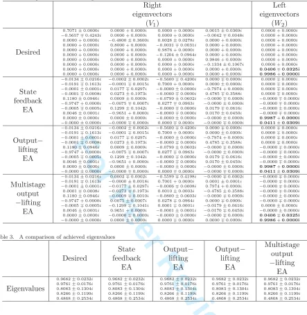
To show the efficacy of the scheme, the desired left and right eigenvectors and those achieved using single rate full state feedback EA (G. P. Liu & Patton, 1998; White, 1995), output-lifting EA (L. Chen et al., 2017) and multistage output-lifting EA are presented in this section. The comparison results are shown in Table. 2. where it can be seen (in particular the bold part) that the left eigenvectors, assigned using state feedback EA and conventional output-lifting EA, can be further improved via multistage output-lifting EA and the desired left eigenvectors can be exactly assigned. In addition, the right eigenvectors, assigned (in the first stage) via full state feedback EA, output-lifting EA and proposed multistage output-lifting EA, are the same due to the invariance of the dimension of the right allowable subspace.
For Peer Review
Table 2. A comparison of achieved eigenvectors
Right Left
eigenvectors eigenvectors
(V1) (W2)
Desired
0.7071±0.0000i 0.0000 + 0.0000i 0.0000 + 0.0000i 0.0015±0.0369i −0.5657∓0.4243i 0.0000 + 0.0000i 0.0000 + 0.0000i −0.0042∓0.0048i
0.0000 + 0.0000i −0.4800±0.3600i 0.0028±0.0278i 0.0000 + 0.0000i 0.0000 + 0.0000i 0.8000 + 0.0000i −0.0031∓0.0031i 0.0000 + 0.0000i 0.0000 + 0.0000i 0.0000 + 0.0000i 0.9876 + 0.0000i 0.0000 + 0.0000i 0.0000 + 0.0000i 0.0000 + 0.0000i −0.1204±0.0964i 0.0000 + 0.0000i 0.0000 + 0.0000i 0.0000 + 0.0000i 0.0000 + 0.0000i 0.9846 + 0.0000i 0.0000 + 0.0000i 0.0000 + 0.0000i 0.0000 + 0.0000i −0.1334±0.1067i 0.0000 + 0.0000i 0.0000 + 0.0000i 0.0000 + 0.0000i 0.0000 + 0.0000i 0.0000 + 0.0000i 0.0000 + 0.0000i 0.0000 + 0.0000i 0.0000 + 0.0000i
0.0000 + 0.0000i 0.0000 + 0.0000i 0.0000 + 0.0000i 0.0000 + 0.0000i 0.0000 + 0.0000i 0.0000 + 0.0000i 0.0000 + 0.0000i 0.0000 + 0.0000i
0.0406∓0.0325i 0.9986+0.0000i
State feedback
EA
−0.0134±0.0216i −0.0002±0.0002i −0.5600∓0.4200i 0.0000∓0.0000i −0.0191∓0.1613i −0.0001∓0.0015i 0.7000 + 0.0000i 0.0000±0.0000i −0.0001±0.0001i 0.0177∓0.0297i −0.0000±0.0000i −0.7974 + 0.0000i −0.0001∓0.0008i 0.0273±0.1973i −0.0000∓0.0000i 0.4785∓0.3588i
0.1180±0.0946i 0.0009±0.0009i −0.0799±0.0602i −0.0000∓0.0000i −0.9747 + 0.0000i −0.0075∓0.0007i 0.0277∓0.0963i −0.0000±0.0000i −0.0005∓0.0005i 0.1299±0.1042i −0.0000∓0.0000i 0.0179∓0.0616i
0.0046±0.0001i −0.9651 + 0.0000i −0.0000∓0.0000i 0.0170±0.0450i 0.0000±0.0000i 0.0000±0.0000i −0.0000±0.0000i −0.0000±0.0000i −0.0000±0.0000i −0.0000∓0.0000i 0.0000∓0.0000i −0.0000∓0.0000i
0.0000∓0.0000i 0.0000∓0.0000i 0.0000∓0.0000i 0.0000∓0.0000i −0.0000∓0.0000i −0.0000∓0.0000i −0.0000±0.0000i −0.0000∓0.0000i
0.9987+0.0000i 0.0411±0.0309i
Output−
lifting EA
−0.0134±0.0216i −0.0002±0.0002i −0.5600∓0.4200i 0.0000∓0.0000i −0.0191∓0.1613i −0.0001∓0.0015i 0.7000 + 0.0000i 0.0000±0.0000i −0.0001±0.0001i 0.0177∓0.0297i −0.0000±0.0000i −0.7974 + 0.0000i −0.0001∓0.0008i 0.0273±0.1973i −0.0000∓0.0000i 0.4785∓0.3588i
0.1180±0.0946i 0.0009±0.0009i −0.0799±0.0602i −0.0000∓0.0000i −0.9747 + 0.0000i −0.0075∓0.0007i 0.0277∓0.0963i −0.0000±0.0000i −0.0005∓0.0005i 0.1299±0.1042i −0.0000∓0.0000i 0.0179∓0.0616i
0.0046±0.0001i −0.9651 + 0.0000i −0.0000∓0.0000i 0.0170±0.0450i 0.0000±0.0000i 0.0000±0.0000i −0.0000±0.0000i −0.0000±0.0000i −0.0000±0.0000i −0.0000∓0.0000i 0.0000∓0.0000i −0.0000∓0.0000i
0.0000∓0.0000i 0.0000∓0.0000i 0.0000∓0.0000i 0.0000∓0.0000i −0.0000∓0.0000i −0.0000∓0.0000i −0.0000±0.0000i −0.0000∓0.0000i
0.9987+0.0000i 0.0411±0.0309i
Multistage output
−lifting EA
−0.0134±0.0216i 0.0002∓0.0002i −0.5599∓0.4198i −0.0000∓0.0002i −0.0191∓0.1613i −0.0000±0.0018i 0.7001 + 0.0000i 0.0001±0.0001i −0.0001±0.0001i −0.0177±0.0297i −0.0006∓0.0008i 0.7974 + 0.0000i 0.0001∓0.0008i −0.0273∓0.1973i 0.0010±0.0003i −0.4785±0.3588i 0.1180±0.0946i −0.0009∓0.0010i −0.0800±0.0603i −0.0000∓0.0000i −0.9747 + 0.0000i 0.0075±0.0007i 0.0278∓0.0964i 0.0000∓0.0000i −0.0005∓0.0005i −0.1299∓0.1041i 0.0001∓0.0001i −0.0179±0.0616i
0.0046±0.0001i 0.9651 + 0.0000i −0.0001±0.0001i −0.0170∓0.0450i 0.0000±0.0000i −0.0000∓0.0000i −0.0000±0.0000i −0.0000∓0.0000i −0.0000±0.0000i 0.0000±0.0000i 0.0000∓0.0000i 0.0000∓0.0000i
−0.0000∓0.0000i −0.0000∓0.0000i −0.0000∓0.0000i −0.0000∓0.0000i −0.0000±0.0000i −0.0000∓0.0000i 0.0000±0.0000i −0.0000±0.0000i
0.0406∓0.0325i 0.9986+0.0000i
Table 3. A comparison of achieved eigenvalues
Desired State feedback EA Output− lifting EA Output− lifting EA Multistage output −lifting EA Eigenvalues
0.9682±0.0232i 0.9761±0.0176i 0.8083±0.1304i 0.8266±0.1199i 0.4868±0.2534i
0.9682±0.0232i 0.9761±0.0176i 0.8083±0.1304i 0.8266±0.1199i 0.4868±0.2534i
0.9682±0.0232i 0.9761±0.0176i 0.8083±0.1304i 0.8266±0.1199i 0.4868±0.2534i
0.9682±0.0232i 0.9761±0.0176i 0.8083±0.1304i 0.8266±0.1199i 0.4868±0.2534i
0.9682±0.0232i 0.9761±0.0176i 0.8083±0.1304i 0.8266±0.1199i 0.4868±0.2534i
It is also clear from Table. 3, multistage output-lifting EA has the capability to assign the desired eigenvalues as those assigned via full state feedback EA.
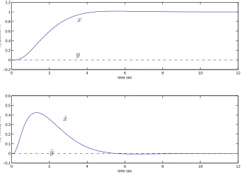
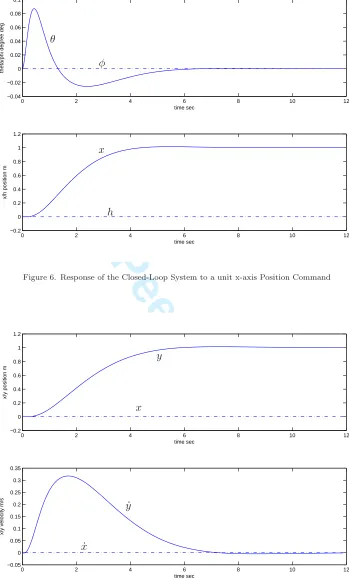
The closed-loop system responses are shown in Figures 5 to 8. Figure 5 shows the position and the velocity responses of the ball along the x- and y-axes, to a unit step reference command along the x-axis. The plots exhibit the desired second-order characteristics, which are compatible with the predefined system modes, and the settling time of the x-position is close to 5sec(4/0.8). Figure 6 shows the angular position and velocity responses of the plant along the x- and y-axis following a unit step reference command along the x-axis. It also shows the height of the ball following a unit step reference command along the x-axis. It is clear that the height of the ball is maintained at a constant, zero-error value. Figure 7 shows the position and the velocity responses of the ball along the x- and y-axes, to a unit step reference command along the y-axis. The second-order response of the y-position is shown to be as required. The settling time is close to 6.6sec(4/0.6). Figure 8 depicts the angle and angular velocity responses of the plant along the x-axis and the y-axis
[image:23.595.78.521.64.522.2] [image:23.595.75.518.66.520.2]For Peer Review
appropriate system modes are well decoupled. Furthermore, the system outputs are able to track given reference commands.
7. Conclusions
In this paper, a multistage output-lifting EA scheme is developed. Compared with conventional output-lifting EA, the left allowable subspace is exploited in this scheme, which allows eigenvector assignment to be further improved. In addition, the mathematical model of a novel Ball and Plate system is developed. Based upon the physical characteristics of the system, an ideal eigenstructure is derived, which allows natural modes to be distributed and decoupled in appropriate states or outputs. Since Ball and Plate is a typical multirate output feedback system with restricted DoF, it is an ideal candidate to apply a multistage output-lifting EA scheme. The design and simulation results show the efficacy of the scheme.
Appendix. A
The Linearized three-motor Ball and Plate system
In the coordination system associated with (64) and (65), the continuous-time state space ma-trices of the three motor Ball and Plate system are
Ac =
⎡
⎢ ⎢ ⎢ ⎢ ⎢ ⎢ ⎢ ⎢ ⎢ ⎢ ⎢ ⎢ ⎢ ⎣
0 1.0000 0 0 0 0 0 0 0 0
0 0 0 0 7.0000 0.2001 0 0 0 0
0 0 0 1 0 0 0 0 0 0
0 0 0 0 0 0 −7 −0.2001 0 0
0 0 0 0 0 1 0 0 0 0
0 0 0 0 0 −11.4360 0 0 0 0
0 0 0 0 0 0 0 1 0 0
0 0 0 0 0 0 0 −11.4360 0 0
0 0 0 0 0 0 0 0 0 1
0 0 0 0 0 0 0 0 0 −11.4360
⎤
⎥ ⎥ ⎥ ⎥ ⎥ ⎥ ⎥ ⎥ ⎥ ⎥ ⎥ ⎥ ⎥ ⎦
(113)
Bc =
⎡
⎢ ⎢ ⎢ ⎢ ⎢ ⎢ ⎢ ⎢ ⎢ ⎢ ⎢ ⎢ ⎢ ⎣
0 0 0
0.0023 0.0023 −0.0047
0 0 0
−0.0070 0.0070 0
0 0 0
−0.1330 −0.1330 0.2660
0 0 0
−0.3989 0.3989 0
0 0 0
0.0199 0.0199 0.0399
⎤
⎥ ⎥ ⎥ ⎥ ⎥ ⎥ ⎥ ⎥ ⎥ ⎥ ⎥ ⎥ ⎥ ⎦
(114)
References
Alireza, E. A., & Batool, L. (2012). Application of matrix perturbation theory in robust control of large-scale systems. Automatica, 48, 1868–1873.
Andry, A. N., Shapiro, E. Y., & Chung, J. C. (1983). Eigenstructure assignment for linear systems. IEEE Trans. Aerosp. Electron. Syst.,19, 711-727.
Awtar, S., Bernard, C., Boklund, N., Master, A., Ueda, D., & Craig, K. (2002). Mechatronic design of a ball-on-plate balancing system. Mechatronics, 12, 217 - 228.
For Peer Review
Castro, R., Flores, J. V., Salton, A. T., & Pereira, L. F. A. (2014, August). A comparative analysis of repetitive and resonant controllers to a servo-vision ball and plate system. InProc. 19th IFAC World Congress. Cape Town, South Africa.
Chen, B., & Nagarajaiah, S. (2007). Linear-matrix-inequality-based robust fault detection and isolation using the eigenstructure assignment method. AIAA Journal of Guidance, Control and Dynamics,30, 1831-1835.
Chen, L., Pomfret, A., & Clarke, T. (2017). Increasing eigenstructure assignment design degree of freedom using lifting. Int. J. Control,90, 2111-2123.
Chen, T., & Francis, B. A. (1995). Optimal sampled-data control systems. Springer, London.
Clarke, T., Ensor, J. E., & Griffin, S. J. (2003). Desirable eigenstructure for good short-term helicopter handing qualities: the attitude command response case. Proceedings of the Institution of Mechanical Engineers, Part G: Journal of Aerospace Engineering,217, 43-45.
Clarke, T., & Griffin, S. J. (2004). An addendum to output feedback eigenstructure assignment:retro-assignment. Int. J. Control, 77, 78-85.
Clarke, T., Griffin, S. J., & Ensor, J. E. (2003). Output feedback eigenstructure assignment using a new reduced orthogonality condition. Int. J. Control,77, 390-402.
Date, H., Sampei, M., Ishikawa, M., & Koga, M. (2004). Simultaneous control of position and orientation for ball-plate manipulation problem based on time-state control form.IEEE T. Robotic. Autom.,20, 465-480.
Duval, C., Clerc, G., & LeGorrec, Y. (2006). Induction machine control using robust eigenstructure assign-ment. Control Eng. Pract.,14, 26-43.
Fahmy, M. M., & O’Reilly, J. (1988). Multistage parametric eigenstructure assignment by output-feedback control. Int. J. Control,48, 97-116.
Fan, X., Zhang, N., & Teng, S. (2004). Trajectory planning and tracking of a ball and plate system using a hierarchical fuzzy control scheme. Fuzzy Sets Syst.,144, 297-312.
Farineau, J. (1989, December). Lateral electric flight control laws of civil aircraft based on eigenstructure assignment technique. In Proc. AIAA Guidance, Navigation and Control Conference. Boston, MA. USA.
Garrard, W. L., Low, E., & Prouty, S. (1989). Design of attitude and rate command systems for helicopters using eigenstructure assignment. AIAA Journal of Guidance, Control and Dynamics,12, 783-791. Kimura, H. (1975). Pole assignment by gain output feedback. IEEE Trans. Autom. Control,20, 509-516. Kimura, H. (1977). A further result on the problem of pole assignment by output feedback. IEEE Trans.
Autom. Control,25, 458-463.
Kshatriya, N., Annakkage, U. D., Hughes, F. M., & Gole, A. M. (2007). Optimized partial eigenstructure assignment-based design of a combined PSS and active damping controller for a DFIG. IEEE Trans. Power Syst.,25, 866–876.
Lhachemi, H., Saussie, D., & Zhu, G. (2017). Explicit hidden coupling terms handling in gain-scheduling control design via eigenstructure assignment. Control Eng. Pract.,58, 1-11.
Liu, G. P., & Patton, R. J. (1998).Eigenstructure assignment for control system design. Wiley, Chichester. Liu, Y., Tan, D. L., Wang, B., & Wang, X. (2013). Linear-matrix-inequality-based fault diagnosis for gas
turbofan engine using eigenstructure assignment principle. Applied Mechanics and Materials, 302, 759–764.
Low, E., & Garrard, W. L. (1993). Design of flight control systems to meet rotorcraft handling qualities specifications. AIAA Journal of Guidance, Control and Dynamics,16, 69-78.
Moore, B. C. (1976). On the flexibility offered by state feedback in multivariable systems beyond closed loop eigenvalue assignment. IEEE Trans. Autom. Control,21, 689-692.
Ntogramatzidis, L., Nguyen, T., & Schmid, R. (2015). Repeated eigenstructure assignment for controlled invariant subspaces. European Journal of Control,26, 1-11.
Oriolo, G., & Vendittelli, M. (2005). A framework for the stabilization of general nonholonomic systems with an application to the plate-ball mechanism. IEEE Trans. Rob., 21, 162-175.
Ouyang, H., Richiedei, D., Trevisani, A., & Zanardo, G. (2012). Discrete mass and stiffness modifications for the inverse eigenstructure assignment in vibrating systems: Theory and experimental validation.
Int. J. Mech. Sci.,64, 211–220.
For Peer Review
Piou, J., & Sobel, K. M. (1994). Yaw pointing and lateral translation using robust sampled data eigenstruc-ture assignment. AIAA Journal of Guidance, Control and Dynamics,17, 1133-1135.
Piou, J., & Sobel, K. M. (1995). Robust multirate eigenstructure assignment with flight control application.
AIAA Journal of Guidance, Control and Dynamics,18, 539-546.
Pomfret, A. J., & Clarke, T. (2009). Desirable eigenstructure for good short-term helicopter handling qualities: the rate command response case. Proceedings of the Institution of Mechanical Engineers, Part G: Journal of Aerospace Engineering,223, 1059-1065.
Pomfret, A. J., Clarke, T., & Ensor, J. (2005, July). Eigenstructure assignment for semi-proper systems: pseudo-state feedback. InProc. 16th IFAC World Congress, Prague.
Roppenecker, G., & O’Reilly, J. (1989). Parametric output feedback controller design. Automatica, 25, 259-265.
Srinathkumar, S. (1978). Eigenvalue/eigenvector assignment using output feedback. IEEE Trans. Autom. Control,23, 79-81.
Wahrburg, A., & Adamy, J. (2013). Parametric design of robust fault isolation observers for linear non-square systems. Systems & Control Letters,62, 420–429.
Wang, Y., Sun, M., Wang, Z., Liu, Z., & Chen, Z. (2014). A novel disturbance-observer based friction compensation scheme for ball and plate system. ISA Transactions,53, 671 - 678.
White, B. A. (1995). Eigenstructure assignment: a survey. Proceedings of the Institution of Mechanical Engineers, Part I: Journal of Systems and Control Engineering,209, 1-11.
White, B. A., Bruyere, L., & Tsourdos, A. (2007). Missile autopilot design using quasi-LPV polynomial eigenstructure assignment. IEEE Trans. Aerosp. Electron. Syst.,43, 1470-1483.
Yuan, D., & Zhang, Z. (2010). Modelling and control scheme of the ball-plate trajectory-tracking pneumatic system with a touch screen and a rotary cylinder. IET Control Theory & Applications, 4, 573-589. Zhao, L., & Lam, J. (2016a). Dominant pole and eigenstructure assignment for positive systems with state
feedback. Int. J. Syst. Sci.,47, 2901-2912.
Zhao, L., & Lam, J. (2016b). Multiobjective controller synthesis via eigenstructure assignment with state feedback. Int. J. Syst. Sci.,47, 3219-3231.
0 2 4 6 8 10 12
−0.2 0 0.2 0.4 0.6 0.8 1 1.2
time sec
x/y position m
0 2 4 6 8 10 12
−0.1 0 0.1 0.2 0.3 0.4 0.5 0.6
time sec
x/y velocity m/s
x
y
˙
x
˙
[image:26.595.127.473.413.673.2]y
Figure 5. Response of the Closed-Loop System to a unit x-axis Position Command
For Peer Review
0 2 4 6 8 10 12
−0.04 −0.02 0 0.02 0.04 0.06 0.08 0.1
time sec
theta/phi degree deg
0 2 4 6 8 10 12
−0.2 0 0.2 0.4 0.6 0.8 1 1.2
time sec
x/h position m
x
h θ
φ
Figure 6. Response of the Closed-Loop System to a unit x-axis Position Command
0 2 4 6 8 10 12
−0.2 0 0.2 0.4 0.6 0.8 1 1.2
time sec
x/y position m
0 2 4 6 8 10 12
−0.05 0 0.05 0.1 0.15 0.2 0.25 0.3 0.35
time sec
x/y velocity m/s
x y
˙
y
˙
x 1
[image:27.595.122.471.88.675.2]For Peer Review
0 2 4 6 8 10 12
−0.06 −0.05 −0.04 −0.03 −0.02 −0.01 0 0.01 0.02
time sec
theta/phi degree deg
0 2 4 6 8 10 12
−0.2 0 0.2 0.4 0.6 0.8 1 1.2
time sec
y/h position m
h y θ
φ
Figure 8. Response of the Closed-Loop System to a unit y-axis Position Command
For Peer Review
Response to the first reviewer:
`I note that a new section (Section 3) is added to this revised paper. In the added section, a two-stage output-lifting eigenstructure assignment approach is proposed. The result can be seen as an extension of the recent work published by L. Chen et al. (2017). However, I have the following concern that the authors should make it clearer.
The authors say that “Instead of only using the right allowable subspace, the left allowable subspace, with an increased dimension induced by output-lifting, will be used to improve the assigned eigenvectors.” The authors should explain the advantages of doing this. Since pm>=n, both the right s_1 eigenpairs and the remaining right s_2 eigenpairs can be easily assigned only using the right allowable subspace. Thus, the authors should clearly explain why assigning the left s_2 eigenpairs via the left allowable subspace can improve the assigned eigenvectors, but assigning the right s_2 eigenpairs via the right allowable subspace cannot improve or can improve less.'
Thanks for the comments. In the modified paper, the discussion of advantages has been expanded and added in the introduction.
‘Although output-lifting allows full state feedback eigenstructure to be assigned from the right allowable subspace, an exact assignment of desired eigenvectors (i.e. assignment of all elements of each eigenvector) is difficult to be achieved due to the limited dimension of the allowable right subspace determined by the number of system inputs. Since output-lifting only enlarges the effective number of system outputs, the dimension of the right allowable subspace is invariant. If only the right allowable subspace is used for eigenvector assignment, the maximum number of exactly assignable elements of each eigenvector, which equates to the number of system inputs, cannot be enlarged anymore. Exploiting the fact that output-lifting has the capability to enlarge the number of effective system outputs, the dimension of the left allowable subspace is thus increased. If the dimension of the left allowable subspace becomes larger than one of the right allowable subspace after output-lifting, a left allowable subspace based eigenvector assignment can further improve achieved eigenvectors and allows more elements of each eigenvector to be exactly assigned. Instead of only using the right allowable subspace for eigenvector assignment (the maximum number of exactly assignable elements of each eigenvector equates to the number of system inputs), this paper developed a multistage output-lifting EA scheme in which both the left and right allowable subspaces are used for EA. In the second stage where the left allowable subspace is used for eigenvector assignment, the partially assigned eigenvectors should contain more elements of desired eigenvectors due to output-lifting. ‘
Additionally, Remarks 2.1 and 3.1 have been expanded to make the explanation clear.