ANN-derived equation and ITS application in the prediction of dielectric properties of pure and impure CO₂

This is a repository copy of ANN-derived equation and ITS application in the prediction of

dielectric properties of pure and impure CO₂.

White Rose Research Online URL for this paper:

http://eprints.whiterose.ac.uk/141611/

Version: Accepted Version

Article:

Abidoye, LK, Mahdi, FM orcid.org/0000-0002-3046-4389, Idris, MO et al. (2 more authors)

(2018) ANN-derived equation and ITS application in the prediction of dielectric properties

of pure and impure CO . Journal of Cleaner Production, 175. pp. 123-132. ISSN

₂

0959-6526

https://doi.org/10.1016/j.jclepro.2017.12.013

© 2017 Elsevier Ltd. All rights reserved. Licensed under the Creative Commons

Attribution-Non Commercial No Derivatives 4.0 International License

(https://creativecommons.org/licenses/by-nc-nd/4.0/).

[email protected] https://eprints.whiterose.ac.uk/ Reuse

This article is distributed under the terms of the Creative Commons Attribution-NonCommercial-NoDerivs (CC BY-NC-ND) licence. This licence only allows you to download this work and share it with others as long as you credit the authors, but you can’t change the article in any way or use it commercially. More

information and the full terms of the licence here: https://creativecommons.org/licenses/ Takedown

If you consider content in White Rose Research Online to be in breach of UK law, please notify us by

ANN-Derived Equation and its Application in the Prediction of Dielectric Properties of

Pure and Impure CO2

Abidoye, L.K.,(1)* _{Mahdi, F.M.,}(2)

, Idris, M.O.(3), Alabi, O.O.(4), W ahab, A.A.(5)

(1) _{Civil Engineering Department, Osun State University, Osogbo, Nigeria.}

(2) _{Chemical Engineering Department, Leeds University, Leeds, UK}

(3) _{Mechanical Engineering Department, Osun State University, Nigeria}

(4) _{Department of Physics, Osun State University, Osogbo, Nigeria.}

(5) _{Department ofBiologicalSciences, Osun State University, Osogbo, Nigeria}

*Corresponding author: +2348054859860, Email: [email protected]

[email protected]

Abstract

High-performing equation has been step-wisely extracted from artificial neural network

(ANN) simulation and subsequently applied for the prediction of the dielectric properties of

pure and impure CO2. Data of relative permittivity ( r) for pure and impure CO2 were used in

the ANN to train different ANN structures so that the network can recognise and predict

CO2 property under different conditions. Analyses of the results from the training showed

that single-layer ANN model [3-6-1] outperformed others. From this best-performing ANN

structure, a single mathematical equation was extracted that can be employed in predicting

r for pure CO2 and CO2-ethanol mixture, even without access to ANN software. Using this

ANN-based mathematical model, predictions of the relative permittivity ( r) for pure CO2 and

CO2-ethanol mixture were performed, under different temperatures and pressures and at

different ethanol concentrations. Under similar conditions, the output of the model provides

good match with the original experimental r. W ith increment in ethanol concentration, the

model correctly predicted the rise in r for the mixture. Also, it was shown that the r rises

reliability and applicability of the ANN in characterizing and predicting the dielectric property

of pure CO2 as well as its mixture or impurities. The model developed and the techniques

demonstrated in this work offers immense benefits and guides for researchers, who may

want to explore the behaviours of a pure compound and its mixtures/impurities using ANN,

as well as those interested in derived mathematical model from statistical computation tool

like ANN.

Keywords: CO2, Relative Permittivity, ANN, Ethanol, Model, Sequestration

NOMENCLATURE

Symbol Description

W Weight assigned by the network

b Bias assigned by the network

Mass fraction of ethanol

T Temperature

P Pressure

r Relative permittivity

X Actual value of parameter of interest

y Normalised value of parameter ‘X’

E Sum of the transformed weighted normalised variables for each neuron in a layer

F Tansig-transformed ‘E’ for each neuron in a layer

AARE Average absolute relative error

SSE Sum Squared Error

NS Nash-Sutcliffe efficiency coefficient

MSE Mean Squared Error

Scal Predicted or calculated value

Sobs Observed or target value

obs

S Average of the observed output

N Total number of data points

n Sequential Count of variable

NI Number of neurons in the first hidden layer

N2 Number of neurons in the second hidden layer

I layer of the network

i neuron in a network (first count)

1. Introduction

Currently, there are ever-growing interests in the properties and applications of carbon

dioxide (CO2), both in the research fields as well as industry. Supercritical carbon dioxide

(scCO2) has the advantages of having low critical temperature and pressure. These qualities

can be easily manipulated to desired ends for research and industrial production. Its

research and industrial prospects are further enhanced by its non-toxicity, non-flammability

and high purity at low cost, which promotes its use in extraction processes that utilize

supercritical fluids (Astray et al. 2012).

On the other hand, CO2 emission has been considered as a major contributor to the global

warming phenomenon (Abidoye et al. 2015; Abidoye and Das 2014a; Abidoye and Das

2015). From different emission sources, CO2 and other greenhouse gases migrate to the

lower atmosphere and form a blanket that reflects heat radiation back to the earth, resulting

in a global rise in temperature across the surface of the earth. Different measures have been

taken by stakeholders to check the increasing accumulation of CO2 in the atmosphere.

Popular measures involve the capture of CO2 from emission sources and the subsequent

injection into the deep geological media (Bielinski et al. 2008), especially in saline aquifer

(Chadwick et al. 2008).

Understanding the properties of CO2 will promote its use in industrial extraction and

research. Understanding these properties can be enhanced using, for example, electrical

conductivity and relative permittivity techniques. The relative permittivity ( r) is a measure of

the electrical polarization of the material (Mahmood et al. 2012) that takes place when an

electric field is applied, while the electrical conductivity ( ), is a measure of the conduction

current resulted from an electric field through the material (see, e.g., Solymar et al. 2014;

Keller 1966). The unique polarization effect of electrical signal on materials, measured as

(2017), Abidoye and Das (2015), Abidoye and Bello (2017)), etc., used the technique of

relative permittivity to determine the quantity of water and/or gas in the porous media.

The ability to predict important properties of CO2 will further enhance its monitoring and

control in geological carbon sequestration. For example, fear has been raised over the

likelihood of leakage of CO2 from geological carbon sequestration site (Abidoye and Das

2014a; Abidoye et al. 2015; Das et al. 2014; Little and Jackson, 2010; Schwartz 2014). As a

result, a number of approaches have been developed to counteract the possibility of

leakage. These include time lapse satellite imaging (Mathieson et al. 2009), wave speeds

(Boxberg et al. 2015), capillary pressure (Pc) and saturation (S) relationship (Plug and

Bruining 2007; Tokunaga et al. 2013), electrical conductivity and relative permittivity (see,

e.g., Lamert et al. 2012; Abidoye and Das 2015, 2014a; Abidoye et al. 2015).

Electrical and dielectrical properties of CO2 have been employed by many authors to

investigate the behaviour of the gas under different conditions. Eltringham (2011) and Astray

et al. (2012) investigate relative permittivity of the mixture of CO2 and ethanol, under

supercritical condition. Their works aim at exploring the industrial potential of the mixture.

Also, Abidoye and Das (2014a, 2015) measure the electrical conductivity and relative

permittivity of CO2 under supercritical condition in geological media saturated with water.

Their work aim at demonstrating the monitoring technique for CO2-water flow in porous

media, using electrical and dielectrical properties of CO2. Similarly, Dethlefsen et al. (2013)

and Lamert et al. (2012) utilize electrical conductivity ( ) of CO2 and water to demonstrate

feasibility of monitoring CO2 in the subsurface.

The above discussions point to the relevance of the electrical and dielectrical properties of

CO2 in the research and industrial fields. In the case of geological carbon sequestration,

different conditions (temperature and pressure) exist in the subsurface that may lead to

platform by which the important properties of CO2 can be predicted under any prevailing

condition of temperature and pressure.

However, tackling the challenges in the control as well as monitoring of CO2, in both

industrial production and carbon sequestration fields, goes beyond the understanding of the

properties of pure CO2. This is because the CO2 stream often comes with impurities or exists

as a mixture. For example, W ang (2015) shows that CO2 captured from oxyfuel combustion

contains condensable and non-condensable impurities. Condensable impurities include SO2,

while non-condensable impurities include Argon, N2 and O2. Thus, monitoring and controlling

the CO2 stream involves understanding its behaviour in conjunction with other impurities.

Also, the CO2 stream can come in the form of a mixture. A typical case is the CO2-ethanol

mixture widely used in extraction processes. Eltringham (2011) measured the relative

permittivity ( r) of the CO2-ethanol mixture, using different concentrations of ethanol. But, the

work does not provide the relative permittivity for pure CO2. Astray et al. (2012) utilized the

data from Eltringham (2011), to explore the versatility of ANN in predicting r for the mixture.

The authors found that ANN was more reliable than linear regression. However, the authors

did not make the effort to extend the prediction to pure CO2 or to other impurities that may

be encountered in CO2 stream. Earlier, the work of Michels and Michels (1933) provided the

r for pure CO2. Their work shows the influences of pressure and temperature on the relative

permittivity of CO2 up to 1000 atmospheres (1013.25 bar) between 25 and 150oC. This

range of conditions is applicable in industrial processes and geological carbon sequestration.

The aim of the current work is to explore the predictive ability of artificial neural network

(ANN) by applying it to CO2 and CO2-ethanol system. Not only that the current work further

aims to extract usable equation from the ANN simulation of the CO2/CO2-ethanol system.

This stepwise procedure to extract the equation can be learnt by ever-teeming researchers

In the literature, applications of ANN to various areas of science and research abound. For

example, Qaderi and Babanezhad (2017) employed ANN in the analysis of operations

involved in groundwater management. The authors conducted sensitivity analysis of

dissolved ions in water and their impacts on water treatment costs. They found ANN as

suitable in investigating the complex relationship among these parameters.

Nabavi-Pelesaraei et al. (2016) employed ANN techniques in modelling energy consumption and

greenhouse gas emissions for industrial processes. Lawan et al. (2017) used the technique

in predicting wind power potential, based on the geographic data of an area. However, these

authors did not demonstrate the potential of ANN in obtaining any transferrable

mathematical expression, based on the internal working of ANN and its topology, that can be

employed by other researchers to fulfil similar tasks. Thus, this work differs from others by

demonstrating, step-wisely, how to extract mathematical expression from ANN while also

applying the extracted equation in the simulation of CO2 dielectric property.

Therefore, ANN model was employed in this work, to predict relative permittivity of CO2 and

its mixture under wide range of conditions. The data employed in this work pertain to those

of pure CO2 as well as its mixture with different percentages of ethanol. The techniques

demonstrated in this work, provide useful methodologies that can be used by researchers to

predict pure and binary or even multi-component properties of fluids that serve special

interests in industry, research fields and public projects. The objectives include the

development of simple ANN-based equation and the procedure for direct use by researchers

and other users. The procedure demonstrated in this work is useful in extracting data of

weights and biases generated during ANN training. Most of the previous works simply

demonstrated the ability of ANN to match experimental output data without attempting to

predict new set of output data. Examples of such can be found in the works of Hanspal et

al. (2013). Also, most previous works did not provide any applicable equation or function that

can be applied by interested readers, even without access to ANN software. Thus, this work

stepwise procedure with applicable function that can be learnt and used by readers. Sharifi

and Mohebbi (2012) also shows the development of mathematical function from ANN. But,

their stepwise procedure was far from being detailed compared to this current work. In the

essence, this work matches ANN output with experimental data and provides detailed and

stepwise extraction of equation from ANN, and predicts new output data using the resulting

equation.

2. Artificial Neural Network (ANN)

Artificial Neural Network (ANN) is a modelling tool, with special capacity to learn and

generalize functions from rounds of training. ANN extracts essential information from data

fed into its network (Abidoye and Das 2014b; Khashei and Bijari 2014; W ang and Fu 2008).

In an analogy to the human nervous system, ANN utilizes the elements called ‘neurons’, as

its building blocks. The neurons are grouped into input, hidden and output layers with

respective biases, weights and transfer functions

The network uses special transfer functions to establish the relationships between the inputs

and the outputs. These are used to manipulate the values of the biases and weights in a

sequence of training processes.

To achieve better results, configurations of the ANN play an important role in the

performance of the networks. The configurations can take the form of single or multiple

layers. Detailed ANN configuration techniques are highlighted in subsequent subsection of

this work. The patterns followed that of Hanspal et al. (2013) and Abidoye and Das (2014b)

2.1 Data Sources

In this work, different ANN configurations were trained, using the approaches followed by

Hanspal et al. (2013) and Abidoye and Das (2014b). The data used were obtained from the

works of Michels and Michels (1933) as well as Eltringham (2011). The data contain relative

permittivity of pure CO2 and the mixture of CO2 with ethanol, respectively. The data

training while the other was used in the independent validation of the network. Statistical

details of the data are shown in Tables 1 and 2, for training and independent validation data,

respectively. The training data were used in actual training of the ANN models. Following

the successful training of different ANN models, the best performing model configuration was

determined, using different statistical criteria, which will be explained in the subsequent

subsection. Thereafter, the best-performing ANN model was validated, using the

independent set of data, described in Table 2.

The data were arranged into input and output and supplied to ANN model for simulation. The

input parameters contain the mass fraction of ethanol ( ), pressure (P) and temperature (T),

while the output is the relative permittivity of CO2 ( r) or that of its mixture with ethanol.

Details of the simulation procedure in MATLAB are described in the subsection 2.2.

2.2 ANN Development

Various configurations of ANN were developed and tested to determine the most suitable

network to be used in predicting physical process and from which mathematical equation

can be extracted. The tested ANN formats include single and double hidden layers. Program

file with lines of code was written and implemented in MATLAB to create, train, validate and

test the networks as well as to generate the goodness of fit of the parameters e.g. correlation

coefficients and slope for the predicted output ( r). Each network comprises of the input,

hidden and the output layers. At the input layer, there are independent variables comprising

of the mass fraction of ethanol ( ), pressure (P) and temperature (T), while the output layer

has the dependent variable, i.e., the relative permittivity of CO2 ( r). At the hidden layer,

there are neurons which are the constitutive units that receive the input and operate on them

to produce the output.

MATLAB script of codes were used to divide the dataset randomly into 60, 20 and 20%

corresponding to the data for training, validation and testing. The training was performed

with Levenberg-Marquardt function (Marquardt 1963) using back-propagation algorithm. The

function optimises the parameter of the model curve by minimising the sum of the squares of

the deviation from the empirical dependent variable. The back-propagation learning

algorithm operates by iterative adjustment of the weights and biases in response to the error

The default performance criterion used in the assessment of the training and testing

efficiency was the Mean square error (MSE). This relates the calculated outputs from the

ANN to the actual target (dependent variable) in the training, validation and testing

processes. The function “mapminmax” was used as a pre-processing procedure to scale the

inputs in the range of -1 to 1.

In the training process, the epochs and goals were used as the stopping criteria, regulating

the number of iterations and the error tolerance, respectively. Epoch is the maximum

number of times all of the training sets are presented to the network while goal refers to the

maximum error tolerance to be met by the developed network. Therefore, the training stops

if the error goal or the maximum number of epoch is reached. Epoch of 200 and a goal of

zero were set in this work. Different network configurations were constructed and each

configuration differs in the number of hidden layers or neurons. The number of neurons was

gradually increased for either single or two-hidden layers. The illustration of the layers in the

ANN configurations is ANN [X-N1-Y] and ANN [X-N1-N2-Y] for single and double hidden

layers, respectively. “X” refers to the input layer and its value denotes the number of

independent variables, “N1” and “N2” represent the first and the second hidden layers,

respectively and their number represent the number of neurons in that layer. “Y” is the output

layer and its number refers to the number of the dependent variable. The following are the

different ANN configurations tested:

Single-layer ANN configurations:

ANN[3-1-1], ANN[3-2-1], ANN[3-3-1], ANN[3-4-1], ANN[3-5-1], ANN[3-6-1]

Double-layer ANN configurations:

ANN[3-2-1-1], ANN[3-2-2-1], ANN[3-3-1-1], ANN[3-3-2-1], ANN[3-4-1-1]

Table 1: Statistics of the input and output variables (training/model data)

Mass fraction of ethanol, (-)

Temperature, T (K)

Pressure, P (MPa)

Relative

Maximum 0.21 423.39 98.35 3.68

Minimum 0 303.40 3.46 1.03

Arithmetic

Average 0.07 341.03 23.36 1.90

Standard

deviation 0.11

13.99 _{12.83 0.94}

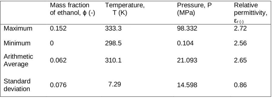
Table 2: Statistics of the input and output variables (validation data)

Mass fraction of ethanol, (-)

Temperature, T (K)

Pressure, P (MPa)

Relative permittivity,

r (-)

Maximum 0.152 333.3 98.332 2.72

Minimum 0 298.5 0.104 2.56

Arithmetic

Average 0.062 310.1 21.093 2.65

Standard

deviation 0.076 7.29 14.598 0.86

2.3 Performance Assessment for ANN Models

The performances of different ANN configurations were evaluated with different statistical

models, using the approach of Abidoye and Das (2014b). These statistical models are

expressed below:

A. Sum Squared Error (SSE)

This describes the total deviation of the predicted values (Scal) from the target values (Sobs):









 N

i

ca l obs S S SSE

1

2

(1)

Where N = Total number of data points predicted, Sobs= observed or target value of r, and

B. Average Absolute Relative Error (AARE)

This is the average of the relative errors in the prediction of a particular variable and it is

expressed as a percentage. Lower values of AARE indicate better model performance. It

can be computed as follows:

100 1 1      N n _obs obs cal S S S N AARE (2)

C. Nash-Sutcliffe Efficiency Coefficient (NS)

The Nash-Sutcliffe efficiency coefficient is used to describe the accuracy of model outputs in

relation to observed data. A value of NS equal to 1 depicts a perfect match between

observed data and outputs. Therefore, the closer the model efficiency is to unity, the more

accurate the model. NS is computed as follows:









Where S_obs = average of the observed output.

D. Mean squared error (MSE)

Mean squared error measures the average of the squares of the errors between the

observed value (Sobs) and the predicted or estimated value (Scal). For number of data points

or cases, N, MSE can be obtained by averaging the SSE as,





 





N

n obs ca l

S S N MSE 1 2 1 (4)

Note: In this work, ‘n’ is the sequential data count and ‘i’ is the sequential neuron count

2.4 Procedure for Developing ANN-based Equation from Weights and Biases

As said earlier, mixtures of CO2 with other compounds are often employed in industry to

achieve better results in extraction processes. Also, impurities are often encountered in CO2

stream obtained from the different emission sources, from which CO2 is captured for

geological storage site, poses unforeseen dangers to the pipeline and even storage aquifers.

Therefore, developing a simple equation to detect or quantify the amount of these impurities

through the determination of different r for pure CO2 and its mixtures, under different

conditions, will be of immense benefits in research and industry. Steps followed in this work

can be employed to achieve this objective.

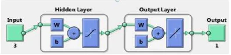
Figure 1: Typical network arrangement in a single-hidden layer ANN model (Mathworks Inc.,

USA). In the figure there are 3 input variables and 1 output

Figure 1 shows the typical arrangement in a single-hidden layer configuration of ANN model.

The figure shows that the model has three input variables (e.g., , T and P) and one output

variable (e.g., r). ‘w’ and ‘b’ represent the weights and biases, respectively. Their values are

randomly assigned by the network. In the hidden layers, there are neurons, whose number

depends on the choice or design of the user. In this work, different numbers of neurons are

tested in the configurations of both single and double-hidden layers. In the case of a double

hidden layer, two hidden layers will be shown in Figure 1, instead of one. In the figure, the

transfer function associated with the hidden layer is called ‘Tansig’. It is shown with a curve

in the hidden layer. In the output layer, the associated transfer function is ‘Purelin’ and it is

shown as a straight line.

The procedure in developing ANN-based equation involves the extraction of necessary data

from the operational procedure of ANN. The steps include the following:

ANN begins operation with the normalization of the input data. The function used for the

normalization in our simulation is called mapminmax, which scales inputs and targets so that

they fall in the range 1 to -1, corresponding to the highest and lowest values, respectively.

The equation for mapminmax is shown in equation (5).

min min max min min max y ) X X ( ) x x ( * ) y y ( y    

 (5)

where ‘y’ is the normalised value of X, ‘ymax’ is 1, ‘ymin’ is -1, ‘X’ is the actual value of

parameter (independent variable) of interest, ‘Xmin’is the minimum value of the parameter of

interest, ‘Xmax’ is the maximum value of the parameter of interest.

Having defined the normalisation function (mapminmax), the first task was that each of the

input parameters in our work (i.e., , T and P) be expressed in normalised form, using

equation (5). The normalised values of , T and P are represented as



) (nor m

P , respectively. Their sequential counts in the data list are represented as:

n ) norm (  , n ) norm (

T , and

n ) norm (

P , respectively,

B. Weight assignments at the hidden layer

Following normalization of input variables, the assignments of weights and biases to the

normalised variables, were performed. In Figure 1, this process is indicated with ‘W’, ‘b’,

referring to weights (W) and biases (b) that were automatically generated by the network.

The relationship is linearly developed using the equation:

   





j

i li nor mn liT nor mn liP nor mn li n

i

l W W T W P b

E

1 ,, ( ) ,, ( ) ,, ( ) ,

,

,  * * * (6)

where ‘Wl,i, ’, ‘Wl,i,T’and ‘Wl.i,P’ refer to the weights assigned, respectively to the Mass fraction

of ethanol ( ), Temperature (T) and Pressure (P) in association with the particular neuron (i)

(i). n ) norm (  , n ) norm (

T , and

n ) norm (

P , are the nth values of normalised , T and P, respectively.

‘El,i,n’ refers to the nth sum of the weighted normalised variables, based on the weight

assignment in association with ith neuron at the particular hidden layer (l). ..j is the last count

of neuron in the network.

C. Transfer function at the hidden layer

Following Figure 1, the next step in developing the ANN-based model requires mathematical

operation on the last step, using Tansig transfer function. The function is mathematically

expressed as: 1 ) 2 exp( 1 ( 2 ) ( , , , , , ,   _{ }  n i l n i l n i l E F E

Tansig (7)

It must be noted that the description above was limited to the single-hidden layer model for

the sake of simplicity. In the case of the double-hidden layer, there will be two levels of

‘Tansig’ transfer function and each one is to be treated, separately.

D. Weight assignments and Purelin transfer function at the output layer

Still following the schematic of Figure 1 (for single-hidden layer network), at the output layer,

it can be observed that the step following ‘Tansig’ transfer function is the assignment of

weights and biases, followed by the application of ‘Purelin’ transfer function. For this output

layer, the weights and biases were also generated by the network. They are then assigned

to the previous variable (Fl,i,n) as shown in equation (8), using ‘Purelin’ function:





j

i oi lin

o W F b

a  

1 , ,,

* (8)

Where ‘Wo,i’refers to the weight at the output layer (o) attributed to each neuron (i); ‘Fl.i,n’ is

the previously defined value of the Tansig-transformed variable, associated with the sum of

the nth normalised input variable at the last hidden layer (l); ‘bo’ is the bias at the output

layer. ‘ao’ is the normalised final output.

To get the actual value of the output, there is a need to denormalise the output obtained in

equation (8). At this step, the normalised output (an) was denormalised, using equation (5).

In the equation, the task is to get ‘X’, instead of ‘y’. Therefore, ‘X’ is made the subject of the

formula.

3. Results and Discussions

Dielectric property (relative permittivity) can be used to detect the presence of CO2 and/or its

mixtures or impurities. In this work, efforts are made to describe how ANN model can be

used to characterise the dielectric properties of pure and impure CO2. This section begins

with the presentation of results and discussions on the performances of different ANN model

configurations. This is followed by the section showing results from stepwise procedures

used in developing an ANN-based model for the prediction of the r for pure CO2 and its

mixture with ethanol. It was emphasized how the techniques can be adopted in other CO2

mixture/impurities. Finally, the results and discussions on the applications of the model to

some practical cases of interest are presented.

3.1 ANN Models

As stated earlier, different configurations of the ANN models were tested to effectively and

efficiently predict the relative permittivity ( r) of the pure CO2 and its mixtures/impurities. This

testing of different configurations is necessary to ensure that the most reliable ANN structure

is applied to learn the trends and relationships in the range of data used. The well-trained

ANN model, having the best performance criteria, can then be used to predict the r values

applicable to the cases and conditions of interest. Therefore, this subsection presents the

results of the training, validation and testing, as well as the performances of the different

The performances in training, validation and testing as well as the post-training regression

are shown in Figures 2 and 3 for the single-layer (ANN[3-6-1]) model. For this configuration,

the “3” in the notation refers to the total number of variables in the input (i.e., mass fraction of ethanol, pressure and temperature), the following “6” refers to the number of neurons, used

in the first layer (the only layer in the single-layer case), while the last “1” denotes the

number of parameter in the output (i.e., r). Figure 2 shows how the mean squared error

(MSE) decreases, during training, validation and testing, as the number of epoch increases.

This eventually culminates in the optimal performance during validation at 43rd _epoch,

having MSE value of 2.0x10-4_{, approximately.}

Figure 3: Post-Training Regression Analysis of ANN[3-6-1].

This behaviour shows that the network learns better, as the number of epoch increases.

The post-training regression analysis (Figure 3) shows the linear regression fit to the data

points, matching the predicted output to the actual target. W ith a correlation coefficient (c) of

0.999, it can be inferred that the ANN model has performed very well.

The performances of all models are depicted and compared below:

3.2 Performances of ANN models

Performance-evaluation models listed in subsection 2.3 are used to compare and judge the

performances of all ANN models trained in this work. Figures 4 to 7 show the performances

of these models.

For the sum squared error (SSE) criterion, Figure 4 shows the results. The figure shows that

as the number of neurons increases, the error decreases. For the single-layer model, the

reduction in error becomes very noticeable as the number of neurons is more than two. The

ANN [3-6-1]. The model has the SSE of approximately 0.2596. For the double-hidden layer

models, the SSE becomes very low when the neurons in the first and second hidden layers

are more than two, i.e., ANN [3-2-2-1]. For the double-hidden layer models, the SSE

(0.3877) is least with ANN [3-4-1-1]. By comparison, it can be readily concluded that the

ANN [3-6-1] shows the best performance, judging from SSE values.

Figure 4: Sum squared error (SSE) for all ANN models in the prediction of relative

permittivity ( r) for pure CO2 and CO2/ethanol mixture.

The other criterion used in assessing the performance was average absolute relative error

(AARE). The results are shown in Figure 5. The performance pattern in this case was

similar to that shown for SSE. However, in comparison, AARE is higher than SSE for all the

models. Like before, ANN [3-6-1] has the least error, with AARE of 0.9946. 0

1 2 3 4 5 6 7 8 9 10

S

u

m

s

q

u

ar

ed

e

rr

or

,

S

S

E

(

-)

Figure 5: Average absolute relative error (AARE) for all ANN models in the prediction of

relative permittivity ( r) for pure CO2 and CO2/ethanol mixture.

The Nash-Sutcliffe Efficiency Coefficient indicates the efficiency of the prediction made by

the models. Figure 6 shows that many of the models have high efficiency.

Figure 6: Nash-Sutcliffe efficiency coefficient for all ANN models in the prediction of relative

permittivity ( r) for pure CO2 and CO2/ethanol mixture.

Thus, the models have good reliability in the prediction of the relative permittivity for the pure

CO2 and its mixture. However, critical inspection of the figure shows that ANN[3-6-1] has

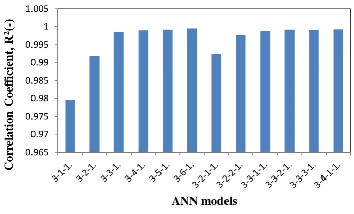
Similarly, the correlation coefficient (R2_{) was employed to judge the performances of the}

models. This is depicted in Figure 7. The closer the coefficient to 1, the better the

performance of the model. The Figure shows that the ANN [3-6-1] continues to exhibit the

best performance.

Figure 7: Correlation Coefficient (R2_{) for all ANN models in the prediction of relative}

permittivity ( r) for pure CO2 and CO2/ethanol mixture.

Based on the above criteria and results, it can be concluded that ANN [3-6-1] is the

best-performing configuration trained in this work. In comparison with publication from other

authors, the work of Nabavi-Pelesaraei et al. (2016) shows that their best network, having

nine neurons in each of the double hidden layers has the R2 _{value of 0.987. Even the RMSE}

value in their work is 0.054. Though, the complexity of the relationship may differ in their

work compared to this work, yet the values show our model has been sufficiently trained to

exhibit optimum performance in independent data prediction. As a result, this model

(ANN[3-6-1]) was used in developing the ANN-based equation for predicting r of pure and impure

CO2. The equation was also applied to independent cases of interests. These activities are

presented in the following subsections. 0.965

0.97 0.975 0.98 0.985 0.99 0.995 1 1.005

Cor

re

lat

ion

Coe

ff

icie

n

t,

R

2

(-)

3.3 ANN-based equation

As stated earlier, the objective of this work is to develop an ANN-based model, with which

the properties of the mixture and/or impurities of CO2 can be easily determined. The steps

in developing the model were already highlighted in section 2 of this work.

Following the lead from subsection 2.4, the equations of normalization for the independent

variables in the data used in the current work are,

1 343 . 9

norm 

 (9)

057 . 6 T 016668 .

0

T_norm  (10)

073 . 1 P 0211 . 0

P_norm  (11)

Where norm, Tnorm and Pnorm are the normalised values of , T and P, respectively (see

equation (5)).

Equation (6) expresses the assignments of weights and biases to the normalised variables

at the hidden layer of the network. The listed weights and biases in Table 3 are simplified

aggregates for each of the input variables, based on the six neurons in ANN [3-6-1]. The

arrangement in the table simplifies the mathematical operations occurring between

equations (6) and normalised input variables obtained from equation (5). Individual

normalised variables are already expressed in equations (9), (10) and (11). The weights and

biases indicated in the Table 3 are aggregates of the results obtained after the simplification.

Thus, ‘E’ value can be readily determined by multiplying the appropriate weights (in Table 3)

with actual values of the independent variables in the equation (6).

Still following the lead provided in the subsection 2.4 and Figure 1, the next step is the

‘Tansig’ transfer function for ‘E’ at the hidden layer. The expression for the transfer function

layer (see Figure 1 and equation (8)). Then, the resulting expression was denormalized, as

described in the subsection 2.4

The final expression for r after denormalization is shown in equation (12),

3324 . 4 F 1379 . 1 F 2223 . 0 F 3926 . 1 F 1234 . 0 F 0837 . 3 F 7234 .

2 1 2 3 4 5 6

r       

 (12)

where ‘Fl,i,n’ is given as ‘Fi’ for each of the six neurons in ANN [3-6-1], as defined in equation

(7). The subscripts 1…6 are for the six neurons in the singe hidden layer.

Therefore, interested readers only need to determine ‘E’ (using equation (6) and Table 3)

which is then used to determine ‘F’ using equation (7). The ‘F’ is then substituted into

equation (12) to determine the target relative permittivity ( r) of pure CO2 and/or its mixture

with ethanol.

Table 3: List of aggregate weights and biases for the normalised input variables used in

determining ‘El,i,n’ (see equation 6)* for ANN [3-6-1]**

Neurons(i…j) Weight, W1,i, Weight, W1,i,T Weight, W1,i,P Biases, b1,i

1 -2.56406 0.013246 -0.07972 -3.3363

2 -4.35511 0.011508 -0.00139 -2.18585

3 -1.97208 0.067772 -0.00354 -21.663

4 -3.7875 0.012443 -0.09534 -2.50458

5 26.76083 0.001232 0.008589 -1.78352

6 4.94227 -0.01721 0.072141 5.249718

*This is a single-hidden layer case. Thus, ‘1’ is indicated for ‘l’ in the symbols, i.e., W1,I,

** The weights and biases given have incorporated the coefficients and constants in the normalization

equations (9), (10) and (11). Thus, users only need to use the actual values of , T and P in the equation (6) together with weights (W) and Biases (b) in Table 3 to determine E.

3.4 Prediction of the

Having successfully established a new model in the previous sections of this work, based on

ANN [3-6-1], efforts are now made to use the model in predicting the behaviour of r for CO2

-ethanol mixture, under existing and new conditions. The first set of data used for the

predictions were earlier described in Table 2, which were independent experimental data

hypothetical conditions of temperature and pressure as well as ethanol concentration were

employed to further test the predictive ability of the model.

Figure 8 shows the effectiveness of equation (12) in predicting the new set of data at

different pressures. The validation data (see Table 2), at different pressures, were selected

for prediction, using the new equation. This selection of data was done to avoid overlapping

use of the data already used to train the model. From Figure 8, it is clear that the ANN model

captures the trend in the relative permittivity and pressure for wide range of pressure values,

with slight deviation occurring at peak pressure values, e.g., above 80 MPa.

Figure 8: Prediction of the experimental data, using equation (12).

Furthermore, equation (12) was used to test the case of the new set of data, where the mass

fraction of ethanol was 0.05. The result is shown in Figure 9, for the isothermal temperature

of 303.4 K. The figure shows that the new equation is effective in matching the new

experimental data. The r from the experiment and prediction overlaps over the range of the

pressure values. This shows that the model can perform effectively well in the face of a new

set of data. 0.8

1 1.2 1.4 1.6 1.8 2

0 20 40 60 80 100 120

R

e

la

ti

v

e

P

e

rm

it

ti

v

it

y

,

r

(-)

Pressure, P (MPa)

Selected Target Data (Actual Experiment)

Figure 9: Prediction of the new data (validation data described in Table 2), using model from

ANN [3-6-1]

Likewise, attempts were made at predicting the r for the same set of data (shown in Figure

9), but with the mass fraction of ethanol hypothetically increased by 100% i.e., from 0.05 to

0.1 (see Figure 10). It is clear from the result in Figure 10 that r increases with the rise in

mass fraction of ethanol.

Figure 10: Prediction of the change in r for increased from 0.05 to 0.1 using equation (12)

(ANN [3-6-1])

A similar trend was found using a new set of data, with increase of the mass fraction from

0.152 to 0.2 with an isothermal condition of 313.1K. The result of this is shown in Figure 11. 1.7 1.75 1.8 1.85 1.9 1.95 2

0 5 10 15 20 25

R e la ti v e P e rm it ti v it y , r (-)

Pressure, P (Mpa)

303.4K and =0.05

Experimental r

ANN 3-6-1 0 0.5 1 1.5 2 2.5 3

0 5 10 15 20 25

R e la ti v e P e rm it ti v it y , r (-)

Pressure, P (Mpa)

303.4K

ANN[3-6-1])

As before, r increases with mass fraction of ethanol. Thus, it can be concluded, that the

presence of ethanol increases the r of its mixture with CO2. This is similar to the conclusion

of Eltringham (2011). The author stated that relative permittivity increases with increasing

mass fraction of ethanol in the mixture.

Figure 11: Prediction of the change in r for increased from 0.152 to 0.2, using equation

(12) (ANN [3-6-1])

3.5 Effects of Change in Pressure and T

emperature on

Aside from predicting change in the mass fraction of ethanol in CO2, it is also interesting to

know the behaviour of r under changing conditions of pressure and temperature. Thus,

efforts were made at testing the performance of the model in predicting r at different

temperatures and pressures, using equation (12). The predicted results, shown in Figure 12,

show that the r increases with pressure for the same mass fraction of ethanol in the

mixture. In fact, it can be inferred that r increases linearly with the rise in pressure. This

result is similar to the findings of Abidoye and Das (2014a) as well as Mitchel and Mitchel

(1933). Mitchels and Mitchels (1933), in their classical work on the permittivity of CO2,

demonstrate how the permittivity of CO2 increases with pressure. Furthermore, Figure 13

shows that the r for the mixture decreases with increasing temperature. This is a reverse

trend to that of pressure effect on r. This conclusion has also been drawn by Eltringham

0 0.5 1 1.5 2 2.5 3 3.5

0 10 20 30 40

R

e

la

ti

v

e

P

e

rm

it

ti

v

it

y

,

r

(-)

Pressure, P (MPa)

313.1K

Experimental r)

(2011). The author concluded that under the conditions of isothermal pressure dependence,

r is always positive, while under the isobaric temperature dependence, it is always

negative.

Therefore the model developed in this work can serve well in the determination of impurities

in CO2, while the procedure can be extended to other popular mixtures of CO2 as well as

other gases. The results show that while monitoring CO2 behaviour in physical processes,

the model and/or method described in this work, can be used to determine or predict how

its dielectric property or that of its mixture will behave under different conditions.

Figure 12: Behaviour of r for CO2-ethanol mixture at different pressures: 10, 11, 15 and

20MPa. 1.65

1.7 1.75 1.8 1.85 1.9 1.95 2

10 11 15 20

R

e

la

ti

v

e

P

e

rm

it

ti

v

it

y

,

r

(-)

Pressure, P (MPa)

Figure 13: Behaviour of r for CO2-ethanol mixture at different temperatures: 333.2K,

366.52K, 370K and 390K

From the above work, it can be seen that the newly-developed ANN-based model is highly

effective under different conditions for the original and new sets of data. Therefore, the

model presented here is effective in predicting the r for CO2-ethanol mixture, while the

technique adopted in this work is also effective in determining the impurity content of CO2.

4. Conclusion

The application of Artificial Neural Network (ANN) for the prediction of the dielectric

properties of the mixture or impurities in CO2 has been elaborately demonstrated. By feeding

data of relative permittivity ( r) for pure and impure CO2 to the network, ANN was effectively

trained to recognise and predict CO2 property under different conditions.

Statistical analyses of the different ANN configurations showed that ANN model [3-6-1]

outperformed the others. From the best-performing ANN structure, this work further

extracted a single mathematical equation that can be employed in the prediction of the

relative permittivity ( r) for pure CO2 and CO2-ethanol mixtures, even without access to ANN

software. Using this ANN-based mathematical model, predictions of the relative permittivity 0

0.5 1 1.5 2 2.5 3

333.2 366.52 370 390

R

e

la

ti

v

e

P

e

rm

it

ti

v

it

y

,

r

(-)

Temperature (K)

( r) for pure CO2 and CO2-ethanol mixture were performed, under different temperature and

pressure and at different ethanol concentrations.

Under similar conditions, the output of the model provided good matches with original

experimental r. W ith an increase in ethanol concentration, the model correctly predicted the

rise in r for the mixture. It was also shown that the r rises with increase in pressure but

decreases with rise in temperature.

The work showed the reliability and applicability of the ANN in characterizing and predicting

the dielectric property of pure CO2 and its mixture and/or impurities. The model developed in

the work gives universal access to users, while the technique demonstrated offers insights

and a clear guide for researchers, who are interested in similar activities.

References

Abidoye, L.K., Bello, A.A., 2017. Simple dielectric mixing model in the monitoring of CO2

leakage from geological storage aquifer. Accept. Geophys. J. Int. 208 (3), 1787e1795.

https://doi.org/10.1093/gji/ggw495.

Abidoye, L.K., Das, D.B., Khudaida, K., 2015. Geological carbon sequestration in the context

of two-phase flow in porous media: a review. J. Crit. Rev. Environ. Sci. Technol. 45 (11),

1105e1147. https://doi.org/10.1080/10643389.2014.924184.

Abidoye, L.K., Das, D.B., 2015. Geoelectrical characterization of carbonate and silicate

porous media in the presence of supercritical CO2-water flow. Geophys. J. Int. 203 (1),

79e91. https://doi.org/10.1093/gji/ggv283.

Abidoye, L.K., Das, D.B., 2014a. pH, geoelectrical and membrane flux parameters for the

monitoring of water-saturated silicate and carbonate porous media contaminated by CO2.

Abidoye, L.K., Das, D.B., 2014b. Artificial neural network (ANN) modelling of scale

dependent dynamic capillary pressure effects in two-phase flow in porous media. J.

Hydroinformatics 17 (3), 446e461. https://doi.org/10.2166/hydro.2014.079

Astray, G., Iglesias-Otero, M.A., Morales, J., Mejuto, J.C., 2012. Relative permittivity of

carbon dioxide þ ethanol mixtures prediction by means of artificial neural networks. Mediterr.

J. Chem. 2 (1), 388e400.

Bielinski, A., Kopp, A., Schütt, H., Class, H., 2008. Monitoring of CO2 plumes during storage

in geological formations using temperature signals: numerical investigation. Int. J. Greenh.

Gas Control 2 (3), 319e328.

Boxberg, M.S., Prevost, J.H., Tromp, J., 2015. Wave propagation in porous media saturated

with two fluids. Is it feasible to detect leakage of a CO2 storage site using seismic waves?

Transp. Porous Media 107, 49e63. https://doi.org/10.1007/s1142-014-0424-2 .

Chadwick, A., Arts, R., Bernstone, C., May, F., 2008. Best Practice for the Storage of CO2 in

Saline Aquifers-Observations and Guidelines from the SACS and CO2STORE Projects.

Das, D.B., Gill, B.S., Abidoye, L.K., Khudaida, K.J., 2014. A numerical study of dynamic

capillary pressure effect for supercritical carbon dioxide-water flow in porous domain. AIChE

J. 60 (12), 4266e4278. https://doi.org/10.1002/aic.14577 .

Dethlefsen, F., K€ober, R., Sch€afer, D., Hagrey, S.A.A., Hornbruch, Gformation water

leakages into near-surface aquifers. Energy Procedia 37,4886e4893.

Eltringham, W., 2011. Relative permittivity measurements of carbon dioxide þ ethanol

mixtures. J. Chem. Eng. Data 56, 3363e3366.

Hanspal, N.S., Allison, B.A., Deka, L., Das, D.B., 2013. Artificial neural network (ANN)

modeling of dynamic effects on two-phase flow in homogenous porous media. J.

Keller, G.V., 1966. Section 26: electrical properties of rocks and minerals. Geol. Soc. Am.

Memoirs 97, 553e577.

Khashei, M., Bijari, M., 2014. Fuzzy artificial neural network (p, d, q) model for 600

incomplete financial time series forecasting. J. Intell. Fuzzy Syst. 26 (2), 831e845.

https://doi.org/10.3233/IFS-130775 .

Lamert, H., Geistlinger, H., W erban, U., Schütze, C., Peter, A., Hornbruch, G., Schulz, A.,

Pohlert, M., Kalia, S., Beyer, M., 2012. Feasibility of geoelectrical monitoring and multiphase

modeling for process understanding of gaseous CO2 injection into a shallow aquifer.

Environ. Earth Sci. 67 (2), 447e462 .

Lawan, S.M., Abidin, W.A.W.Z., Masri, T., Chai, W.Y., Baharun, A., 2017. W ind power

generation via ground wind station and topographical feedforward neural network (T-FFNN)

model for small-scale applications. J. Clean. Prod. 143,1246e1259 .

Little, M.G., Jackson, R.G., 2010. Potential impacts of leakage from deep CO2

geosequestration on overlying freshwater aquifers. Environ. Sci. Technol. 44, 9225e9232.

Mahmood, A., W arsi, M.F., Ashiq, M.N., Sher, M., 2012. Improvements in electrical and

dielectric properties of substituted multiferroic LaMnO3 based nanostructures synthesized by

co-precipitation method. Mater. Res. Bull. 47 (12), 4197e4202.

Marquardt, D.W., 1963. An algorithm for least-squares estimation of nonlinear parameters. J.

Soc. Ind. Appl. Math. 11 (2), 431e441.

Mathieson, A.,Wright, I., Roberts, D., Ringrose, P., 2009. Satellite imaging to monitor CO2

movement at Krechba, Algeria. Energy Procedia 1, 2201e2209.

https://doi.org/10.1016/j.egypro.2009.01.286 ,

Michels, A., Michels, C., 1933. The Influence of Pressure on the Dielectric Constant of

the Van der W aals Fund. In: Philosophical Transactions of the Royal Society of London.

Series A, Containing Papers of a Mathematical or Physical

Characteroyaloniesingersematical, Vol. 231, pp. 409e434.

Nabavi-Pelesaraei, A., Rafiee, S., Hosseinzadeh-Bandbafha, H., Shamshirband, S., 2016.

Modelling energy consumption and greenhouse gas emissions for kiwifruit production using

artificial neural networks. J. Clean. Prod. 133, 924e931.

Plug, W.-J., Bruining, J., 2007. Capillary pressure for the sandeCO2ewater system nder

various pressure conditions. Application to CO2 sequestration. Advances Water Resour. 30

(11), 2339e2353.

Qaderi, F., Babanezhad, E., 2017. Prediction of the groundwater remediation costs for

drinking use based on quality of water resource, using artificial neural network. J. Clean.

Prod. 161, 840e849.

Rabiu, K.O., Abidoye, L.K., Das, D.B., 2017. Geo-electrical characterisation for CO2

sequestration in porous media. Environ. Process. https://doi.org/10.1007/s40710-017-0222-2

Sharifi, A., Mohebbi, A., 2012. Introducing a new formula based on an artificial neural

network for prediction of droplet size in venturi scrubbers. Braz. J. Chem. Eng. 29 (03),

549e558.

Schwartz, M., 2014. Modelling leakage and groundwater pollution in a hypothetical CO2

sequestration project. Int. J. Greenh. Gas Control 23, 72e85.

Solymar, L., W alsh, D., Syms, R.R.A., 2014. Electrical Properties of Materials. Oxford

University Press.

Tokunaga, T.K., W an, J., Jung, J.-W., Kim, T.W., Kim, Y., Deng, W., 2013. Capillary

P c (Sw) controller/meter measurements, and capillary scaling predictions. W ater Resour.

Res. 49, 4566e4579. https://doi.org/10.1002/wrcr.20316 .

Wang, Z., 2015. Effects of Impurities on CO2 Geological Storage. M.Sc thesis, Submitted to

Faculty of Graduate and Postdoctoral Studies. University of Ottawa.