Predict Network, Application Performance Using Machine Learning and Predictive Analytics

Theses

5-2-2019

Predict Network, Application Performance Using

Machine Learning and Predictive Analytics

Mohamed Elmasry

[email protected]

Follow this and additional works at:https://scholarworks.rit.edu/theses

This Thesis is brought to you for free and open access by RIT Scholar Works. It has been accepted for inclusion in Theses by an authorized administrator of RIT Scholar Works. For more information, please [email protected].

Recommended Citation

Machine Learning and Predictive Analytics

Under Supervision of:

Prof Joseph Nygate, PhD

Submitted By:

Mohamed Elmasry

Thesis submitted in partial fulfillment of requirements of Degree of Master of Science in

Telecommunication Engineering Technology

Department of Electrical, Computer & Telecom Engineering Technology

College of Engineering Technology

Rochester Institute of Technology

Rochester, NY 14623

1 | P a g e

Committee Approval

Joseph Nygate, Ph.D. Date

Associate Professor, Thesis advisor

William P. Johnson, J.D. Date

Graduate Program Director, MS Telecommunications Engineering Technology Program

Mark Indelicato Date

2 | P a g e

Acknowledgments

I would like to express my sincere gratitude to my supervisor Dr. Joseph Nygate, who has

guided me through my coursework then later in my thesis. His valuable advice helped me in

overcoming several obstacles, which was standing in my way to complete my thesis work.

During the past year, I received many constructive feedbacks which assisted me in planning and

carrying out the research work. In addition, his insightful thoughts helped me to set up the

environment in a timely manner. Secondly, I am grateful to Mr. Mahesh Popli and Popli Design

Group for giving me permission to use the company network for collecting performance data

which was essential to my research work. Finally, I would like to thank my parents and friends

3 | P a g e

Table of Content

1. Abstract ... 6

2. Introduction ... 7

2.1 Literature Review ... 8

3. Architecture ... 11

3.1 Diagram ... 11

3.2 The Network Topology ... 12

3.3 Performance Metric Tools ... 13

3.3.1 Performance Monitor Tool ... 14

3.3.2 IPerf ... 16

3.3.3 PowerShell Scripts ... 17

3.3.4 Task Scheduler ... 20

3.3.5 Ku-Tools ... 20

4. Methodology ... 22

4.1 Collecting Data ... 22

4.2 Parsing the Data ... 27

4.3 Generating Graphs... 29

5. Results ... 33

5.1 Top Processes ... 33

5.2 Statistics Analysis ... 35

5.3 Decision Trees and Regression ... 40

6. Discussion ... 43

6.1 Limitation ... 45

6.2 Recommendation ... 45

7. Summary and Conclusion ... 46

4 | P a g e

Table of Figure

Figure 1: Architecture Diagram ... 11

Figure 2: Network Topology ... 12

Figure 3: Performance metric per extraction point ... 13

Figure 4: Performance Monitor Tool ... 15

Figure 5: Data Collector Set ... 15

Figure 6: Performance Monitor Output File ... 16

Figure 7: PowerShell Version ... 18

Figure 8: Ping Script ... 18

Figure 9: Top Process ... 19

Figure 10: IPerf Script ... 19

Figure 11: Task Scheduler ... 20

Figure 12: KU-Tools ... 21

Figure 13: Performance Monitor Scheduled Task ... 23

Figure 14: Task Trigger ... 24

Figure 15: Task Scheduler Action ... 25

Figure 16: Scheduled Task... 25

Figure 17: Ping Script Output ... 26

Figure 18: Top Processes Output ... 26

Figure 19: IPerf Script Output ... 27

Figure 20: Python Correlation Coefficient Code ... 28

Figure 21: Statistical Analysis describe method ... 29

Figure 22: Top Processes Python Code ... 29

Figure 23: Most Frequent Processes ... 30

Figure 24: Data Analysis Visualization ... 30

Figure 25: Decision Tree Python Code ... 31

Figure 26: Decision Tree Graph ... 32

Figure 27: Total CPU Time per Process ... 35

Figure 28: Measuring Decision Learning Model Accuracy ... 40

Figure 29: Decision Tree with seven Performance metrics ... 41

Figure 30: Decision Tree Rules ... 41

5 | P a g e

Tables of Tables

Table 1: Database Table... 12

Table 2: Network and Application Performance Metrics Per Tool ... 13

Table 3: Metrics Definition Table... 14

Table 4: IPerf Command Line Option ... 17

Table 5: Performance Monitor Output ... 23

Table 6: incorrect calculation for CPU Time Usage ... 34

Table 7: Correction calculation for CPU Time usage ... 34

Table 8: describe method output ... 36

Table 9: Resource Consumption summation ... 37

Table 10: Pearson Correlation Coefficient ... 38

Table 11: Spearman Correlation Coefficient ... 39

6 | P a g e

1.

Abstract

In this thesis, a study is performed to find the effect of applications on resource consumption

in computer networks and how to make use of available technologies such as predictive analytics,

machine learning and business intelligence to predict if an application can degrade the network

performance or consume computer system resources. In recent years, having a healthy computer

system and the network is essential for continuity of business. The study focusses on analyzing the

performance metrics collected from real networks using scripts and available programs created

specifically for monitoring applications and network in real-time.

This work has significant importance because monitoring real-time performance doesn’t give

accurate or concise information about the reasons behind any degradation in network or application

performance. On the other hand, analyzing those performance metrics over a certain period and

find a correlation between metrics and applications gives much more relevant information about

the root cause of problems.

The findings proved that there is a correlation between certain performance metrics, besides

correlation found between metrics and applications which conclude the study objectives. The

benefits of this study could be seen in analyzing complex networks where there is uncertainty in

7 | P a g e

2.

Introduction

Nowadays, Computer Networks are more complex than before, the number of applications

that runs on Clients/Servers increasing leading to a resources management problem. The IT

professionals tasked with maintaining the computer network facing serious challenges in

determining which applications consume computer resources or degrade network performance.

Analyze the performance metrics collected from Clients/Servers using traditional methods is not

enough anymore to make a correct decision whether an application consumes computer and

network resources. The improvement of the network performance is not an easy task, even with

network bandwidth upgrade might not be an optimal solution to solve the problem of high

network utilization.

In this thesis will make use of machine learning and business intelligence and data analytics

to compare and show the benefits of using those techniques in analyzing network performance

metrics. Through collecting performance metrics from a real computer network. A constructed

database combine performance metrics will be further analyzed to find pattern and correlation to

give a better understanding of the application and network performance. The database will be

used to applying machine learning algorithms to predict future performance under certain

conditions. The implementation of those techniques in the future will cut the cost of running a

network and reduce investigation time whenever a problem occurs and make IT professional life

8 | P a g e

2.1 Literature Review

The predictive data analytics and machine learning evolution changed the world. The

applications are endless to apply those techniques to various aspects of life. Computer

networking can utilize predictive analytics and machine learning to monitor network

performance and further predict its performance [1]. The predictive analysis utilizes the

data-mining tools to make a prediction and provide a recommendation based on historical data [2].

The predictive analytics models can perform the statistical and analytics analysis on

diverse types of data. The data collected require preprocessing before applying predictive

analysis methods such as machine learning algorithms. The raw data is processed and

transformed into a format which is suitable for the future operation machine learning analysis or

business intelligence techniques.

The processed data used as input to the machine learning models to produce the required

prediction. The raw data is obtained by using data mining techniques. Data Mining is the

extraction of obscure or hidden predictive information next searching for a pattern using

techniques of statistical and pattern recognition such as decision trees and neural networks [2].

The data is divided into predictors and variables that are used to create a predictive model. The

study performed by using data mining to extract and find a hidden pattern from data collected in

a real computer network.

Machine learning algorithms such as decision trees are used to perform analysis on

network performance metrics after being divided into predictors and response variables [2].

Moreover, the data are analyzed using statistical techniques on the same network performance

metrics to compare the results of both techniques. The predictive analytics combines several

9 | P a g e

By using this approach, we combine several techniques stretched from statistics to

machine learning and data mining [3]. The data forecasting carried out by knowing the entire

elements of the decisions and using the decision models to find the relationship between those

elements [2]. The development of machine learning algorithms makes it easy to be used in

networking domain [1].

Machine learning algorithms can tackle problems in networking domains, create

unlimited potentials and unforeseen benefits in the next few decades. Classification and

prediction in machine learning can solve networking problems in network performance and

security. Those problems were very hard to deal with because of the complexity of networks.

The application of a machine learning in a typical network problem go through steps. The

first step identifying the problem type that requires attention (prediction, regression or decision

making). The second step collects unbiased data from network and applications that comprise

application performance logs, network metrics, etc. The third step is performed analysis on the

data being collected from preprocessing to feature extraction [1]. The fourth step is model

construction that’s basically a learning model or algorithm require training using data [1]. Step

five is model validation which involves accuracy testing and verifies if the model is overfitting.

The last step called deployment and inference because the implementation phase requires

10 | P a g e

Learning depends on data availability and accuracy. The real-time responses from a

learning model require having a huge amount of historical data and a very complex learning

model. In the study, the learning model doesn’t provide real-time responses, but it can analyze

historical data when it is presented [1]. The learning model able to predict the applications which

consume computer resources such as CPU utilization. The goal is to improve the network and

11 | P a g e

3.

Architecture

The Architecture shows an overview of the entire experiment and the testbed environment

created to prove the thesis statement.

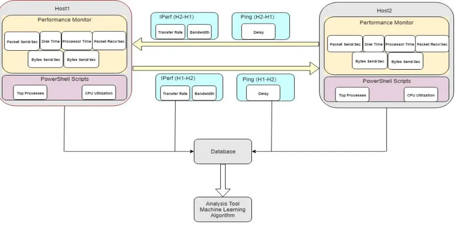
3.1 Diagram

The following diagram represents the network topology and name of tools used to collect

the data from client/server as well as communication links. The diagram illustrates the flow of

data between client/server and PowerShell scripts created to retrieve application metrics and

CPU utilization from client/server. In addition, it shows the commands run on client/server that

is used to test communication links between them. Every monitoring tool, PowerShell script, and

command runs on the client/server produce an output file (raw data). Those files require

preprocessing to transform data into a suitable format to apply data analytics techniques and

machine learning algorithm.

12 | P a g e

3.2 The Network Topology

The below figure represents the network topology and shows how the two hosts are

connected and can reach each other.

• The network topology is a hub and spoke • Host1 located in the main office

• Host2 located in one of the remote branches

• Remote offices are connected through a VPN Tunnels or Leased Line connection.

Figure 2: Network Topology

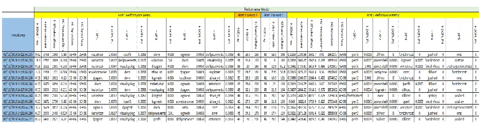
The following table represents the database that was created from processing the output

files from PowerShell scripts, Performance monitor, IPerf network testing tool and commands

run on Client/Server.

13 | P a g e

3.3 Performance Metric Tools

The network and application performance is measured through several performance

metrics such as Bandwidth, Throughput, Disk time, CPU Utilization, number of packets send/Recv

per sec, and number of bytes send/Recv per send.

The testbed used in the implementation has several tools to collect network and application

metrics. The metrics collected on both hosts and the communication links between two hosts.

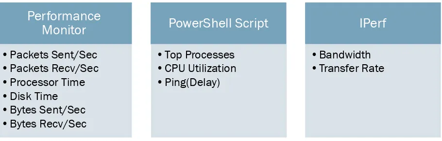
The below tables show the performance metrics categorized by the tool used:

Table 2: Network and Application Performance Metrics Per Tool

The below figure shows performance metrics categorized by the metric extraction point:

Performance

Monitor

•Packets Sent/Sec

•Packets Recv/Sec

•Processor Time

•Disk Time

•Bytes Sent/Sec

•Bytes Recv/Sec

PowerShell Script

•Top Processes

•CPU Utilization

•Ping(Delay)

IPerf

•Bandwidth

•Transfer Rate

Figure 3: Performance metric per extraction point

Performance Metrics

Host Metrics

Packet

Sent/Sec Recv/SecPacket Disk Time Processor TIme UtilizationCPU ProcessesTop Sent/SecBytes Recv/secBytes

Communication Link Metrics

Delay

14 | P a g e

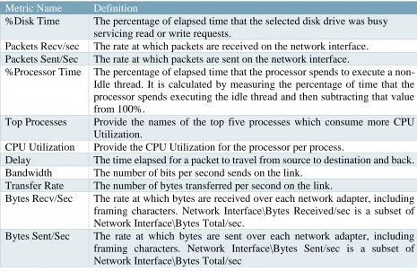
The table below shows network and application performance metrics definitions:

Table 3: Metrics Definition Table

Metric Name Definition

%Disk Time The percentage of elapsed time that the selected disk drive was busy servicing read or write requests.

Packets Recv/sec The rate at which packets are received on the network interface. Packets Sent/Sec The rate at which packets are sent on the network interface.

%Processor Time The percentage of elapsed time that the processor spends to execute a non-Idle thread. It is calculated by measuring the percentage of time that the processor spends executing the idle thread and then subtracting that value from 100%.

Top Processes Provide the names of the top five processes which consume more CPU Utilization.

CPU Utilization Provide the CPU Utilization for the processor per process.

Delay The time elapsed for a packet to travel from source to destination and back. Bandwidth The number of bits per second sends on the link.

Transfer Rate The number of bytes transferred per second on the link.

Bytes Recv/Sec The rate at which bytes are received over each network adapter, including framing characters. Network Interface\Bytes Received/sec is a subset of Network Interface\Bytes Total/sec.

Bytes Sent/Sec The rate at which bytes are sent over each network adapter, including framing characters. Network Interface\Bytes Sent/sec is a subset of Network Interface\Bytes Total/sec

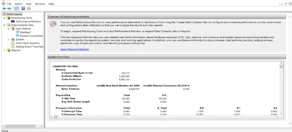
3.3.1 Performance Monitor Tool

Performance Monitor Tool used to view performance data in real-time or produce logs

files. Performance monitor tool is a built-in tool within Windows and doesn’t require any

installation. The requirement to obtain performance metric data is to configure a data collector

set. The output of the data collector is configured to produce a Comma Separated file that will be

used in further analysis. Creating a data collector set and configure it through adding specific

metrics require collecting. The study focuses on collecting metrics related to applications and

15 | P a g e

Figure 4: Performance Monitor Tool

Metrics added on data collector set

• Packets Recv/sec • Packets sent/sec • Bytes Recv/sec • Bytes Sent/sec • Processor Time • Disk Time

16 | P a g e

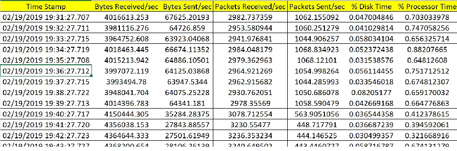
The below Figure show the output log file from Performance Monitor Tool:

Figure 6: Performance Monitor Output File

3.3.2 IPerf

It is a tool used to test network bandwidth and provide measurement [4], IPerf can

generate TCP/UDP traffic. IPerf uses a client/server model. It's compatible with several

platforms from Windows/Linux. IPerf has built-in features to customize the testing process and

dump the output into CSV files for further analysis. The IPerf support different protocols (TCP,

UDP, SCTP with IPv4 or IPV6). IPerf reports two important network performances metrics

(Transfer Rate, Bandwidth). IPerf version used on the testbed and the real environment is version

iperf-3.1.3. IPerf command can make use of any of the following programs to run its commands

17 | P a g e

The below table explains option features which can be used to customize the testing command:

Table 4: IPerf Command Line Option

Command Line Option Description

-p, --port n The server port for the server to listen on and the client to connect

to. This should be the same in both client and server. The default is

5201.

-i, --interval n Sets the interval time in seconds between periodic bandwidth, jitter,

and loss reports.

-V, --verbose Give a more detailed output.

--logfile Send output to a log file.

-s, --server Run IPerf in server mode (This will only allow one IPerf

connection at a time).

-c, --client host Run IPerf in client mode, connecting to an IPerf server running on

the host.

-t, --time n The time in seconds to transmit for.

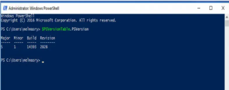
3.3.3 PowerShell Scripts

The PowerShell is a command-line task-based framework and scripting language from

Microsoft. For any System Administrator, it is a powerful tool that can be used to perform

different kinds of operation on any supported Windows platform, macOS and Linux. It used to

18 | P a g e

Figure 8: Ping Script

version 6 is independent of Windows, free and open source [5]. The PowerShell version utilized

in this research is version 5.1

Figure 7: PowerShell Version

The PowerShell is used in this research to develop scripts that automate the extraction of

network and application performance metrics from clients and servers running Windows

Platform. The developed script used to automate the running of IPerf network testing tool, collect

top processes which are utilizing CPU and ping command to test the delay on the network

between server and client.

The below figure shows the Ping script:

Test-Connection 10.5.1.229 -delay 60 -count 720 | Format-list @{n='TimeStamp';e={Get-Date}},__SERVER, Address,IPV4Address,ResponseTime | out-file

19 | P a g e

Figure 9: Top Process

The below figure shows Top-Processes script:

The below figure shows the IPerf script:

Figure 10: IPerf Script

function TopProcess { Param ( [Parameter(Position=1)] [Alias("l")] [int]$TotalList=5, [Parameter(Position=2)] [Alias("r")] [int]$Invertal=60 ) Begin {} Process { While ($true) {

$CounterSamples = Get-Counter '\Process(*)\ID Process','\Process(*)\% Processor Time','\Process(*)\Working Set' | Select-Object -Expand CounterSamples

Clear-Host

$CounterSamples | Group-Object { Split-Path $_.Path } | Where-Object {$_.Group[1].InstanceName -notmatch "^Idle|_Total|System$"} | Sort-Object -Property {$_.Group[1].CookedValue} -Descending | Select-Object -First $TotalList | Format-Table

@{n='TimeStamp';e={Get-Date}},@{Name="ProcessId";Expression={$_.Group[0].CookedValue}},@{Name="ProcessorUsage";Expression ={[System.Math]::Round($_.Group[1].CookedValue/100/$env:NUMBER_OF_PROCESSORS,4)}},@{Name="Pr ocessName";Expression={$_.Group[1].InstanceName}},@{Name="WorkingSet";Expression={[System.Math]::Ro und($_.Group[2].CookedValue/1MB,4)}}

Sleep -Seconds $Invertal }

} End {} }

TopProcess | Out-File C:\Users\melmasry\Desktop\ThesisWork\Server-Task.txt -Append

cd c:/

cd iperf-3.1.3-win64

20 | P a g e

3.3.4 Task Scheduler

The task scheduler enables the Windows users to automate tasks and run scripts on specific

times and run programs or even sending emails. There are several features to utilize and allow

more control parameters to be adjusted in any scheduled running task. The task scheduler is built

in several Windows platforms by default.

Figure 11: Task Scheduler

The main components of task scheduler that were utilized in this research are:

• Task Action • Task Trigger • Repeating A Task

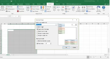
3.3.5 Ku-Tools

It is an add-on used with excel Microsoft, allow advanced functions and operations to be

implemented on excel, CSV files. The function that is used in this research called Transform

21 | P a g e

22 | P a g e

iperf.exe -c 10.5.1.229 -i 60 -t 900 -p 5021 -V --logfile client-iperf.csv

4.

Methodology

The experiment is carried out to find the effects of applications on resource consumption

in computer networks through extracting performance metrics. The data is analyzed using

machine learning and data analytics techniques, also finding any correlation exists between those

metrics. The performance metrics are extracted from the client as well as the server. The client is

accessing files on the server or using installed network applications.

The synchronization between tasks running in this experiment is the most important

factor to have accurate performance metrics which converted into a database. The performance

metrics are measured and extracted using installed independent software, built-in programs

within the Windows Operating Systems.

4.1 Collecting Data

The software used are Performance Monitor, Task Scheduler, PowerShell Scripts, and

IPerf network testing tool. IPerf is introduced into the experiment to test network bandwidth and

transfer rate. This aims at increasing the amount of the data exchanged between the client and the

server. The IPerf tool generates UDP or TCP traffic protocols. In this experiment, only a TCP

traffic is generated by IPerf tool. Windows PowerShell is used to run IPerf commands. A

PowerShell script is created and imported into Task Scheduler and configured to run at a specific

time. The performance metrics are collected every one-minute interval.

23 | P a g e

iperf.exe -c 10.3.1.8 -i 60 -t 900 -p 5021 -V --logfile server-iperf.csv

iperf.exe -s -p 5021

• Command used to initiate traffic from the server to the client (run on the server):

• Command used to allow the client and server to listen to port 5021(run on server and client):

The data collection tasks are required to run exactly at the same time across the client or

servers. The main reason behind this is to take a snapshot from performance metrics on both the

client and server at the same second in time.

The Performance Monitor has a component called schedule. This component is used after

data collector set created and performance metrics were added.

Figure 13: Performance Monitor Scheduled Task

Data collector set is configured to generate a CSV file that is preprocessed and later

analyzed. The below table shows the CSV output file from Performance Monitor.

24 | P a g e

Task Scheduler is used to schedule PowerShell Scripts to start at the exact time. Task

Trigger component is used to perform this operation.

Figure 14: Task Trigger

Task Scheduler component is used Task Action to import PowerShell script to run.

Argument Option is used to locate PowerShell Script

25 | P a g e

Task Scheduler is used to run three different PowerShell scripts scheduled to run at the

same time on both the client and server:

• Task 1: IPerf script

• Task 2: Ping command script • Task 3: Top Processes script

Figure 16: Scheduled Task

Each of the script used in task scheduler provides an output file. The output file is

text-based that requires preprocessing before converted into a database. The PowerShell scripts are

designed to provide output accompanied by a time stamp. This time stamp is used to align the

output of all PowerShell scripts, Performance Monitor and IPerf Script.

26 | P a g e

The below figures show the output of Ping Command PowerShell script, the PowerShell

script used in this experiment implemented another command is used as a replacement and provide

the same output called Test-Connection:

Figure 17: Ping Script Output

The below figure shows the output of Top Processes PowerShell script:

Figure 18: Top Processes Output

27 | P a g e

Figure 19: IPerf Script Output

4.2 Parsing the Data

The output from the PowerShell scripts is pure text files. Those files require processing to

extract the required data. Each text file is imported into Microsoft Excel and using KuTools

an add-in. The transform function among other advanced operations used to extract the

required performance metrics.

A database is constructed from the data extracted from PowerShell script output. The

database columns consist of two sides, one side represents the performance metrics of the

client and the other side the server. Each row in the database represents performance metrics

collected in the one-minute interval. Once the database is created, the analysis phase using

28 | P a g e

Figure 20: Python Correlation Coefficient Code

Python is a powerful programming language that can be used in many different fields to

solve real-world problems. Python has rich libraries that allow the programmers to perform

many actions without having to write long code. In the thesis work, Python programming

language along with a couple of libraries are utilized to analyze the data using machine

learning and data analytics. The Pandas library provides data manipulation and analysis tools.

The Numpy library provides high-level mathematical functions that can work on

multi-dimensional arrays. The scikit-learn library is a free machine learning library provides

classification, regression and clustering algorithms. It's used in this research work for

regression and decision trees. The matplotlib library is a powerful plotting library for Python

that can be incorporated with other libraries such as Pandas and Numpy.

The statistical analysis used to understand the nature of the data being analyzed. It’s a

component of data analytics and related to business intelligent [6]. It is applied to the

database using Python powerful libraries and mathematical functions to identify the trends

and find patterns in structured and semi-structured data. The database is analyzed to find the

correlation coefficient between application and network performance metric. The correlation

coefficient provides us with insights into the cause-effect relationship between performance

metrics. There are three correlation coefficient methods (Pearson, Kendall, Spearman).

Below figure shows an example python code used to calculate the Spearman correlation

coefficient:

import pandas as pd import numpy as np import math as m import statistics

FileServer = pd.read_csv('FileServerMetrics.csv')

29 | P a g e

import pandas as pd import numpy as np

import matplotlib.pyplot as plt %matplotlib inline

import seaborn as sns

Server = pd.read_csv('Server-2.csv')

pd.set_option('display.float_format', lambda x: '%.4f' % x) plt.rcParams["figure.figsize"] = (20,20)

plt.xlabel('occurance') plt.ylabel('process names')

Server.H2P1.value_counts().plot(kind='Barh')

Figure 22: Top Processes Python Code

The statistical analysis is continued to analyze the database by calculating standard

deviation, mean, count, percentile, minimum and maximum values for performance metrics.

The below figure shows the Python code as well as output obtained from using a Python

method called describe()

Figure 21: Statistical Analysis describe method

4.3 Generating Graphs

The database collected is analyzed further to find the trend in applications consumed the

resources in computer networks. One performance metric column “H1CPUP1” represent a top

process that used the CPU for the longest time per minute. Each value represents a process name

of an application installed on the client or server. The frequency of the process name in

“H1CPUP1” is investigated to determine the top applications that utilize the CPU.

The below figure shows the Python code used to find the most occurred top processes:

import pandas as pd import numpy as np import math as m import statistics

30 | P a g e

A graph generated as the output from the above Python code displays the most frequent

processes occurred as Top Process:

Figure 23: Most Frequent Processes

The seaborn library provides a toolset to draw graphs, the below graph represents pair plot

for performance metrics to show data analysis visualization of database and how much the data

are scattered.

31 | P a g e

The decision tree algorithm covers both regression and classification in machine learning,

this provides a wealth of information about performance metric database. The decision tree

provides a visual representation of the decisions and decision making through classification and

decision tree models. It is considered a data mining tool to enable finding a hidden pattern as

well as a prediction for future values. It revolves around asking the right questions to make better

decisions about which features are more important than others. In this research, the decision trees

illustrate which performance metrics have higher effects on the resource consumption and

performance prediction in the computer network. The performance metrics are divided into

groups predictor and target. The database is also divided into test and train sets into 20-80 or

10-90 split to increase precision.

The below figure shows the part of the code developed to create a decision tree and

visualized:

Figure 25: Decision Tree Python Code

Below decision tree figure shows prediction accuracy and classification for determining

future top processes that utilizing computer network resources.

X = df1.drop(columns=['H1P1']) Y = df1['H1P1']

x_train, x_test, y_train, y_test = train_test_split(X,Y,test_size=0.1) model = DecisionTreeClassifier(max_depth=4)

model.fit(x_train,y_train)

predications = model.predict(x_test) score = accuracy_score(y_test, predications) import graphviz

feature_names = list(df1.drop(['H1P1'], axis=1))

dot_data = tree.export_graphviz(model, out_file=None, filled=True, rounded=True, feature_names=feature_names,class_names=Y)

32 | P a g e

Figure 26: Decision Tree Graph

The learning model and the decision tree has been created then the training database is used

to train the model and test database used to verify the prediction of target top processes. The

33 | P a g e

5.

Results

The experiments started by setup a testing environment and scenarios to collect reliable

real-time data from a working network. The testing environment was carried out on a standalone

server. The built-in programs in windows operating system and developed PowerShell scripts

were tested to check their output if it matches what is required to run the experiment and obtain

accurate performance metrics values.

5.1 Top Processes

The first mission was choosing the significant performance metrics that have a high effect on

the application and network performance. The next step was finding a method to obtain values of

those performance metrics. A number of the performance metrics data were obtained using the

built-in programs while others were obtained through developing PowerShell scripts. The main

goal also is to automate this task.

The results obtained were not as expected in the beginning. For example, the CPU Time used

by a single application in one minute was required to determine which applications consume the

computer network resources. The challenge facing this task, the Windows Operating System

gives by default the accumulated time since the process started. A PowerShell script was

developed to perform this task calculates CPU Time used by the application in one minute. The

output was obtained as expected and required for the experiment success.

The two tables below show the difference in the result while trying to extract CPU Time used

34 | P a g e

Table 6: incorrect calculation for CPU Time Usage

Table 7: Correction calculation for CPU Time usage

The delay is an essential metric to characterize the network performance, it provides an

indication on the congestion of the network due to traffic utilized by application communicating

between client and server. The usual command used in most of operating systems is ping

command. The goal is to schedule sending a single ICMP ping packet every minute for a specific

period of time and the result of the delay should be accompanied by a time stamp of ping

initiation.

The first approach is to use the ping command, but it was ineffective in this experiment due

to lack of customization in output. Another approach was using a PowerShell script with a

command called test-connection, this command was appropriate and satisfy the need of this

35 | P a g e

5.2 Statistics Analysis

The data collection phase resulted in creating a performance database using the output from

multiple programs and scripts. The Analysis of this database resulted in an interesting finding.

The analysis included using data analytics techniques as well as applying machine learning

algorithms.

The database included five top processes who utilized the CPU Time in one minute. The first

column represents the number one in the list of top processes. The column was analyzed to

determine which applications are more frequent to appear in this column than others as well as

compare against the total time each process utilized the CPU Time. Using the matplotlib library

and describe a method to analyze the top process column.

36 | P a g e

Several applications appeared more than others but other applications who appeared less in

the Top Process column consumed more CPU Time. The result is logical and proves that it is not

about how frequent application usage CPU but for how long each application takes to complete a

certain task. An example, referring to the graph in figure 23 above, the most frequent Top

Processes is “logmein” while the second most frequent Top Processes is “IPerf3”. Examining the

graph in figure 27, we found that the second Top Processes used the CPU Time is svhost process

which contradicts that the second most frequent application appeared as the top process was

“IPerf3”.

Filtering the database to include only the values belong to the most frequent application

appeared as top process and analyze this part of the database. Using statistical methods to

calculate the min, max, mean, standard deviation and quartile provides insights about the data

distribution in each column. describe() method is used to provide this output.

Table 8: describe method output

mean std min 25% 50% 75% max SD/mean

H1DiskTime 0.6968 1.6632 0.0045 0.0323 0.0634 0.5982 15.4442 2.386911596

H1PacketsSent 1209.8453 1907.2108 1.2332 2.3332 36.9648 2296.6207 4817.5659 1.576408819

H1PacketsRecv 1163.8365 1834.906 1.8493 2.9665 49.6131 1822.2873 4619.0421 1.576601181

H1ProcessorTime 1.1159 0.7487 0.1303 0.9023 1.0226 1.1804 8.9249 0.670938256

H1BytesSent 1294659.1 1829841 122.32 5039.789 138766.58 2880897.7 6042295.7 1.413376683

H1BytesRecv 1406656.8 2336037.8 167.4 282.9439 57981.627 1856004.9 19384944 1.660702015

H1CPUP1 0.0038 0.0021 0.0005 0.002 0.0034 0.0049 0.0107 0.552631579

H1CPUP2 0.0008 0.0008 0 0.0005 0.0005 0.001 0.0078 1

H1CPUP3 0.0004 0.0006 0 0 0.0005 0.0005 0.0068 1.5

H1CPUP4 0.0003 0.0005 0 0 0 0.0005 0.0058 1.666666667

H1CPUP5 0.0001 0.0004 0 0 0 0 0.0058 4

H1Delay 34.0239 10.7934 28 30 31 33 166 0.317229947

37 | P a g e

The coefficient of variation (CV) is calculated by dividing the standard deviation over the

mean value. If the value is higher than 1 this means high standard deviation and data points are

tend not to be too close to each other. This is a measure for the spreading in the data points of

performance metrics. The performance metrics with a coefficient of variation larger than 1 refer

to having substantial changes through the data collection period. This allows the understanding

of the nature of the performance metrics and in the future improve the network and application

performance.

Each process consumes a certain amount of resources from CPU Time to how much delay

the network experience due to data exchanged between client and server. The following code

developed to combine the resource’s consumption by each process.

The table shows the output for each process accompanied by the total CPU time, Bandwidth

and delays the network experienced:

Table 9: Resource Consumption summation

H1P1 H1CPUP1 H1Delay H1BW acwebbrowser 0.144 798 534

csrss 0.0005 39 12.9 dattobackupagent 0.0029 68 10.5 dellpoaevents 0.3036 1156 746.24

dpagent 0.6462 2739 1789.33 dwm 0.6356 3279 5142.13 explorer 0.09 633 395.6 iastoricon 0.6639 2454 1567.4

iperf3 1.0323 7867 6377.7 iusb3mon 0.6186 2444 1657.17

logmein 2.8228 11482 8493.31 lsass 0.0159 209 156.9 niniteagent 0.2102 90 61.4

platform-agent-core

0.001 60 58.3

38 | P a g e

H1P1 H1CPUP1 H1Delay H1BW

platform- performance-plugin

0.0468 86 62.2

powershell 0.002 243 90.9 rocket.chat 0.0156 86 60.8 saazscheduler 0.0034 78 15.1 svchost 2.1914 1840 1048.26 visualsyslog 0.4127 1438 978

wmiprvse 0.093 455 242.3 wrsa 0.0699 305 213.8

The correlation coefficient provides insights if there is a mutual relationship or association

between quantities. In this research work, it is used to find if there are a cause and effect

relationship between performance metrics and measure the strength as well. The relationship can

be either positive or negative correlation and ranging between +1 and -1. It used to predict one

value from another present value.

Utilizing Python libraries and methods to calculate the correlation coefficient between the

performance metrics. There are several types of correlation coefficient that can be calculated for

the performance metrics. The below table shows the Pearson correlation coefficient between

several performance metrics:

Table 10: Pearson Correlation Coefficient

39 | P a g e

The Pearson correlation coefficient was used to calculate the correlation, but the results

showed it was not the best suitable coefficient type. Because it calculates a linear association

between continuous variables. The second correlation coefficient used is the Spearman

correlation coefficient, it is more appropriate for continuous and discrete data. The table below

shows the Spearman correlation coefficient for performance metrics:

Table 11: Spearman Correlation Coefficient

H1DiskTime H1PacketsSent H1PacketsRecv H1ProcessorTime H1BytesSent H1BytesRecv H1CPUP1 H1Delay H1BW H1TransferRate

H1DiskTime 1 -0.0945 -0.1498 0.2201 -0.0925 -0.1264 -0.0613 0.1219 -0.1159 -0.1152

H1PacketsSent -0.0945 1 0.9039 0.5941 0.991 0.9061 0.4324 -0.4963 0.4989 0.4971

H1PacketsRecv -0.1498 0.9039 1 0.6045 0.8852 0.8792 0.453 -0.4905 0.4738 0.4689

H1ProcessorTime 0.2201 0.5941 0.6045 1 0.5868 0.5373 0.5459 -0.282 0.331 0.3333

H1BytesSent -0.0925 0.991 0.8852 0.5868 1 0.8705 0.4355 -0.4772 0.5023 0.501

H1BytesRecv -0.1264 0.9061 0.8792 0.5373 0.8705 1 0.4028 -0.5273 0.4975 0.4974

H1CPUP1 -0.0613 0.4324 0.453 0.5459 0.4355 0.4028 1 -0.3558 0.4084 0.4039

H1Delay 0.1219 -0.4963 -0.4905 -0.282 -0.4772 -0.5273 -0.3558 1 -0.4179 -0.4137

H1BW -0.1159 0.4989 0.4738 0.331 0.5023 0.4975 0.4084 -0.4179 1 0.9978

H1TransferRate -0.1152 0.4971 0.4689 0.3333 0.501 0.4974 0.4039 -0.4137 0.9978 1

The Spearman correlation coefficient shows stronger association and relationship between

performance metrics because it looks at the monotonic relationship which is the variables

changes together but not with the constant rate. The third correlation coefficient utilized in this

research is the Kendall correlation coefficient. It is more suitable for a discrete variable.

Table 12:Kendall correlation coefficient

H1DiskTime H1PacketsSent H1PacketsRecv H1ProcessorTime H1BytesSent H1BytesRecv H1CPUP1 H1Delay H1BW H1TransferRate H1DiskTime 1.0000 -0.2402 -0.2076 0.4187 -0.1915 -0.2041 0.3613 0.2623 -0.1292 -0.1179

H1PacketsSent -0.2402 1.0000 0.6667 -0.2406 0.8688 0.5422 -0.1742 -0.3472 0.2858 0.2931

H1PacketsRecv -0.2076 0.6667 1.0000 -0.2278 0.5411 0.7769 -0.1735 -0.4033 0.2833 0.2870

H1ProcessorTime 0.4187 -0.2406 -0.2278 1.0000 -0.1840 -0.1829 0.5124 0.2377 -0.0608 -0.0763

H1BytesSent -0.1915 0.8688 0.5411 -0.1840 1.0000 0.4142 -0.1284 -0.2793 0.2759 0.2828

H1BytesRecv -0.2041 0.5422 0.7769 -0.1829 0.4142 1.0000 -0.1685 -0.3929 0.3220 0.3128

H1CPUP1 0.3613 -0.1742 -0.1735 0.5124 -0.1284 -0.1685 1.0000 0.2335 -0.0586 -0.0530

H1Delay 0.2623 -0.3472 -0.4033 0.2377 -0.2793 -0.3929 0.2335 1.0000 -0.2706 -0.2816

H1BW -0.1292 0.2858 0.2833 -0.0608 0.2759 0.3220 -0.0586 -0.2706 1.0000 0.9628

H1TransferRate -0.1179 0.2931 0.2870 -0.0763 0.2828 0.3128 -0.0530 -0.2816 0.9628

The Kendall correlation coefficient showed less association than the Spearman coefficient.

40 | P a g e

5.3 Decision Trees and Regression

The decision tree is basically a binary tree flowchart used to split the data into groups,

extremely helpful in classification and regression. The split is made according to certain

conditions or question aiming at categorizes the data with similar attributes to highlight hidden

information exist in data. In this research, decision trees are utilized to map and classify the

performance metrics to predictors and target. The decision tree algorithm used is a classification

and regression decision tree. Gini index value ranges from 0 (all target values belong to one

label) to a maximum value of 1(all target values are distributed equally). From Navigating the

decision tree, the applications that properly consume the resources in computer networks can be

predicted. The learning model accuracy was measured and provided accuracy between 70-80

percent. The below code shows the code and output for measuring the accuracy of the learning

model.

Figure 28: Measuring Decision Learning Model Accuracy

Dataset split into train and test, the highest accuracy achieved in splitting the dataset to 90%

train and 10% test. The results could be improved more with a larger dataset. Also, the maximum

41 | P a g e

The decision tree is taking the decision of splitting data based on rules, the figure 29 shows a

decision tree included the following performance metrics (H1BytesSent, H1BytesRecv,

H1DiskTime, H1ProcessorTime, H1PacketsSent, H1PacketsRecv, H1P1).

Figure 29: Decision Tree with seven Performance metrics

The below figure shows the rules created to generate the decision tree above:

Figure 30: Decision Tree Rules

Previously, the decision tree learning model was measured and it was expected to provide

accuracy from 70-80 %. The test dataset used as input to the learning model after using the train

dataset. A code was developed to compare between predicted output and the actual output of test

42 | P a g e

The output can be seen below, using a simple calculation to calculate the accuracy of the

output in percentage:

Figure 31: Decision Tree Accuracy Calculation

The calculation shows the accuracy is 77.95% that falls within the range of predicted value.

from pandas import DataFrame predict = model.predict(x_test)

43 | P a g e

6.

Discussion

The usage of machine learning and data analytics in computer networking has huge

potentials. In the thesis work, specific machine learning algorithm and data analytics techniques

were explored to find the benefits of applying those techniques and algorithm on a real-life

problem. In this case, the goal was to predict the application and network performance.

The work started by navigating and analyze a database constructed from collecting

performance metrics. The performance metrics were extracted from a real computer network.

The work started by using data analytics techniques. The statistical analysis put some lights on

hidden information unseen to the ordinary person. The nature of performance metrics become

easier to understand through the statistics and numbers.

Calculating the correlation coefficient has shown the cause and effect relationship between

performance metrics which is shown in high correlation discovered between processor time and

disk time among other correlation and association were discovered. As a result, the interpretation

of applications behavior is not impossible even in the complex computer networks. The

complexity of the network is not a concern or a factor anymore because the important is to

collect accurate metrics and data then analyze it.

The regression and classification of decision tree helped in predicting the future values of

resource consumption in the computer network. The CPU time consumed by application as well

as the amount of traffic send or received by edge nodes can be predicted with enough accuracy.

The measured accuracy was between 70-80 percent for the decision tree. The accuracy of the

44 | P a g e

In this study, a private company network was used to collect the performance metrics from

its clients and servers, in addition to, the communication links between branches. The data

analytics results were interesting. We were able to find the applications that consume most of the

resources at the company network. For example, two processes named logmein and svchost

consumed most of the CPU time.

We were able to calculate the proper correlation coefficient to discover the association

between performance metrics. The performance is affected by the amount of data exchanged

between client/server. A positive correlation was discovered between the number of packets

sent/recv per second and processor time. Consequently, the processor time increase as a response

to the increment number of packets exchanged between the clients/server.

The calculation of the standard deviation, mean and quartile explained the data point samples

taken from each performance metrics. The processor time had a coefficient of variation less than

one (0.67) indicating that the difference between processor time data point is minimal. On the

other hand, the coefficient of variation disk time was bigger than one (2.386) informing us that

the data point collected have a long margin.

We were able to create a decision tree using the metrics collected from the company network

and the target was predicting the application that consumes CPU time most of the time. The

model was trained using dataset then, using a test sample compromised from 127 samples. The

success rate reached 77.9% for this experiment.

The findings can help any IT professionals to analyze the application and network

performance and obtain information with acceptable accuracy on the application consumes the

45 | P a g e

6.1 Limitation

The experiment was performed on a standalone server. The goal was to isolate any failure

which can result in interrupting the business in case of using a real-life computer network. This

extended the time frame of establishing a working environment. The multiple simultaneous

actions and the synchronization between the task are essential factors in the success of the

experiment. The experiment requires having a huge database to obtain a good result.

Consequently, the data collection phase took a long time to prepare a dataset big to provide

reliable results.

6.2 Recommendation

The thesis work proved that there is a potential to take this work further and recommendation

to apply other data analytics techniques and machine learning algorithms. The work requires

more care when creating the database from performance metrics because of the sensitivity of

46 | P a g e

7.

Summary and Conclusion

The application and network performance are a major concern for the network

professional. The thesis addressed several concerns related to determining the applications that

may misuse the resources in the computer networks. The suggested techniques to address and

solve this problem relied on using high trended technologies machine learning and data analytics.

Both techniques have the reputation of solving many problems in a variety of field. The

work resulted in understanding more about the network and application performance metrics. In

addition, the nature of the metrics if they are categorical or continuous or discrete. Moreover, the

cause and effect relationship between performance metrics by calculating the correlation

coefficient. Furthermore, the decision trees helped in the prediction of application performance

through analyzing and classifying the performance metrics.

The performance metrics that are responsible for affecting or consuming the resources in

the computer network can be predicted with satisfactory accuracy ranging between 70-80%. The

decision tree graphs were able to show the classification of performance metrics and the changes

in values would affect the target performance metric.

The application of this work will cut cost and provide substantial benefits to IT

professionals and mid-large companies to optimize the network and application performance.

Nowadays, as the networks become more complex and applications requires much more

resources. The traditional approaches to deal with network and application performance is not

enough. The thesis work could be extended to provide more benefits through using other

47 | P a g e

8.

References

[1] Y. C. X. W. S. X. a. J. J. Mowei Wang, "Machine Learning for Networking: Workflow, Advances, and Opportunities," IEEE Network.

[2] N. Mishra and S. Silakari, "Predictive Analytics: A Survey, Trends, Applications,

opportunities & challenges," International Journal of Computer Science and Information Technologies, no. 0975-9646, 2012.

[3] K. Wakefield, "www.sas.com," [Online]. Available:

https://www.sas.com/en_gb/insights/articles/analytics/a-guide-to-predictive-analytics-and-machine-learning.html.

[4] C. Schroder, "wikipedia," [Online]. Available: https://en.wikipedia.org/wiki/Iperf.

[5] J. Aiello, C. Shawn, and S. Wheeler, "PowerShell Version 6," 26 08 2018. [Online]. Available:

https://docs.microsoft.com/en-us/powershell/scripting/overview?view=powershell-6.

[6] M. Rouse, "statistical analysis," [Online]. Available: https://whatis.techtarget.com/definition/statistical-analysis.

[7] R. Boutaba, M. A. Salahuddin, N. Limam, S. Ayoubi, N. Shahriar, F. Estrada-Solano and O. M. Caicedo, "A comprehensive survey on machine learning for networking: evolution, applications, and research opportunities," Journal of Internet Services and Applications,

2018.