Rochester Institute of Technology
RIT Scholar Works
Theses Thesis/Dissertation Collections
2-1-2012
Low power context adaptive variable length
encoder in H.264
Soumya Lingupanda
Follow this and additional works at:http://scholarworks.rit.edu/theses
Recommended Citation
Low Power Context Adaptive Variable length
Encoder in H.264
By
Soumya Lingupanda
A Thesis Submitted in Fulfillment of the Requirements for the Degree of Master of Science in Computer Engineering
Supervised by Professor Dr. Kenneth Hsu Department of Computer Engineering
Kate Gleason College of Engineering Rochester Institute of Technology
Rochester, NY
Approved By:
__________________________________________________________
Dr. Kenneth Hsu, Professor
Primary Advisor – R.I.T. Dept. of Computer Engineering
__________________________________________________________
Dr. Dhireesha Kudithipudi, Assistant Professor
Secondary Advisor – R.I.T. Dept. of Computer Engineering
__________________________________________________________
Dr. Amlan Ganguly, Assistant Professor
Secondary Advisor – R.I.T. Dept. of Computer Engineering
Abstract
The adoption of digital TV, DVD video and Internet streaming led to the development of
Video compression. H.264/AVC is the industry standard delivering highly efficient and
reliable video compression. In this Video compression standard, H.264/AVC one of the
technical developments adopted is the Context adaptive entropy coding schemes.
This thesis developed a complete VHDL behavioral model of a variable length encoder.
A synthesizable hardware description is then developed for components of the variable
length encoder using Synopsys tools. Many implementations were focused on density and
speed to reduce the hardware cost and improve quality but with higher power
consumption. Low power consumption of an IC leads to lower heat dissipation and
thereby reduces the need for bigger heat sinking devices. Reducing the need for heat
sinking devices can provide lot of advantages to the manufacturers in terms of cost and
size of the end product. Focus towards smaller area with higher power consumption may
not be appropriate for some end products that need thinner mechanical enclosures
because even if the design has smaller area it needs a bigger heat sink thereby making the
enclosures bigger. This thesis therefore aimed at low power consumption without
compromising much on the area. The designed architecture enables real-time processing
Table of Contents
1 Overview... 1
1.1 Video Coding Overview ... 1
1.2 HW/SW CAVLC Design... 4
2 Background Theory ... 5
2.1 Video Compression... 5
2.1.1 Encoder ... 7
2.1.2 Decoder ... 8
2.2 H.264... 10
2.2.1 Prediction Block... 11
2.2.2 Transform and Quantization block ... 16
2.2.3 Encoding ... 20
3 Context Adaptive Variable Length Coding (CAVLC)... 23
3.1 Coefficient token... 24
3.2 T1 sign ... 24
3.3 Level ... 24
3.4 Total zeros... 25
3.5 Run before... 25
4 CAVLC ARCHITECTURE ... 26
4.1 Zigzag Scan Block ... 27
4.2 Ngen block ... 28
4.3 Coeff_token block... 28
4.4 Total Zeros block ... 29
4.5 Level block... 30
4.6 Run before block... 31
4.7 Bitstream generator... 32
5 Simulation and Synthesis Results... 33
5.1 Zigzag Scan Block Simulation... 33
5.2 Ngen block Simulation ... 33
5.3 Coeff_token block Simulation ... 35
5.4 Total Zeros block Simulation... 35
5.5 Level block Simulation ... 37
5.6 Run before block Simulation ... 37
5.7 Bitstream generator block Simulation ... 38
5.8 Results... 43
6 Conclusion ... 45
List of Figures
Figure 1: H.264 Baseline Profile Encoder [1]... 4
Figure 2: Video Compression[1]... 6
Figure 3: Baseline Profile Decoder... 9
Figure 4: Encoder and Decoder ... 10
Figure 5: Macroblock... 12
Figure 6: 4x4 Intra Prediction Patterns (sub-block)... 14
Figure 7: 16x16 Intra Prediction Patterns[3]... 14
Figure 8: Tree Structured Macroblock Partitions ... 16
Figure 9: 16x16 Macroblock Block Ordering[5]... 21
Figure 10: Zig-Zag Scan Order... 22
Figure 11: Proposed CAVLC Architecture... 26
Figure 12: Zigzag simulation ... 34
Figure 13: Ngen simulation ... 34
Figure 14: Coefftoken simulation ... 34
Figure 15: Totalzeros simulation ... 34
Figure 16: Level simulation ... 35
Figure 17: Run before simulation ...36
Figure 18: Bitstream simulation... 37
Figure 19: CAVLC synthesized core... 38
Figure 20: Clock Gating... 42
List of Tables
Table 1: Video Formats and Macroblocks... 11
Table 2: PF Look-up Table ... 18
Table 3: Qstep Look-up Table ... 17
Table 4: coeff_token Table Look-up Table ... 25
Table 5: Coefftoken VLC table………... 29
Table 6: Pseudo code for total zeros…………... 30
Table 7: Pseudo code for Run before…………... 31
Glossary
CABAC – Context-Adaptive Binary Coding - An efficient coding algorithm geared towards streams with a fixed table of transmitted data.
CAVLC – Context-Adaptive Variable Length Code – An encoding scheme used by AVC to encode data at the bit-level.
DCT – Discrete Cosine Transform – A matrix transform common in image and video compression standard that converts data from the spatial domain into a frequency domain.
IP – Intellectual Property – Within the scope of this paper IP refers to modules design by Xilinx that attach to a soft-processor bus.
ITU – International Telecommunications Union – An organization that shares the goal in standardizing video media.
MPEG – Motion Picture Experts Group – An organization that shares the goal in standardizing video media.
SAE – Sum of Absolute Errors – Method of calculation to measure the error of a given prediction.
1 Overview
1.1 Video Coding Overview
When digital video is being widely adopted in various devices and mediums, there was a
need for standardization and two standardization groups took on the field of video
compression, the International Telecommunications Union (ITU) and Motion Picture
Experts Group (MPEG). The ITU came up with H.26x series publications while the
MPEG’s claim to fame has been the MPEG-x series video standards [2]. In 1997 the ITU
and MPEG groups combined efforts to put together the next generation video
compression standard [2] . In 2003 they came up with the standard known as H.264
which was also known as MPEG-4 Part 10 [2]. It was also called Advanced Video Code
(AVC), standard. This standard offers several improvements to its predecessors (H.261,
H.262/MPEG-2, and H.263) [2] such as:
Variable block-sizes ranging from 16x16 to 4x4
¼ pixel resolution for motion prediction
Multiple reference frames for temporal residual calculation
Introduction of an integer form of the Discrete Cosine Transform
High Efficiency Video Coding (HEVC) is a new Standard under development by the
ISO and ITU-T. The Moving Picture Experts Group (MPEG) and Video Coding Experts
Group (VCEG) have set up a Joint Collaborative Team on Video Coding (JCT-VC) with
the aim of getting the new standard ready for publication in 2012/2013[13]. The
ITU-T standard, possibly H.265 following the JCT-VC and MPEG meeting in October
2010. The Test Model defines two broad categories of video coding tools, for (a) High
Efficiency and (b) Low Complexity applications. The test model according to [13]
consists of :
Coding unit: Block sizes from 8x8 to 64x64 in tree structure
Intra prediction: Up to 34 intra prediction directions
Interpolation: 6- or 12-tap interpolation filter, down to 1/4-sample
Motion prediction: Advanced motion vector prediction
Entropy coding: CABAC or Low Complexity Entropy Coding (LCEC)
Loop filter: Deblocking filter or Adaptive Loop Filter (ALF)
Precision: Extended precision options
Many coding tools have been scheduled for further investigation and may be incorporated
into the Test Model if they offer suitable compression gains [13]. Current indications are
that the new standard could provide 2x better video compression performance (i.e. around
half the bitrate for a similar quality level) at the expense of significantly higher
computational complexity, compared with H.264/AVC [13]. The HEVC standard is still
uncomplete and is expected to complete the draft by February 2012 and it is speculated to
be ready to be ratified as a standard by January 2013 [13]. The scope of this document
It is the responsibility of the encoder to compress the data into bitstream. A block
diagram of an H.264 encoder may be found in Figure 1. The encoder forms a prediction
of the macroblock based on previously coded data. The encoder subtracts the prediction
from the current macroblock to form a residual. The residual samples are transformed
using a 4x4 or 8x8 integer transform. The output of the transform is a set of coefficients.
Each of the coefficients is a weighting value for a standard basis pattern. The block of
transform dividing each coefficient by quantization parameter then quantizes coefficients.
After quantization the result is a block in which most or all of the coefficients are zero,
with a few non-zero coefficients. These quantized transform coefficients are encoded to
form compressed bit stream. Converting the values and parameters into binary codes
using variable length encoding or arithmetic coding does this encoding. The encoded
stream can then be transmitted or stored in a storage device.
The H.264 standard defines three profiles of operation, Baseline, Main, and Extended,
and two types of entropy coding, Context adaptive variable length coding (CAVLC) and
Context-Based Adaptive Binary Arithmetic Coding (CABAC). Each profile adds a level
of flexibility to the standard. The CAVLC is used for two out of three profiles and this is
Figure 1: H.264 Baseline Profile Encoder [1]
1.2 HW/SW CAVLC Design
The CAVLC design is a combined software hardware solution. Development of a
complete VHDL behavioral model of a context adaptive variable length encoder is done
and verified using the Modelsim simulation tools. A synthesizable hardware description
is then developed for components of the variable length encoder using Synopsys tools.
The relative hardware cost and speed of the context adaptive variable length encoder are
obtained. It also obtained the power and developed low power intellectual property
design using power compiler Synopsys tools. The CAVLC takes a frame of 4x4
quantized coefficient matrices and N values for N generation block as input and outputs
2 Background Theory
2.1 Video Compression
The digital video has very high bitrates that make their transmission and storage very
difficult. Even if the high bandwidth technologies like fiber optic cables are available for
transmission and more storage space like Blu-Ray disk are available, it is still not feasible
to transmit and store those large amounts of data and also the hardware at the receiver
end to process such large amounts of data would be very expensive. It is only possible
with the reduction of the amount of data that needs to be transmitted, stored, and
processed which is achieved with the Video compression.
Video compression not only makes it possible to transmit and store digital video but also
it enables more efficient use of bandwidth and storage resources. Video compression
shown in fig2 involves encoding and decoding. The encoder converts the source video
into a compressed form prior to transmission or storage and the decoder converts the
Figure 2: Video Compression[1]
The two kinds of compression techniques are lossless compression and lossy
compression. In lossless compression the statistically redundant information in the signal
is eliminated and the perfect signal is reconstructed at the receiving end. In lossy
compression the subjectively redundant information in the signal is eliminated without
significantly affecting the viewer’s perception. The decoded signal is not perfectly
identical to the encoded signal. Most practical video compression techniques use lossy
compression to achieve greater compression and compression algorithms to minimize the
distortion in the decoded signal. To facilitate interworking and competition between
different manufacturers and provide increased choice to customers, standard methods of
compression encoding and decoding were developed. The International Standards for
2.1.1 Encoder
The encoder shown in fig 1 forms a prediction of the macroblock (16x16 displayed
pixels) based on previously coded data, either from the current frame that is known as
intra prediction or from other frames that have already been coded and transmitted inter
prediction. The encoder subtracts the prediction from the current macroblock to form a
residual. The residual samples are transformed using a 4x4 or 8x8 integer transform that
is an approximate form of the Discrete Cosine Transform. The output of the transform is
a set of coefficients. Each of the coefficients is a weighting value for a standard basis
pattern. When the coefficients are combined the weighted basis patterns re-create the
block of residual samples. The block of transform coefficients are then quantized by
dividing each coefficient by an integer value i.e. quantization parameter. After
quantization the result is a block in which most or all of the coefficients are zero, with a
few non-zero coefficients. If quantization parameter is set to a high value then more
coefficients are set to zero resulting in high compression but poor decoded image quality.
Setting quantization parameter to a low value means that more non-zero coefficients
remain after quantization, resulting in better-decoded image quality but lower
compression.
These quantized transform coefficients need to be encoded to form compressed bit
stream. Along with the quantized transform coefficients, information for the decoder to
recreate the predicted macroblock, the structure of the compressed data needs to be
encoded. Also the information about the video sequence needs to be encoded. Converting
coding does this encoding. The encoded stream can then be transmitted or stored in a
storage device.
2.1.2 Decoder
The decoder shown in Figure 4 receives the compressed bit stream and decodes values
and parameters by extracting the quantized transform coefficients, prediction information
and information about encoding. The quantized transform coefficients are re-scaled. Each
coefficient is multiplied by an integer value to restore its original scale. An inverse
transform combines the standard basis patterns, weighted by the re-scaled coefficients, to
re-create each block of residual data. These blocks are combined together to form a
residual macroblock. For each macroblock, the decoder forms an identical prediction to
the one created by the encoder. The decoder adds the prediction to the decoded residual
2.2 H.264
The H.264/AVC standard was first published in 2003. It builds on the concepts of its
predecessors MPEG-2 and MPEG-4 Visual and offers better compression efficiency and
greater flexibility in compressing, transmitting and storing video. The H.264/AVC
standard is designed for a broad range of applications including broadcasting, Interactive
or serial storage, conversational services, multimedia streaming services, multimedia
messaging services. The bit rates supported by H.264/AVC are broad, ranging from very
low bit rate, small resolution video for mobile and dial-up devices, to high quality
standard-definition television services, HDTV, and beyond. This standard is a document
published by the international standards bodies ITU-T and ISO/IEC.
H.264 encoder involves in the prediction, transform and encoding processes to produce a
compressed bit stream. H.264 decoder involves in the complementary processes of
decoding, inverse transform and reconstruction to produce a displayable video sequence
[image:17.612.93.523.520.688.2]2.2.1 Prediction Block
The H.264 standard defines 5 different types of slices P, SI, SP, B, and I. Macroblocks in
the slice ‘I’ are encoded using intra prediction. Macroblocks in the slice ‘P’ are encoded
using both inter and intra prediction. A Macroblock is a basic building block of a video
image. The size of a static macroblock is 16 pixels by 16 pixels shown in Figure 5. There
are different standard formats for digital video ranging from QCIF to High Definition.
Each format has the number of horizontal and vertical pixels defined per frame as shown
in Table 1. The table also shows the number of macroblocks that a frame can be divided
into for each format.
The Intra prediction algorithms are employed to macroblocks to remove spatial
redundancy whereas the Inter prediction algorithms are employed to macroblocks to
remove temporal redundancy. Intra prediction algorithms use neighboring previously
encoded macroblocks from the current frame. Inter prediction algorithms use
Figure 5: Macroblock
Video
format
Horizontal pixels
per frame
Vertical pixels per
frame
Number of Macroblocks (16x16
pixels) per frame
QCIF 176 144 (176*144)/(256)= 99
CIF 352 288 (352*288)/(256)=396
SD 720 480 (720*480)/(256)=1350
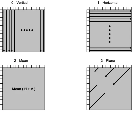
[image:19.612.91.521.440.659.2]2.2.1.1 Intra Prediction
In intra prediction a current macroblock is obtained by using neighboring previously
encoded macroblocks. There is a possibility of Intra prediction occurring at the luma and
sub-block levels. The luma is (16x16) macroblock and sub-block is (4x4) block. The
possible prediction patterns for a sub-block are nine and for macroblocks are four (Figure
5 and Figure 6 respectively). The Encoder is responsible in choosing the optimal intra
prediction pattern. Measuring the Sum of Absolute Errors does this. The prediction
pattern is chosen based on its Sum of absolute errors value. The smaller the value
measured, the better the prediction pattern. The compression rate is also greater when the
value is smaller[3]. After the prediction pattern has been chosen, residual block is obtained
by subtracting the prediction from the current macroblock. The residual blocks are then
2.2.1.2 Inter Prediction
In Inter prediction, prediction macroblock is obtained by using history of previously
encoded frames. This history is stored in the reference frame buffer. The information
about the reference frame is encoded in the bitstream along with the residual. This
information will be used during decoding of the bitstream. The new feature in H.264 is
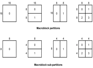
the capability of storing multiple reference frames. Inter prediction uses a 16x16
macroblock that can be partitioned in multiples of 4x4 blocks. As shown in figure 7, the
partitions are tree-structured partitions. The 16 x 16 macroblock can be partitioned into
four 8x8 blocks, which can further be sub-partitioned into four 4x4 blocks. Whenever the
macroblock is partitioned, an additional field is added to the bit-stream that specifies
whether or not and how the sub-block is partitioned. The macroblock when partitioned
also needs to have reference frame number and motion vector that is associated with it.
The reference frame number is to identify which frame the prediction used to calculate
the residual and the motion vector is to identify which sub-block it is. All the blocks
within a partition use the same reference frame but the motion vectors will all be
different. For a 16x16 macroblock partitioned into 4x4 sub-blocks, there will be 16 - 4x4
Figure 8: Tree Structured Macroblock Partitions
The encoder has to optimally partition blocks to balance between the cost of
transmitting/storing motion vectors and the savings of accurate motion prediction that
results in low energy residuals.
frequency data from the frame results in a different image while removal of high
frequency data doesn’t cause much of a difference. Thus the low frequency data is very
important for the frame and has higher priority while the high frequency data is not very
important and has lower priority. This low priority high frequency data can be removed
by using transformation from the spatial domain into frequency domain. H.264 uses
quantization to remove the high frequency data.
The H.264 uses simple 16-bit integer transform. This transform is the integer version of
the Direct Cosine Transform (DCT).
2.2.2.1 4x4 Core Transform and Quantization
H.264 standard uses inter and intra prediction to get prediction of the current macroblock
and to remove temporal and spatial redundancies within a frame. It then subtracts the
prediction obtained from the current macroblock to obtain the residual data. This residual
is then transformed to frequency domain.
€
Y =CfXCfT
Y =
1 1 1 1
2 1 −1 −2 1 −1 −1 1 1 −2 2 −1 ⎡ ⎣ ⎢ ⎢ ⎢ ⎢ ⎤ ⎦ ⎥ ⎥ ⎥ ⎥
X11 X12 X13 X14 X21 X22 X23 X24 X31 X32 X33 X34 X41 X42 X43 X44 ⎡ ⎣ ⎢ ⎢ ⎢ ⎢ ⎤ ⎦ ⎥ ⎥ ⎥ ⎥
1 2 1 1
1 1 −1 −2 1 −1 −1 2 1 −2 1 −1 ⎡ ⎣ ⎢ ⎢ ⎢ ⎢ ⎤ ⎦ ⎥ ⎥ ⎥ ⎥ Eq. 1 X'
=CiTWC i
X'
=
1 1 1 1 2
1 1 2 −1 −1
1 −1 2 −1 1
1 −1 1 −1 2
⎡ ⎣ ⎢ ⎢ ⎢ ⎢ ⎤ ⎦ ⎥ ⎥ ⎥ ⎥ Z11 ' Z12 ' Z13 ' Z14 '
Z21' Z 22 ' Z 23 ' Z 24 '
Z31' Z 32 ' Z 33 ' Z 34 ' Z41 ' Z 42 ' Z 43 ' Z 44 ' ⎡ ⎣ ⎢ ⎢ ⎢ ⎢ ⎤ ⎦ ⎥ ⎥ ⎥ ⎥
1 1 1 1
1 1 2 −1 2 −1
1 −1 −1 1
1 2 −1 1 −1 2
⎡ ⎣ ⎢ ⎢ ⎢ ⎢ ⎤ ⎦ ⎥ ⎥ ⎥ ⎥ Eq. 2
to get inverse core. After applying the core transform the obtained result is passed to the
quantization block, which applies Eq.3 for quantization. In Eq.3, Yij is the value after
applying core transform, PF is a post-scaling factor determined according to Table 2
where and , Qstep is a table look-up factor from Table 3.
€
Zij =round Yij PF Qstep ⎛
⎝ ⎜ ⎜
⎞
⎠ ⎟
⎟ Eq. 3
Position (i,j) PF
(0,0), (2,0), (0,2), (2,2) a2
(1,1), (1,3), (3,1), (3,3) b2/4
else ab/2
Table 2: PF Look-up Table
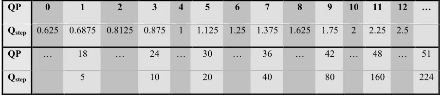
The look-up table, Table.3 facilitates sending the Quantization Parameter (QP) avoiding
fractional numbers.
QP 0 1 2 3 4 5 6 7 8 9 10 11 12 …
Qstep 0.625 0.6875 0.8125 0.875 1 1.125 1.25 1.375 1.625 1.75 2 2.25 2.5
QP … 18 … 24 … 30 … 36 … 42 … 48 … 51
[image:25.612.82.536.528.626.2]2.2.2.2 4x4 and 2x2 Transform for 16x16 Intra Prediction Mode
When the encoder uses 16x16 intra prediction mode then it incorporates two additional
transforms. The core transform is applied 16 times to transform a luma block and 4 times
to transform a chroma block. Thus it applies core transform 24 times to transform a
16x16 macroblock. The core transform applied to luma block 16 times will result 16 DC
luma coefficients (Y11 – Y44 in Eq.4). Then Hadamard transform (Eq.5) is applied to the
16 DC luma coefficients and divided by 2.
€
WD =
1 1 1 1 1 1 −1 −1 1 −1 −1 1 1 −1 1 −1
⎡ ⎣ ⎢ ⎢ ⎢ ⎢ ⎤ ⎦ ⎥ ⎥ ⎥ ⎥
Y11 Y12 Y13 Y14
Y21 Y22 Y23 Y24
Y31 Y32 Y33 Y34 Y41 Y42 Y43 Y44
⎡ ⎣ ⎢ ⎢ ⎢ ⎢ ⎤ ⎦ ⎥ ⎥ ⎥ ⎥
1 1 1 1 1 1 −1 −1 1 −1 −1 1 1 −1 1 −1
⎡ ⎣ ⎢ ⎢ ⎢ ⎢ ⎤ ⎦ ⎥ ⎥ ⎥ ⎥ ⎛ ⎝ ⎜ ⎜ ⎜ ⎜ ⎞ ⎠ ⎟ ⎟ ⎟ ⎟
/2 Eq. 4
€
XD
' =
1 1 1 1
1 1 −1 −1
1 −1 −1 1
1 −1 1 −1
⎡ ⎣ ⎢ ⎢ ⎢ ⎢ ⎤ ⎦ ⎥ ⎥ ⎥ ⎥
Z11' Z 12 ' Z 13 ' Z 14 '
Z21' Z 22 ' Z 23 ' Z 24 ' Z31 ' Z32 ' Z33 ' Z34 '
Z41' Z 42 ' Z 43 ' Z 44 ' ⎡ ⎣ ⎢ ⎢ ⎢ ⎢ ⎤ ⎦ ⎥ ⎥ ⎥ ⎥
1 1 1 1
1 1 −1 −1
1 −1 −1 1
1 −1 1 −1
⎡ ⎣ ⎢ ⎢ ⎢ ⎢ ⎤ ⎦ ⎥ ⎥ ⎥ ⎥ ⎛ ⎝ ⎜ ⎜ ⎜ ⎜ ⎞ ⎠ ⎟ ⎟ ⎟ ⎟ Eq. 5
The core transform applied 4 times to chroma block will result in 4-chroma DC
coefficients ((Y11 – Y22 in Eq.6) and these are sent through Eq.6 and quantized using
€
WD = 1 1
1 −1
⎡
⎣
⎢ ⎤
⎦
⎥ YY11 Y12 21 Y22 ⎡
⎣
⎢ ⎤
⎦ ⎥ 11 1
−1
⎡
⎣
⎢ ⎤
⎦
⎥ Eq. 6
2.2.3 Encoding
In the encoding path after passing transform and quantization block, the macroblock
consists of 24 blocks of which 16 are 4x4 luma coefficient blocks and 8 are 4x4 chroma
coefficient blocks as shown in Figure 9. In addition to these blocks, when 16 x 16 intra
prediction is used there will be additional 4x4 and two 2x2 coefficient blocks. All the
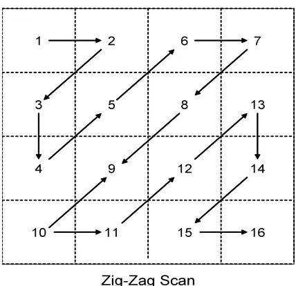
Figure 10: Zig-Zag Scan Order
2.2.3.1 Entropy Coding
H.264 standard defines entropy-coding techniques. They are Context based arithmetic
coding (CABAC), context adaptive variable length coding (CAVLC) and exp-Golomb
entropy coding. This thesis concentrates on the Context adaptive variable length coding
technique and developed a low power VLSI architecture for this algorithm, which is
3 Context Adaptive Variable Length Coding (CAVLC)
This entropy coding technique encodes residual, zigzag ordered 4x4 blocks of transform
coefficients. CAVLC takes advantage of quantized 4x4 blocks.
• After prediction, transformation and quantization blocks typically contain mostly zeros. CAVLC uses run-level coding to compactly represent strings of zeros.
• The highest non-zero coefficients after the zigzag scan are often sequences of +/-1. CAVLC signals the number of Trailing 1s in a compact way.
• The number of non-zero coefficients in neighboring blocks is correlated. The number of coefficients is encoded using a look-up table where the choice of look-up table
depends on the number of non-zero coefficients in neighboring blocks.
• The level or magnitude of non-zero coefficients tends to be higher at the start of the reordered array and lower towards the higher frequencies. CAVLC takes advantage of
this by adapting the choice of VLC look-up table for the level parameter depending
on recently coded level magnitudes.
The context adaptive variable length encoder encodes coefficient token, T1 sign, Level,
3.1 Coefficient token
The coefficient token encodes the total number of non-zero coefficients (TotalCoeffs)
and the number of trailing ones (T1). TotalCoeffs can be anything from 0 to 16. T1 can
be anything from 0 to 3. If there are more than 3 trailing ones, only the last 3 are treated
as trailing ones and any others are coded as normal coefficients. There are 4 choices of
look-up table to use for encoding coefficient token, 3 variable length code tables and a
fixed-length code. The choice of a table depends on the number of non-zero coefficients
in upper and left hand previously coded blocks NA and NB. Parameter, N = (NA +
NB)/2. If only upper block is available then N=NA . If only left hand block is available
then N=NB .If neither is available then N=0.
3.2 T1 sign
The sign of each trailing one signaled by coefficient token is encoded in reverse order,
starting with highest frequency T1. Bit zero is assigned for positive sign one and bit one
for negative sign one.
3.3 Level
The levelof each remaining non-zero coefficient in the block is encoded starting with the
3.4 Total zeros
Total zeros is the sum of all zeros preceding the last non-zero coefficient in the zigzag
ordered array. This sum of all zeros is coded with a VLC.
3.5 Run before
Run before is the number of zeros preceding each non-zero coefficient and this is
4 PROPOSED CAVLC ARCHITECTURE
Figure 11 shows the proposed CAVLC architecture. This architecture is built in software.
It is then simulated to verify correct functionality, and then use Design Compiler to
synthesize the end product. Since Design Compiler cannot synthesize file IO, a test
bench (H264_test) is wrapped around the entire project to do the IO that proved the
functionality. Inside the test bench H264_test, there is the Zigzag scan block, the Ngen
block, Coeff_token, Totalzeros, Level, Run before and Bitstream generator blocks. Input
data to the zigzag scan block is a quantized 4x4 block of coefficients and input to the
Ngen block is the values of NA and NB. The input data to the Zigzag is in the form of a
4x4 array of integers from 0 to 10. Each integer represents a very small image pattern.
4.1 Zigzag Scan Block
The Zigzag block receives the 4x4 arrays of integers. Here, 4 bits are used to store the
integers. Figure 9 shows an example of input data, and how the Zigzag block turns it into
output data. The array of integers is what the Zigzag block receives. The line is the path
that the Zigzag block takes to send the data out. The reason for sending the data like this
is that non-zero integers from the quantization block tend to come in groups. By
performing the Zigzag on this array, more integers are grouped together, and zeroes are
grouped together. After reordering the array the values of Totalcoeffs, T1, T1_sign,
Level, Totalzeros, run before are extracted from the zigzag and reverse ordered array. All
these values are stored in buffers to reduce the dynamic activity. Reduction in dynamic
4.2 Ngen block
There are 4 tables to choose from to encode the Coeff_token (Table 3). 3 tables are
variable length code tables and 1 table is fixed length code table. The choice of the table
depends on the value of N.
€
N =
(
NA +NB)
2 where NA & NB are the number of non-zerocoefficients in upper and left hand previously coded blocks. If only upper block is
available then N=N. If only left hand block is available then N=NB. If neither is available
then N=0. The value of N is generated in this block .The variable length code tables are
biased from small to large number of Totalcoeffs in a block so that smallest code word
can be used for Coeff_token. The fixed length code table is fixed 6-bit code.
N Table for Coeff_token
0,1 Num-VLC0
2,3 Num-VLC1
4,5,6,7 Num-VLC2
8 FLC
Table 4: Coeff_token Look-up Table
4.3 Coeff_token block
The Coeff_token generates the code by reading the values of Totalcoeffs, T1 from the
[image:35.612.231.380.360.483.2]number of trailing ones and the number of non zero coefficients. The flowchart
representing the algorithm for VLC1 is shown in table5. The VLC tables are biased from
small to large number of total nonzero coefficients in a block to facilitate the Coeff_token
to be coded with smallest possible codeword. The output of the Coeff_token block is the
[image:36.612.205.454.209.370.2]length of the Coeff_token and the Coeff_token itself.
Table 5: Coeff_token VLC Table
4.4 Total Zeros block
Totalzeros block encodes the total number of zeros preceding the last nonzero coefficient
in the zigzag array by reading the Totalcoeffs and Totalzeros from the buffers as input.
Case by case code and length are stored in look up tables. Conditional statements are
inserted in the code as shown in table 5 for the look up tables to facilitate clock gating for
low power. Depending on the value of the Totalcoeffs and Totalzeros the code and length
of the code are sent as outputs to the bitstream block. For example if the value of
Totalcoeffs is 7, the value of Totalzeros can range from 0 to 9. So the code and length for
block will be the code output and length depending on the value of the Totalzeros and
[image:37.612.147.465.124.302.2]Totalcoeffs obtained from the zigzag block.
Table 6: Pseudo code for total zeros
4.5 Level block
The level block encodes the nonzero coefficients. The inputs to the block are level and
Totalcoeffs. Totalcoeffs gives the number of nonzero coefficients to be encoded and the
level gives the level of each nonzero coefficient. The format of the level code is the level
prefix followed by bit 1 and that followed by level suffix. Level prefix is the array of
zeros that are in level code and level suffix is the array of bits. The level input is taken for
each nonzero coefficient and this block generates the level prefix, length of level prefix,
level suffix and length of level suffix based on the look up tables which are implemented
using the conditional statements for power reduction. These are then sent to the bitstream
4.6 Run before block
The run before block encodes the number of zeros preceding each nonzero coefficient in
reverse zigzag order by taking the inputs run before, Totalcoeffs and Totalzeros. The
block takes the run before input into an array and Totalzeros into another. It determines
the number of zeros left by subtracting the run before from Totalzeros. Depending on the
value of the zeros left and the run before, the code and the length of the code are
determined from the look up table. The look up table is implemented using conditional
statements to facilitate the clock gating insertion for power reduction. The pseudo code
for the look up table implementation is shown in table 6. The code and length of the code
for run before for each of the nonzero coefficients is sent to the bitstream generator.
4.7 Bitstream generator
The bitstream generator block gets Totalcoeffs, T1’s and Sign inputs from the Zigzag
block; Coefftoken and length of the token from the Coefftoken block; Totalzeros code
and its length from the Totalzeros block; Level suffix, level prefix and their lengths from
the level block; Run before code and its length for each nonzero coefficient from run
before block. The Bitstream generator reads in the inputs and their lengths and appends
5 Simulation and Synthesis Results
The CAVLC architecture was designed and verified with simulations using the Mentor
Graphics Modelsim tools. VHDL code was written to describe the architecture and each
block was verified for functionality with simulations. After verifying the functionality of
each block, all the blocks were wrapped around with the testbench and the test bench was
verified with simulations. A .do file was generated with the clock input and run time for
the simulation. The clock used was of period 10ns for the simulation of the testbench.
The results of the simulation for each block are in the next sections.
5.1 Zigzag Scan Block Simulation
The inputs to the Zigzag block are 16 std_logic_vectors and clock with a 10ns period.
The 16 vectors are then read into 4x4 array and reordered. After reordering the array, the
values of Totalcoeffs, T1, T1_sign, Level, Totalzeros, run before are extracted from the
zigzag and reverse ordered array. Figure 12 shows the simulation results.
5.2 Ngen block Simulation
The inputs to the Ngen block are the values of Na, Nb and NFlag depending on the
algorithm; the value of the N is calculated. Figure 13 shows the simulation results for the
5.3 Coeff_token block Simulation
The inputs to the Coeff_token block are the values of Totalcoeffs, T1 and N value. After
taking these values as inputs, the Coeff_token block implements an algorithm [3] to
represent the VLC tables instead of storing the VLC tables in memory. This block then
outputs the length of the Coeff_token and the Coeff_token itself. Figure 14 shows the
[image:42.612.93.523.281.670.2]simulation result.
5.4 Total Zeros block Simulation
The inputs to the Totalzeros block are the Totalcoeffs and Totalzeros. Totalzeros block
encodes the total number of zeros preceding the last nonzero coefficient in the zigzag
array by taking these inputs. Depending on the value of the Totalcoeffs and Totalzeros
the code and length of the code outputs are generated. Figure 15 shows the simulation
[image:43.612.92.530.242.608.2]5.5 Level block Simulation
The inputs to the level block are level and Totalcoeffs. After taking level input for each
nonzero coefficient, this block outputs the level prefix, length of level prefix, level suffix
[image:44.612.92.527.188.529.2]and length of level suffix. Figure 16 shows the simulation result.
Figure 16: Level simulation.
5.6 Run before block Simulation
The inputs to the run before block are run before, Totalcoeffs and Totalzeros. After
taking these inputs, run before block encodes the number of zeros preceding each
the code for run before for each of the nonzero coefficients are the outputs of this block.
Figure 17 shows the simulation results for this block.
Figure 17: Run before simulation.
5.7 Bitstream generator block Simulation
The inputs to the bitstream generator block are Totalcoeffs, T1’s, Sign inputs,
Coefftoken, length of the token, Totalzeros code, length of Totalzeros code, Level suffix,
length of level suffix, level prefix, length of level prefix, Run before code and its length.
Synopsys Design Compiler was used for the synthesis of the VHDL description of the
CAVLC architecture. Design Compiler was provided with VHDL description of the
functionally verified CAVLC architecture as input along with constraints to generate the
gate level net list. In addition to inputs and design rule constraints, technology and
symbol libraries are needed to generate the net list. The technology libraries specify the
operating conditions and wire load models. The symbol libraries contain the definitions
of the symbols that represent cells in the schematics. The technology library used for the
synthesis of the CAVLC architecture was a 65nm technology library. The synthesized
[image:47.612.94.516.324.671.2]Initially Design compiler was used to carryout a preliminary synthesis to see if the design
meets the basic goals. The design was modified until the desired goals were met and then
Power compiler was used to get the low power design. Power Compiler is used to
minimize power consumption at the RTL and gate level. Power Compiler and Design
Compiler share the same GUI and it is integrated with Design Compiler’s design flow.
There is multiple commonly used power reduction techniques like supply voltage
reduction, clock gating, multi voltage design etc. The most suitable power reduction
technique for this design seemed to be the clock gating technique.
Compiling a design with design compiler usually implements registers with a feedback
loop and a multiplexor. Some of the registers have same value for multiple clock cycles
using power unnecessarily. Clock gating saves power by eliminating the unnecessary
switching on these registers. Clock gating removes the feedback loop and multiplexor
and inserts gates in the clock net of the registers to prevent the clock from clocking the
register. Figure 20 shows a sample schematic before and after clock gating. Significant
6 Results
The proposed architecture designed, simulated and synthesized using a 100MHz clock.
The architecture could encode a 4x4 block in 1200 ns. The performance of the
architecture can be calculated as:
• From Table 1 the number of macroblocks per CIF frame is 396.
• The number of 4x4 blocks per macroblock is 16 assuming the best case with skip mode.
• From above, the total number of 4x4 blocks per CIF frame is 396 x 16 = 6336. • So the time taken to encode a CIF frame would be 6336 x 1200 ns = 7.6 ms. • Therefore the time taken to encode 60 frames would be 60 x 7.6 ms = 456 ms. The designed architecture therefore enables real-time processing for QCIF and CIF
frames with 60-fps using 100MHz clock.
The resultant hardware implementation requires 32K number of logic gates. The resultant
hardware power is 1.4mW. Reference [6] hardware is implemented in Verilog and
synthesized using the Synopsys Design Compiler with TSMC Artisan 0.18µm cell
library. The total power consumption is 3.7mW at 27MHz and 1.8V. The proposed
architecture uses a 100MHz clock whereas the Reference [6] uses 27MHz. Instead of
using a lower clock to decrease the switching activity, this architecture used buffers to
store the symbols and then encoded by reading from the buffers instead of dynamically
encoding the symbols. This helped to reduce the switching and thereby power. To
VHDL description of the CAVLC architecture initially and then power compiler’s clock
gating technique was used for power reduction. Significant improvements in Power were
observed when clock gating was applied by almost 30%. The tool applies clock gating by
finding the conditional statements prior to the assignment statements. This architecture
consists of lot of look up tables and all the look up tables are implemented based on
conditional statements to take advantage of the clock gating. Table 5 shows a comparison
between reference [6], reference [7] and proposed architecture in terms of area, latency,
[image:51.612.116.495.338.495.2]technology library and power.
Table 5: Area, Latency and Technology Comparison.
Design Area Latency Technology library Power
Proposed 32K QCIF and CIF @ 60fps 65nm 1.4mW
Reference [6] 27K QCIF and CIF @ 30fps 0.18um 3.7mW
7 Conclusion
The CAVLC architecture was designed and verified with simulations using the Mentor
Graphics Modelsim tools. VHDL description of the architecture was verified for
functionality with simulation. Synopsys Design Compiler was used for the synthesis of
the VHDL description of the CAVLC architecture initially and then power compiler’s
clock gating technique was used for power reduction. The technology library used for the
synthesis of the CAVLC architecture was a 65nm technology library. Significant
improvements in Power were observed when clock gating was applied by almost 30%.
The designed architecture therefore enables real-time processing for QCIF and CIF
frames with 60-fps using 100MHz clock. The resultant hardware implementation requires
8 Future Work
High Efficiency Video Coding (HEVC) standard is still under development by the ISO
and ITU-T. The Moving Picture Experts Group (MPEG) and Video Coding Experts
Group (VCEG) have set up a Joint Collaborative Team on Video Coding (JCT-VC) with
the aim of getting the new standard ready for publication in 2012/2013 [13]. The
expectation is that it is likely to be published jointly as a new MPEG standard and a new
ITU-T standard, possibly H.265 following the JCT-VC and MPEG meeting in October
2010. According to [13] the new standard there are changes in the Prediction and
transform block sizes and also there will be a Low complexity entropy coding scheme
introduced in this standard which can be implemented in the same way as this proposed
Bibliography
[1] ITU, Telecommunication Standardization Sector, “ITU-T Recommendation H.264”, ITU-T, 2011.
[2] Richardson, Iain E. G., H.264 and MPEG-4 Video Compression, 1 ed., The Atrium, Southern Gate, Chichester, West Sussex PO19 8Sq, England: John Wiley & Sons Ltd., 2003.
[3] Richardson, Iain E. G., “H.264 Intra Prediction”, http://www.codex.com/h264.html, April, 2011.
[4] Richardson, Iain E. G., “H.264 Inter Prediction”, http://www.codex.com/h264.html, April, 2011.
[5] Richardson, Iain E. G., “H.264 Transform”, http://www.codex.com/h.264.html, March, 2011.
[6] Tsai, C., Chen, T., & Chen, L. “LOW POWER ENTROPY CODING
HARDWARE DESIGN FOR H.264/AVC BASELINE PROFILE ENCODER,” in IEEE International conference on Multimedia and Expo, 2006.
[7] T. C. Chen, Y. W. Huang, C. Y. Tsai, B. Y. Hsieh, & L. G. Chen, “Dual-block-pipelined VLSI architecture of entropy coding for H.264/AVC baseline profile,” in Proc. of IEEE VLSI-TSA Int. Symposium on VLSI Design, Automation and Test
(VLSI-TSA-DAT), 2005.
[8] Xiang Li, Novel VLSI Architecture of Motion Estimation and Compensation for H.264 Standard, MS in computer Engineer Thesis, Rochester Institute of Technology, August 3, 2004.
[9] Xiang Li, Kenneth W. Hsu, Rahul Chopra,” An IC Design for Real-Time Motion Estimation for H.264 Digital Video,” in Proc. of IEEE,2005.
[10] Gonzalez, Rafael C., Woods, Richard E., Digital Image Processing, 2 ed., Upper Saddle River, New Jersey 07458: Prentice-Hall Inc., 2002.
[11] Wiegand T., Sullivan G., Bjontegaard G., Lutrha A.: “Overview of the H.264/AVC Video Coding Standard”, IEEE Transactions on Circuits and Systems for Video
Technology, July 2003.
[12] Hong, B., “Introduction to H.264”, Multimedia Communications Laboratory, University of Texas, Nov. 22,
[13] Richardson, Iain. (2012). High Efficiency Video Coding. Retrieved from
![Figure 1: H.264 Baseline Profile Encoder [1].....................................................................](https://thumb-us.123doks.com/thumbv2/123dok_us/110648.10381/5.612.92.523.103.404/figure-h-baseline-profile-encoder.webp)
![Figure 1: H.264 Baseline Profile Encoder [1]](https://thumb-us.123doks.com/thumbv2/123dok_us/110648.10381/11.612.105.510.78.259/figure-h-baseline-profile-encoder.webp)
![Figure 2: Video Compression[1]](https://thumb-us.123doks.com/thumbv2/123dok_us/110648.10381/13.612.93.525.102.234/figure-video-compression.webp)
![Figure 4: Encoder and Decoder[11]](https://thumb-us.123doks.com/thumbv2/123dok_us/110648.10381/17.612.93.523.520.688/figure-encoder-and-decoder.webp)
![Figure 9: 16x16 Macroblock Block Ordering[5]](https://thumb-us.123doks.com/thumbv2/123dok_us/110648.10381/28.612.110.503.68.406/figure-x-macroblock-block-ordering.webp)