Data Descriptor:
A database of
chlorophyll
a
in Australian waters
Claire H. Davieset al.#
Chlorophyllais the most commonly used indicator of phytoplankton biomass in the marine environment. It
is relatively simple and cost effective to measure when compared to phytoplankton abundance and is thus routinely included in many surveys. Here we collate173,333records of chlorophyllacollected since1965 from Australian waters gathered from researchers on regular coastal monitoring surveys and ocean voyages
into a single repository. This dataset includes the chlorophyllavalues as measured from samples analysed
using spectrophotometry,fluorometry and high performance liquid chromatography (HPLC). The Australian
Chlorophylladatabase is freely available through the Australian Ocean Data Network portal (https://portal. aodn.org.au/). These data can be used in isolation as an index of phytoplankton biomass or in combination with other data to provide insight into water quality, ecosystem state, and relationships with other trophic levels such as zooplankton orfish.
Design Type(s) data integration objective • database creation objective
Measurement Type(s) chlorophyll a
Technology Type(s) high performance liquid chromotography assay • fluorometry • spectrophotometry
Factor Type(s) geographic location
Sample Characteristic(s)
phytoplankton • ocean biome • Adelaide • Australia • Bunbury • City of Coffs Harbour • Coorong Lagoon • Darwin • Derwent River • Far North Queensland Area • Great Australian Bight • Great Barrier Reef • Gulf of Carpentaria • Huon River • Kangaroo Island • Kimberley Region • Mackay • Moreton Bay • New South Wales • North West Cape • Queensland • Scott and Seringapatam Reefs • Smith's Lake • South East Queensland Area • South West Region • Southern Ocean • State of Tasmania • State of Victoria • Swan River • Sydney Harbour • Sydney Metropolitan Area • Tasman Sea • Townsville • Western Australia • Wheatbelt Region • Yanchep National Park
Correspondence and requests for materials should be addressed to C.H.D. (email: [email protected]).
#A full list of authors and their affiliations appears at the end of the paper.
OPEN
Received:24August2017
Accepted:5January2018
Background & Summary
As the pigment chlorophyllais present in all photosynthetic phytoplankton species1and is relatively easy and cheap to measure, it has become a standard proxy for estimating phytoplankton biomass2. Samples require minimal processing and storage in the field and are not easily contaminated. Chlorophyll ais cheaper to process using spectrophotometry or fluorometry relative to estimating phytoplankton abundance/biomass using cell counts. Importantly, chlorophyllameasurements also account for the pico and nano plankton in the samples, which are substantially underestimated by phytoplankton analysts using light microscopy. These smaller size classes account for a significant fraction (commonly>70%) of total chlorophyllabiomass3,4.
However, whilst using chlorophyll a as an estimate of phytoplankton biomass is widespread, the relationship between the two variables is complex. Not only does the carbon to chlorophyll ratio of phytoplankton vary with species and morphological characteristics, the chlorophyll a content of a phytoplankton cell per unit of organic matter will vary with light intensity, nutrient availability, temperature and cell age5–8. Despite these complexities chlorophyllaremains useful as a coarse proxy for phytoplankton biomass.
In Australian waters chlorophyllaconcentrations are generally lowest in the tropical and subtropical oceanic regions (0.05-0.5μgL−1) and higher in the Southern Ocean and temperate regions (up to 1.5
μgL−1)2. In coastal zones, the chlorophyllaconcentration canfluctuate greatly as phytoplankton blooms develop, peak and crash. The coastal station at Port Hacking, project number P782 in our database, is a good example where chlorophyllaconcentrations typically vary between 0.1–8.0μgL−1over an annual cycle, with peaks sometimes up to 15μgL−1at 20–40 m depth coinciding with phytoplankton blooms9. In inshore estuaries and bays, high chlorophyll a values can also indicate the system is eutrophic with elevated nutrient levels from terrestrial run off. Chlorophyllais therefore used in several water quality monitoring programs across the country (e.g. project number P1072 Ecosystem Health Monitoring Program in Moreton Bay, Queensland, Australia, http://healthywaterways.org/initatives/monitoring). Concentrations of chlorophyll aalso vary throughout the oceans with oceanographic features such as upwelling and fronts which drive nutrients towards surface layers and thus enhance chlorophyll a levels10,11.
Here we collate all available chlorophylla data from Australian waters, gathered from researchers, students, government bodies, state agencies, councils and databases, along with the associated metadata through the process as detailed in Fig. 1. The chlorophyllavalues are as measured and no attempt has been made to synthesise the data across analysis methods. The Australian Chlorophyll a database is available through the Australian Ocean Data Network portal (AODN: https://portal.aodn.org.au/), the main repository for marine data in Australia. The Australian ChlorophyllaDatabase will be maintained and updated through the CSIRO data centre, with periodic updates sent to the AODN. A snapshot of the Australian ChlorophyllaDatabase at the time of this publication has been assigned a DOI and will be maintained in perpetuity by the AODN (Data Citation 1).
Methods
There are three standard methods for determining chlorophyll a concentrations in water samples: spectrophotometry, fluorometry and high performance liquid chromatography (HPLC). Spectro-photometric methods are described fully in Strickland and Parsons (1972)12, fluorometry in Zeng (2015)13, and HPLC in Shoaf (1978)14. A comprehensive discussion of the details of each method and its
merits can be found in Manoturaet al.(1997) and Royet al.(2011)15,16.
To measure chlorophylla, a known volume of water sample isfiltered through a glassfibrefilter paper, typically 0.45-0.7μm pore size, under a gentle vacuum. The volume filtered varies depending on the chlorophyllaconcentration expected in the sample, with more waterfiltered at lower concentrations, but the volume should be sufficient to produce a green tinge on thefilter paper. Chlorophyllais extracted from the filter paper with an organic solvent (e.g. acetone). Concentrations are derived from a spectrophotometer to record the light absorbance at particular wavelengths or a fluorometer that transmits an excitation beam of light in the blue range (440–460 nm) and detects the lightfluoresced by chlorophyllain the red wavelength range (650–700 nm). Thisfluorescence is directly proportional to the concentration of chlorophylla. For HPLC, thefilter paper is similarly extracted with an organic solvent, however pigments are then separated by passing the extract through a chromatographic column and then measured either spectrophotometrically orfluorometrically.
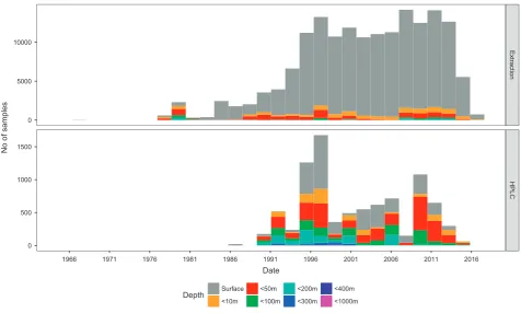
Although HPLC has become the accepted benchmark for the quantification of chlorophyll a the volume of data collated in this database shows that spectrophotometric and fluorometric extraction methods are much more commonly used (Fig. 2). HPLC has the advantages of being more accurate and also quantifies all the other accessory pigments but it does require specialised equipment and technical skills which make it more expensive. Spectrophotometry andfluorometry are simpler and effective, but unlike HPLC they do not differentiate between chlorophyll functional types and accessory pigments. To improve the spectrophotometric and fluorometric methods, an acidifying step (e.g. addition of a small amount of hydrochloric acid) can be added after the extraction to reduce errors associated with chlorophyll degradation products2.
current dataset because chlorophyll a estimates from in-situ fluorometers are notoriously difficult to calibrate to an absolute standard. Although the accuracy of fluorometers is continually improving they require regular calibration, including against other methods13. The instruments are somewhat unstable and measurements are influenced by the presence of other environmental factors, particularly coloured dissolved organic matter (CDOM), diel, seasonal and regional effects and would also require correction for these factors13. The calibration routines must account for physical factors such as sensor drift,
instrument design, biofouling etc. as well as the phytoplankton community composition and physiology in the sample environment, which may vary over space and time.
[image:3.595.157.493.51.197.2]Data collated for this database have come from many different sources, from long-term monitoring programs run by local governments concerned with water quality to ocean voyages on research vessels. Data have been standardised toμgL−1, and the collection and analysis methods have been included so that inter-project comparisons can be considered. We have collated data from researchers, local and state government agencies and regional databases, e.g. AESOP (The Australian-waters Earth Observation Phytoplankton-type products) database (http://aesop.csiro.au/). The database will be maintained by the CSIRO Data Centre and updates will be available periodically through the AODN.
Figure 1. Flow diagram of data collation, verification and release to AODN.
Extr
action
HPLC
1966 1971 1976 1981 1986 1991 1996 2001 2006 2011 2016
0 5000 10000
0 500 1000 1500
Date
No of samples
Depth Surface <10m
<50m <100m
<200m <300m
<400m <1000m
[image:3.595.84.561.242.528.2]Data Records
Each data record represents the chlorophyllameasurement taken at a point in space and time and has a unique record identification number, P(project_id)_(sample_id)_(record_id). Each data record belongs
110°E 120°E 130°E 140°E 150°E 160°E 170°E 180°
70 ° S6 0° S5 0° S4 0° S3 0° S2 0° S1 0° S
110°E 120°E 130°E 140°E 150°E 160°E 170°E 180°
70 ° S6 0 ° S5 0 ° S4 0 ° S3 0 ° S2 0 ° S1 0 ° S
786; 788; 793; 995; 1050; 1053, 1134 990
972 1013; 1069; 1133 988 971 996; 1025; 1027 1063 986 978; 1051 1007 796 999 985 969; 1084 479; 591; 979; 1114 599
980; 993; 1002; 1006; 1015; 1020; 1022; 1024; 1082; 1113 1127
110°E 120°E 130°E 140°E 150°E 160°E 170°E 180°
70° S6 0° S5 0° S4 0° S3 0° S2 0° S1 0° S
110°E 120°E 130°E 140°E 150°E 160°E 170°E 180°
70 ° S6 0 ° S5 0 ° S4 0 ° S3 0 ° S2 0 ° S1 0 ° S 1053; 1130 1013; 1069; 1133 589 1071; 1073; 1074 1058 1062 1060 1061 1075 1055 1072 1065 1059 797 782
[image:4.595.135.536.48.642.2]479; 591; 979; 1114 609 509 1076 806 1077 6 4 17 7 1080 1081 1122 1124 1125 1126 1128 1129 1064 1031
Figure 3. Sample locations mapped by analysis type, by HPLC and by spectrophotometry and
to a project, with each project having a unique identification number, Pxxx. A project is defined as a set of data records that have been collected together, usually as a cruise or study, and have the same sampling and analysis methods and the same person analysing the samples. Metadata ascribed to a project relates to all data records within that project. Details to identify each project, along with their associated samples, time and space information (Table 1 (available online only), Fig. 3) allow users to select and download discrete datasets in their area of interest. While each sample within a project has a unique sample_id, there may be more than one chlorophyll a record per sample if multiple replicates or depths were sampled. The sample_id has not been changed from the original data set to maintain traceability. Therefore P(project_id)_(sample_id) may be duplicated within projects, but the chlorophyll arecords within that sample, taken at different depths for example, are given a unique record_id.
Each data record has been quality controlled. Data with insufficient or unreliable metadata were removed. All depths, times and locations have been validated and are within the boundaries expected for each project.
Technical Validation
The database has been constructed to ensure data extraction is straight forward, although the user needs to be aware of two caveats. First, if chlorophyllbor other pigments are present, thenfluorometry may underestimate or spectrophotometry overestimate the chlorophyllaconcentration relative to HPLC17–19. When an acidification step is included, the accuracy of chlorophyll a from spectrophotometric and
fluorometric methods is improved as effects of chlorophyll degradation products are reduced18. Without further pigment information comparisons between methods need to be carefully considered. This database reports values as measured and does not attempt to compare values across methods, leaving this to the discretion of the user. Second, for the HPLC data we are reporting the sum of the chlorophylla pigments including the divinyl chlorophyll a components. The user should thus be careful when comparing data across datasets where different analysis methods have been used. Metadata have been provided in as much detail as is available so the user is aware of methodological details specific to the project.
Chlorophylla values can be reported in micrograms per litre (μgL−1), milligrams per cubic metre
(mgm−3) (1μgL−1=1 mgm−3) or as depth integrated values, i.e. per square metre (mgm−2). In this data set we have standardised to μgL−1. Where depth integrated values were given, the appropriate sample depth from the study was used to convert toμgL−1.
All times have been converted to Coordinated Universal Time, UTC. Dates with no time component remain as reported.
The value−999 has been assigned to values that were below detection limits. The detection limit has also been included, where known, in the sample_methodfield of the metadata table.
Usage Notes
This dataset and metadata has been made freely available through the AODN (Data Citation 1). The Australian Chlorophylladatabase is complementary to the Australian Zooplankton Database20and the Australian Phytoplankton Database21, both of which provide species-level data and are available through the AODN. Many projects in this data set have corresponding data in these species level databases and can be matched to the project via Project_id and to individual samples, via sample_id, or by using the time and date information. For example, the project 599 has data on zooplankton and phytoplankton composition, included in the aforementioned databases, plus chlorophylladata in the current data set. Because the three data sets were collected at the same locations and times as part of the Integrated Marine Observing System (IMOS) National Reference Stations (NRS), they can be analysed together to investigate relationships among different trophic levels. These combined data have been used in an analysis of climate-driven variability contrasting the 2010 El Niño with the 2011 La Niña22. Further examples of using chlorophyll data in partnership with species-level phytoplankton and zooplankton data using data are from project 17 in the North West Cape, Western Australia23,24.
Projects 599, 1063, 1064, 1065, 1071, 1072, 1074, 1078 and 1129 are ongoing, and data will continue to be added to the Australian chlorophylladatabase; for further information, contact the data custodian as listed in the metadata. The most updated version of P599 IMOS National Reference Stations, is available at: https://portal.aodn.org.au/search?uuid=f48531e2-f182-56ca-e043-08114f8c7f2e.
References
1. Jeffrey, S. W inPrimary Productivity in the Sea. ed. (Paul G.Falkowski) 33–58 (Springer: US, 1980). 2. Jeffrey, S. W. & Hallegraeff, G. M inBiology of marine plantsCh. 14, 310–348 (Longman, 1990).
3. Maranon, E.et al.Patterns of phytoplankton size structure and productivity in contrasting open-ocean environments.Marine Ecology Progress Series216,43–56 (2001).
4. Buitenhuis, E. T.et al.Picophytoplankton biomass distribution in the global ocean.Earth System Science Data4,37–46 (2012). 5. Hallegraeff, G. M. Comparison of different methods used for quantitative-evaluation of biomass of freshwater phytoplankton.
Hydrobiologia55,145–165 (1977).
6. Jakobsen, H. H. & Markager, S. Carbon-to-chlorophyll ratio for phytoplankton in temperate coastal waters: Seasonal patterns and relationship to nutrients.Limnology and Oceanography61,1853–1868 (2016).
7. Menden-Deuer, S. & Lessard, E. J. Carbon to volume relationships for dinoflagellates, diatoms, and other protist plankton.
8. Roy, S., Sathyendranath, S. & Platt, T. Size-partitioned phytoplankton carbon and carbon-to-chlorophyll ratio from ocean colour by an absorption-based bio-optical algorithm.Remote Sensing of Environment194,177–189 (2017).
9. Hallegraeff, G. M. Seasonal Study of Phytoplankton Pigments and Species at a Coastal Station off Sydney: Importance of Diatoms and the Nanoplankton.Mar. Biol.61,2–3 (1981).
10. Ajani, P.et al.Establishing baselines: a review of eighty years of phytoplankton diversity and biomass in southeastern Australia.
Oceanography and Marine Biology54,387–412 (2016).
11. Armbrecht, L. H.et al.Phytoplankton composition under contrasting oceanographic conditions: Upwelling and downwelling (Eastern Australia).Continental Shelf Research75,54–67 (2014).
12. Strickland, J. D. H. & Parsons, T. R.A practical handbook of seawater analysis. 2 edn, 310 (Fisheries Research Board of Canada, 1972).
13. Zeng, L. H. & Li, D. L. Development of In Situ Sensors for Chlorophyll Concentration Measurement.Journal of Sensors2015,
16 (2015).
14. Shoaf, W. T. Rapid method for separation of chlorophylis-a and chlorophylis-b by high-pressure liquid-chromatography.Journal of Chromatography152,247–249 (1978).
15. Mantoura, R., Jeffrey, S. W., Llewellyn, C. A., Claustre, H., Morales, C. E. inPhytoplankton pigments in oceanographyeds (Jeffrey S. W., Mantoura R.F.C. & Wright S.W.) Ch. 14, 361–380 (UNESCO, 1997).
16. Roy, S., Llewellyn, C. A., Egeland, E. S. & Johnsen, G.Phytoplankton pigments: characterization, chemotaxonomy and applications in oceanography(Cambridge University Press, 2011).
17. Pinckney, J., Papa, R. & Zingmark, R. Comparison of high-performance liquid-chromatographic, spectrophotometric, and
fluorometric methods for determining chlorophyll a concentrations in estuarine sediments.Journal of Microbiological Methods 19,59–66 (1994).
18. Daemen, E. Comparison of methods for the determination of chlorophyll in estuarine sediments.Netherlands Journal of Sea Research20,21–28 (1986).
19. Murray, A. P., Gibbs, C. F., Longmore, A. R. & Flett, D. J. Determination of chlorophyll in marine waters-intercomparison of a rapid HPLC method with full HPLC, spectrophotometric andfluorometric methods.Marine Chemistry19,211–227 (1986). 20. Davies, C. H.et al.Over 75 years of zooplankton data from Australia.Ecology95,3229–3229 (2014).
21. Davies, C. H.et al.A database of marine phytoplankton abundance, biomass and species composition in Australian waters.
Scientific Data3(2016).
22. Thompson, P. A.et al.Climate variability drives plankton community composition changes: the 2010-2011 El Nino to La Nina transition around Australia.Journal of Plankton Research37,966–984 (2015).
23. Furnas, M. Intra-seasonal and inter-annual variations in phytoplankton biomass, primary production and bacterial production at North West Cape, Western Australia: Links to the 1997-1998 El Nino event.Continental Shelf Research27,958–980 (2007). 24. McKinnon, A. D., Duggan, S., Carleton, J. H. & Bottger-Schnack, R. Summer planktonic copepod communities of Australia's
North West Cape (Indian Ocean) during the 1997-99 El Nino/La Nina.Journal of Plankton Research30,839–855 (2008). 25. Wright, S. Aurora Australis Voyage 6 (SAZ Subantarctic Zone) 199798 Chlorophyll a Data Australian Antarctic Data Centre
-CAASM Metadata https://data.aad.gov.au/metadata/records/SAZ_Chlorophyll (2014).
26. Raes, E. J.et al.Sources of new nitrogen in the Indian Ocean.Global Biogeochemical Cycles29,1283–1297 (2015).
27. Raes, E. J.et al.Changes in latitude and dominant diazotrophic community alter N-2fixation.Marine Ecology Progress Series516,
85–102 (2014).
28. Waite, A. M.et al.Cross-shelf transport, oxygen depletion, and nitrate release within a forming mesoscale eddy in the eastern Indian Ocean.Limnology and Oceanography61,103–121 (2016).
29. McKinnon, A., Duggan, S., Böttger-Schnack, R., Gusmão, L. & O'Leary, R. Depth structuring of pelagic copepod biodiversity in waters adjacent to an Eastern Indian Ocean coral reef.Journal of Natural History47,639–665 (2013).
30. Wright, S. Role of Antarctic marine protists in trophodynamics and global change and impact of UV-B on these organisms - V1 of the Aurora Australis, 1995-96 - HI-HO, HI-HO Australian Antarctic Data Centre - CAASM Metadata https://data.aad.gov.au/ metadata/records/ASAC_40_HIHOHIHO (2016).
31. Wright, S.Nella Dan: ADBEX I Cruise - Chlorophyll a data Australian Antarctic Data Centre - CAASM Metadatahttps://data.aad. gov.au/metadata/records/ADBEX_I_Chlorophyll (2014).
32. Wright, S.Aurora Australis Voyage 2 (ONICE) 1997-98 Chlorophyll a Data Australian Antarctic Data Centre-CAASM Metadata
https://data.aad.gov.au/metadata/records/ONICE_Chlorophyll (2014).
33. Wright, S.Aurora Australis Voyage 6 (FISHOG) 199192 Heard Island Chlorophyll a Data Australian Antarctic Data Centre -CAASM Metadatahttps://data.aad.gov.au/metadata/records/AADC-00094 (2014).
34. Wright, S.Aurora Australis Voyage 7 (KROCK) 1992-93 Chlorophyll a Data Australian Antarctic Data Centre - CAASM Metadata
https://data.aad.gov.au/metadata/records/AADC-00096 (2014).
35. Wright, S.Chlorophyll a data collected on voyage 4 of the Aurora Australis in the 1991-1992 season Australian Antarctic Data Centre-CAASM Metadatahttps://data.aad.gov.au/metadata/records/199192040_Chlorophyll (2014).
36. Wright, S.Chlorophyll a data collected on the AAMBER II cruise of the Aurora Australis Australian Antarctic Data Centre -CAASM Metadatahttps://data.aad.gov.au/metadata/records/AAMBER_II_Chlorophyll (2014).
37. Wright, S.Aurora Australis Voyage 9 (WOES) 1992-93 Chlorophyll a Data Australian Antarctic Data Centre - CAASM Metadata
https://data.aad.gov.au/metadata/records/WOES_Chlorophyll (2014).
38. McKinnon, A. D., Duggan, S., Holliday, D. & Brinkman, R. Plankton community structure and connectivity in the Kimberley-Browse region of NW Australia.Estuarine Coastal and Shelf Science153,156–167 (2015).
39. Dela-Cruz, J., Middleton, J. H. & Suthers, I. M. The influence of upwelling, coastal currents and water temperature on the distribution of the red tide dinoflagellate, Noctiluca scintillans, along the east coast of Australia.Hydrobiologia598,59–75 (2008). 40. Dela-Cruz, J., Middleton, J. H. & Suthers, I. M. Population growth and transport of the red tide dinoflagellate, Noctiluca
scintillans, in the coastal waters off Sydney Australia, using cell diameter as a tracer.Limnology and Oceanography48,
656–674 (2003).
41. Burford, M. A.et al.Controls on phytoplankton productivity in a wet-dry tropical estuary.Estuarine Coastal and Shelf Science 113,141–151 (2012).
42. Everett, J. D. & Doblin, M. A. Characterising primary productivity measurements across a dynamic western boundary current region.Deep-Sea Research Part I-Oceanographic Research Papers100,105–116 (2015).
43. Burford, M. A., Rothlisberg, P. C. & Wang, Y. G. Spatial and temporal distribution of tropical phytoplankton species and biomass in the Gulf of Carpentaria, Australia.Marine Ecology Progress Series118,255–266 (1995).
44. Rothlisberg, P.et al.Phytoplankton community structure and productivity in relation to the hydrological regime of the Gulf of Carpentaria, Australia, in summer.Marine and Freshwater Research45,265–282 (1994).
45. Burford, M. & Rothlisberg, P. Factors limiting phytoplankton production in a tropical continental shelf ecosystem.Estuarine, Coastal and Shelf Science48,541–549 (1999).
47. Henschke, N., Everett, J. D., Baird, M. E., Taylor, M. D. & Suthers, I. M. Distribution of life-history stages of the salp Thalia democratica in shelf waters during a spring bloom.Marine Ecology Progress Series430,49–62 (2011).
48. Henschke, N.et al.Demography and interannual variability of salp swarms (Thalia democratica).Marine Biology161,
149–163 (2014).
49. Robinson, C. M.et al.Phytoplankton absorption predicts patterns in primary productivity in Australian coastal shelf waters.
Estuarine Coastal and Shelf Science192,1–16 (2017).
Data Citation
1. Davies, C. H.et al. Australian Ocean Data Networkhttp://dx.doi.org/10.4225/69/586f220c3f708 (2017).
Acknowledgements
We acknowledge the contributions from all collaborators and their institutions. If data from multiple projects are used, please acknowledge this publication; if individual project data are used, please acknowledge use of data as per the custodian information. We would also encourage data users to enter into collaboration with the researchers involved in the data they use–understanding the history of a project will add value to your research. The relevant acknowledgement data is available from the metadatafiles attached to the data. If using data from Project 599 the National Reference Stations please use the following acknowledgement: “Data sourced from the Integrated Marine Observing System (IMOS) – IMOS is a national collaborative research infrastructure, supported by the Australian Government. It is operated by a consortium of institutions as an unincorporated joint venture, with the University of Tasmania as Lead Agent.” Similarly, for Project 806, please use the following acknowledgement: “A part of the data included in the database was obtained with support from the Great Barrier Reef Marine Park Authority, through funding from the Australian Government Reef Program and from the Australian Institute of Marine Science”. For Project 1129 the information is supplied on the condition that if used in a study or publication the Department of Water is acknowledged as the source of the information. Citations may take the following form:
•Water INformation (WIN) database - discrete sample data. [10-04-2017]. Department of Water, Water Information section, Perth Western Australia.
Author Contributions
C.H.D. collated data, built the database and wrote the manuscript. A.J.R. conceived the study and provided input into the manuscript. S.E. and M.M. provided database support and set up the web server export to the AODN. R.P. (AODN), N.A. and X.H. represent the AODN. Further data regarding specific author input from several projects can be found in Table 1 (available online only).
Additional Information
Table 1 is only available in the online version of this paper.
Competing interests: The authors declare no competingfinancial interests.
How to cite this article: Davies, C. H. et al. A database of chlorophyllain Australian waters.Sci. Data 5:180018 doi: 10.1038/sdata.2017.18 (2018).
Publisher’s note:Springer Nature remains neutral with regard to jurisdictional claims in published maps and institutional affiliations.
Open AccessThis article is licensed under a Creative Commons Attribution 4.0 Interna-tional License, which permits use, sharing, adaptation, distribution and reproduction in any medium or format, as long as you give appropriate credit to the original author(s) and the source, provide a link to the Creative Commons license, and indicate if changes were made. The images or other third party material in this article are included in the article’s Creative Commons license, unless indicated otherwise in a credit line to the material. If material is not included in the article’s Creative Commons license and your intended use is not permitted by statutory regulation or exceeds the permitted use, you will need to obtain permission directly from the copyright holder. To view a copy of this license, visit http://creativecommons. org/licenses/by/4.0/
The Creative Commons Public Domain Dedication waiver http://creativecommons.org/publicdomain/ zero/1.0/ applies to the metadatafiles made available in this article.
Claire H. Davies1, Penelope Ajani2, Linda Armbrecht3, Natalia Atkins4, Mark E. Baird1, Jason Beard5,
Pru Bonham1, Michele Burford6, Lesley Clementson1, Peter Coad7, Christine Crawford5,
Jocelyn Dela-Cruz8, Martina A. Doblin2, Steven Edgar9, Ruth Eriksen1,10, Jason D. Everett11,
Miles Furnas12, Daniel P. Harrison13, Christel Hassler14, Natasha Henschke15, Xavier Hoenner4,
Tim Ingleton8, Ian Jameson16, John Keesing17, Sophie C. Leterme18, M James McLaughlin17,
Margaret Miller9, David Moffatt19, Andrew Moss20, Sasi Nayar21, Nicole L. Patten21, Renee Patten22,
Sarah A. Pausina9,23, Roger Proctor4, Eric Raes24,25, Malcolm Robb26, Peter Rothlisberg9,
Emily A. Saeck6, Peter Scanes27, Iain M. Suthers11,13, Kerrie M. Swadling5,10, Samantha Talbot12,
Peter Thompson1, Paul G. Thomson28, Julian Uribe-Palomino9, Paul van Ruth21, Anya M. Waite24,25,
Simon Wright29& Anthony J. Richardson9,30
1CSIRO Oceans and Atmosphere, Castray Esplanade, Hobart, TAS7000, Australia.2Climate Change
Cluster (C3), University of Technology Sydney, Broadway, NSW 2007, Australia. 3Department of
Biological Sciences, Marine Research Centre, Macquarie University, North Ryde, NSW 2109,
Australia. 4Australian Ocean Data Network, Integrated Marine Observing System University of
Tasmania, Hobart, Tasmania,7001, Australia.5Institute for Marine and Antarctic Studies, University
of Tasmania, TAS7001, Australia.6Australian Rivers Institute, Griffith University, Nathan, QLD4111,
Australia. 7Natural Resources, Hornsby Shire Council, Hornsby NSW 2077, Australia. 8Waters,
Wetlands and Coasts Science Branch, NSW Office of Environment and Heritage, Sydney South, NSW
1232, Australia. 9CSIRO Oceans and Atmosphere, EcoSciences Precinct, Dutton Park, QLD 4102,
Australia. 10Antarctic Climate and Ecosystems Cooperative Research Centre, Hobart, TAS 7001,
Australia. 11Evolution and Ecology Research Centre, University of New South Wales, Sydney, NSW
2052, Australia.12Australian Institute of Marine Science, Townsville, QLD4810, Australia.13Sydney
Institute of Marine Science, Mosman, NSW 2088, Australia. 14Department F.-A. Forel for
Environmental and Aquatic Sciences, Earth and Environmental Sciences, University of Geneva,
Geneva 4, Switzerland. 15Department of Earth, Ocean and Atmospheric Sciences, University of
British Columbia, Columbia, Canada.16CSIRO National Collections and Marine Infrastructure, Castray
Esplanade, Hobart, TAS 7000, Australia. 17CSIRO Oceans and Atmosphere, Indian Ocean Marine
Research Centre (UWA), Crawley, WA 6009, Australia. 18School of Biological Sciences, Flinders
University, Adelaide, SA 5001, Australia.19Ecosystem Health Monitoring Program, Department of
Science, Information Technology and Innovation, Brisbane QLD 4001, Australia. 20Environmental
Monitoring and Assessment Sciences, Science Division, Department of Science, Information
Technology and Innovation, Brisbane QLD 4001, Australia. 21South Australian Research and
Development Institute – Aquatic Sciences, Henley Beach, SA 5022, Australia. 22Environment
Protection Authority, Centre for Applied Science, Ernest Jones Drive, Macleod, VIC3085, Australia.
23School of Biological Sciences, The University of Queensland, St Lucia Qld4072, Australia.24School
of Civil, Environmental and Mining Engineering and the UWA Oceans Institute, The University of
Western Australia, Crawley, WA 6009, Australia. 25Alfred Wegener Institute, Helmholz Centre for
Polar and Marine Research, Am Handelshafen12, D-27570Bremerhaven and University of Bremen,
28359 Bremen, Germany. 26Department of Water, Water Information and Modelling, Georges
Terrace Perth, Australia. 27Estuary and Catchment Science, NSW Office of Environment and
Heritage, Sydney South, NSW 1232, Australia. 28Ocean Graduate School and the UWA Oceans
Institute, The University of Western Australia, Crawley, WA 6009, Australia. 29Southern Ocean
Ecosystem Change program, Australian Antarctic Division and Antarctic Climate and Ecosystems
Cooperative Research Centre, 203 Channel Hwy Kingston, Tas 7050 Australia. 30Centre for
Applications in Natural Resource Mathematics (CARM), School of Mathematics and Physics, The