Making ecological indicators management ready: assessing the specificity, sensitivity, and threshold response of ecological indicators

Contents lists available atScienceDirect

Ecological Indicators

journal homepage:www.elsevier.com/locate/ecolind

Original Articles

Making ecological indicators management ready: Assessing the specificity,

sensitivity, and threshold response of ecological indicators

Caihong Fu

_{, Yi Xu}

_{, Alida Bundy}

_{, Arnaud Grüss}

_{, Marta Coll}

_{, Johanna J. Heymans}

_,

Elizabeth A. Fulton

_{, Lynne Shannon}

_{, Ghassen Halouani}

_{, Laure Velez}

_{, Ekin Akoglu}

_,

Christopher P. Lynam

_{, Yunne-Jai Shin}

a_{Pacific Biological Station, Fisheries and Oceans Canada, 3190 Hammond Bay Road, Nanaimo, BC, V9T 6N7, Canada} b_{Bedford Institute of Oceanography, Fisheries and Oceans Canada, PO Box 1006, Dartmouth, NS B2Y 4A2, Canada} c_{School of Aquatic and Fishery Sciences, University of Washington, Box 355020, Seattle, WA 98105-5020, USA}

d_{Institute of Marine Science (ICM-CSIC), Passeig Maritim de la Barceloneta, n° 37-49. 08003 & Ecopath International Initiative Research Association, Barcelona, Spain} e_{Scottish Association for Marine Science, Scottish Marine Institute, Oban, Argyll PA371QA, UK}

f_{European Marine Board, Wandelaarkaai 7, Oostende 8400, Belgium} g_{CSIRO Oceans & Atmosphere, GPO Box 1538, Hobart, TAS 7001, Australia} h_{Centre for Marine Socioecology, University of Tasmania, Hobart, TAS, Australia}

i_{Department of Biological Sciences, and Marine Research Institute, University of Cape Town, Private Bag X3, Rondebosch, 7701, South Africa} j_{Marine and Freshwater Research Centre (MFRC), Galway-Mayo Institute of Technology (GMIT), Dublin Road, Galway, Ireland}

k_{Institut de Recherche pour le Développement, UMR MARBEC (IRD, University Montpellier, Ifremer, CNRS), Montpellier, France} l_{Middle East Technical University, Institute of Marine Sciences, 33731 Erdemli, Turkey}

m_{Istituto Nazionale di Oceanografia e di Geofisica Sperimentale, Borgo Grotta Gigante 42/C, 34010 Sgonico, TS, Italy}

n_{Centre for Environment, Fisheries and Aquaculture Science (Cefas), Lowestoft Laboratory, Pakefield Road, Lowestoft, Suffolk NR33 0HT, UK}

A R T I C L E I N F O

Keywords:

Ecological modelling Fishing pressure Gradient forest method Indictor performance Marine ecosystem Primary productivity

A B S T R A C T

Moving toward ecosystem-based fisheries management (EBFM) necessitates a suite of ecological indicators that are responsive to fishing pressure, capable of tracking changes in the state of marine ecosystems, and related to management objectives. In this study, we employed the gradient forest method to assess the performance of 14 key ecological indicators in terms of specificity, sensitivity and the detection of thresholds for EBFM across ten marine ecosystems using four modelling frameworks (Ecopath with Ecosim, OSMOSE, Atlantis, and a multi-species size-spectrum model). Across seven of the ten ecosystems, high specificity to fishing pressure was found for most of the 14 indicators. The indicators biomass to fisheries catch ratio (B/C), mean lifespan and trophic level of fish community were found to have wide utility for evaluating fishing impacts. The biomass indicators, which have been identified as Essential Ocean Variables by the Global Ocean Observing System (GOOS), had lower performance for evaluating fishing impacts, yet they were most sensitive to changes in primary pro-ductivity. The indicator B/C was most sensitive to low levels of fishing pressure with a generally consistent threshold response around 0.4*FMSY(fishing mortality rate at maximum sustainable yield) across nine of the ten ecosystems. Over 50% of the 14 indicators had threshold responses at, or below ∼0.6*FMSYfor most ecosystems, indicating that these ecosystems would have already crossed a threshold for most indicators when fished atFMSY. This research provides useful insights on the performance of indicators, which contribute to facilitating the worldwide move toward EBFM.

1. Introduction

Marine ecosystem status and functioning are influenced by various anthropogenic and environmental stressors that necessitate

ecosystem-based, integrative approaches to fisheries management (Garcia et al., 2003; Link et al., 2010; Stephenson et al., 2018). Moving toward eco-system-based fisheries management (EBFM) requires decision-making to be supported by a suite of ecological indicators that are responsive to

https://doi.org/10.1016/j.ecolind.2019.05.055

Received 9 January 2019; Received in revised form 14 May 2019; Accepted 21 May 2019 ⁎_{Corresponding author.}

E-mail addresses:[email protected](C. Fu),[email protected](Y. Xu),[email protected](A. Bundy),

[email protected](E.A. Fulton),[email protected](L. Shannon),[email protected](C.P. Lynam),[email protected](Y.-J. Shin). 1_{Present address: Fraser River and Interior Area Stock Assessment, Fisheries and Oceans Canada, 3-100 Annacis Parkway, Delta, BC V3M 6A2, Canada.}

Ecological Indicators 105 (2019) 16–28

Available online 28 May 2019

1470-160X/ © 2019 The Authors. Published by Elsevier Ltd. This is an open access article under the CC BY-NC-ND license (http://creativecommons.org/licenses/BY-NC-ND/4.0/).

fishing pressure, capable of tracking changes in the state of marine ecosystems and their emergent properties, and related to fisheries management objectives (Bundy et al., 2012; Greenstreet et al., 2012; Piet and Hintzen, 2012; Probst et al., 2013; Shin et al., 2018). A large number of ecological indicators have been documented and reported worldwide, and an increasing number of studies has been conducted to assess the properties of ecological indicators and determine how they should be selected for assisting fisheries management (e.g. Rice and Rochet 2005; Shin et al., 2010; Kershner et al., 2011; Houle et al., 2012; Heymans et al., 2014; Otto et al., 2018). Importantly, the performance of indicators should be evaluated in terms of their response to changes in fishing pressure and other potential drivers in marine ecosystems (Shin et al., 2012, 2018; Hunsicker et al., 2016).

Recent comprehensive studies of exploited marine ecosystems sug-gested that detailed information about past and present fishery ex-ploitation strategies, mechanisms of productivity dynamics, and the dominant ecological and environmental features were essential to cor-rectly interpret ecological indicators in relation to the status of exploited marine ecosystems (e.g. Link et al., 2010; Shannon et al., 2014; Fu et al., 2015; Heymans and Tomczak, 2016). In short, the presence of multiple drivers impacting ecosystems and the diverse ecological and environmental features as well as unique exploitation history of an ecosystem emphasize the need to investigate the responses of indicators to different individual stressors, as well as multiple-in-teracting stressors, in a comparative multiple-ecosystem framework (e.g.Link et al., 2010; Bundy et al., 2012; Shin et al., 2012; Fu et al., 2015; Coll et al., 2016). However, it is often difficult to draw conclu-sions that are consistent across a broad range of marine ecosystems from such studies when they are based on empirical data.

Ecosystem simulation models, such as Ecopath with Ecosim (EwE) (Christensen and Walters, 2004;https://ecopath.org/), OSMOSE (Shin and Cury 2001;www.osmose-model.org), Atlantis (Fulton et al., 2004), and a multi-species size-spectrum model (e.g.Blanchard et al., 2014) are increasingly being used worldwide to investigate impacts of fishing and environmental change on marine ecosystems. These ecosystem models can serve as virtual laboratories to track dynamics at different biological aggregation levels (i.e., species, community and ecosystem) under controlled anthropogenic (e.g. fishing) and environmental dri-vers (e.g. changes in primary productivity). Such controlled simulation studies enable assessment across ecosystems and model structures, potentially leading to globally applicable conclusions. Only a few eco-system modelling studies have employed such model-based simulation frameworks to explore the performance of indicators in response to fishing within one particular ecosystem (e.g.Fulton et al., 2005; Travers et al., 2006; Houle et al., 2012; Fay et al., 2013; Heymans and Tomczak 2016). There is, therefore, a strong need for ecosystem, multi-model approaches for comprehensively assessing the potential of in-dicators to track fishing impacts given the diversity of ecological, en-vironmental, and anthropogenic features of an ecosystem (Shin et al., 2018).

While it is ideal to compare multiple ecosystems using the same ecosystem model in order to rule out the potential impacts of different model structures, or to develop multiple models for each study eco-system to make across-model comparisons, in practice this is a huge challenge due to limitations, such as financial and human resources, data availability, relevant expertise and different management objec-tives. Nevertheless, the IndiSeas working group (Shin et al., 2012) has taken a positive step forward by convening research scientists across different continents to carry out unified simulation experiments using existing ecosystem modelling capacities to explore the properties of ecological indicators (Shin et al., 2018) and to evaluate the combined effects of fishing and changes in primary productivity (Fu et al., 2018). In this study, we built upon the work byShin et al. (2018)and increased the number of both ecosystems and indicators to investigate the performance of these indicators.Shin et al. (2018)used the signal-to-noise-ratio, developed by Houle et al. (2012), as a measure of

specificity to determine which indicators were more specific to fishing than to changes in primary productivity. However, the signal-to-noise-ratio approach did not allow the quantification of the specificity of an indicator to each of the individual stressors. Since marine ecosystems are influenced by multiple stressors including fishing, climate change, other anthropogenic activities and tropho-dynamic interactions (Aberhan et al., 2006; Möllmann et al., 2009; Link et al. 2012), it is necessary to quantify the specificity of an indicator to multiple stressors simultaneously. In addition to the specificity, the sensitivity of an in-dicator (expressing the capacity of the inin-dicator to vary significantly in response to a given stressor) also needs to be evaluated. Identifying indicators with high specificity and sensitivity to fishing pressure is a critical step for moving towards EBFM as it streamlines the use of tested indicators for EBFM research and monitoring.

In this study, we employed the gradient forest method to move beyond the limitations of the signal-to-noise-ratio approach. The gra-dient forest method is a versatile approach for quantifying patterns of change in response variables along gradients of predictors (Ellis et al., 2012). It has been applied to a few marine ecosystems for identifying important ecosystem stressors and thresholds along the gradients of these stressors where important ecosystem changes are occurring (Large et al., 2015; Samhouri et al., 2017; Tam et al., 2017). The pri-mary objectives of this study were to 1) evaluate the performance of indicators in response to fishing pressure or primary productivity change both in terms of the specificity and the sensitivity of indicators; and 2) explore the ranges of fishing pressure where important changes in the indicators were occurring to demonstrate thresholds in the gra-dient of fishing pressure.

2. Methods

2.1. Ecosystem models

EwE was used in five of the ten ecosystems modelled (Fig. 1): the Black Sea (Akoglu, 2013), the Southern Benguela (Shannon et al., 2004, 2008; Smith et al., 2011), the Southern Catalan Sea (Coll et al., 2006, 2013), the Western Scotian Shelf (Araújo and Bundy, 2011, 2012), and Western Scotland* (Alexander et al., 2015). OSMOSE was used to model three ecosystems: the West Coast of Canada (Fu et al., 2013), the West Florida Shelf* (Grüss et al., 2016), and the Gulf of Gabes* (Tu-nisia) (Halouani et al., 2016). The Southeastern Australian ecosystem was modelled with Atlantis (Fulton et al. 2014) and the North Sea was modelled with a multi-species size-spectrum model (Blanchard et al. 2014). All the ecosystem models used in the present study have been published and validated against observations of abundance, biomass, and/or catch data. Models with an asterisk are additional to theShin et al. (2018)analysis. Details on ecosystem structure in terms of mod-elled species at different trophic levels and the ecosystem model properties are provided inAppendix Tables A1 and A2.

2.2. Simulation of fishing mortality

covered representative values for the yield to fishing mortality curves. The IndiSeas simulations used three fishing strategies (an “all-trophic-level”, a “high-“all-trophic-level”, and a “low-trophic-level” strategy) to explore fishing impacts on each ecosystem (Shin et al., 2018; Fu et al., 2018). However, only simulation outputs from the “all-trophic-level” fishing strategy were explored in this study, because the fishing pressure on high-trophic-level (HTL) and low-trophic-level (LTL) taxa was too variable across ecosystems. (For the specific HTL and LTL taxa explored in each ecosystem, readers are referred to Appendix Table A1.) For instance, theFcurrvalues of both LTL and HTL taxa were high in the Southern Catalan Sea, the Southern Benguela, and the West Florida Shelf, while they were both low in the Black Sea, West Coast Canada, and Western Scotland (Fu et al., 2018). On the other hand, theFcurrwas high on HTL taxa but low on LTL taxa in the North Sea, whereas the opposite was true in the Western Scotian Shelf system. All these differing fishery exploitation patterns across the eco-systems would complicate the consequences and interpretation of im-plementing the “high-trophic-level“ and ”low-trophic-level“ strategies. Therefore, only the ”all-trophic-level“ fishing strategy was considered in this study in order to implement homogeneous levels of fishing pressure across all trophic levels and all ecosystems. In addition, ba-lanced fishing strategies across multiple trophic levels appear to facil-itate effective and sustainable exploitation of marine ecosystems (e.g. Garcia et al., 2012; Zhou et al., 2015).

2.3. Simulation of changes in primary productivity

For all study ecosystems, changes in phytoplankton biomass, com-parable across models and ecosystems, were used to represent changes in primary productivity since explicit physical drivers of environmental change were not available for all ecosystem models. For Atlantis how-ever, directly scaling phytoplankton biomass was not possible due to phytoplankton role in the biogeochemical cycles represented in Atlantis. Instead, input time series of nutrient inputs (e.g. from up-welling) were scaled so that the resulting phytoplankton biomasses were in line with the changes being made directly in other models.

Two types of changes in primary productivity were simulated: di-rectional and random. For didi-rectional changes in primary productivity, a multiplier γ∈{0.85, 0.9, 0.95, 1, 1.05, 1.1} was directly multiplied to

modelled phytoplankton biomass. This range of variability encompasses

the range of changes observed in the ten study ecosystems in the last decade (Boyce et al., 2014). With respect to random changes in primary productivity, the modelled phytoplankton biomass was multiplied by a random multiplier drawn from a lognormal distribution with a mean μ of 1 and a range of standard deviationsσ= {0.1, 0.2, 0.3}. These de-viation values are consistent with the observed annual satellite-derived chlorophyll-a concentration levels from the MODIS Aqua spectral data (Shin et al., 2018). A set of 30 random multipliers was generated for each value ofσso as to adequately sample the random distribution.

2.4. Ecological indicators

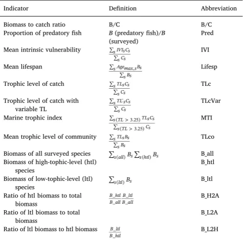
In this study, we included the IndiSeas indicators explored inShin et al. (2018), including biomass to fisheries catch ratio (B/C), propor-tion of predatory fish (Pred), mean intrinsic vulnerability (IVI), mean lifespan (Lifesp), mean trophic level of the community (TLco), and marine trophic index (MTI). In addition, we also explored a range of other indicators, which were either provided in the output of the ten ecosystem models or derived from the outputs of the ecosystem models. These additional indicators included: the trophic level (TL) of catch calculated assuming a constant TL for taxa (TLc) and the TL of catch calculated assuming a variable TL for taxa (TLcVar) (Reed et al., 2017), as well as the biomass of all-trophic-level taxa (B_all), the biomass of HTL taxa (B_htl), the biomass of LTL taxa (B_ltl), the ratio of B_htl to B_all (B_H2A), the ratio of B_ltl to B_all (B_L2A), and the ratio of B_ltl to B_htl (B_L2H) (Table 1). Biomass indicators were identified as Fish Es-sential Ocean Variables by the GOOS (Global Ocean Observing System) Biology and Ecosystems Panel, and have been collected by many ob-serving programmes in the world (Miloslavich et al., 2018).

2.5. Analytical approaches

We employed a machine learning approach to analyze the suite of indicators. Specifically, we used the gradient forest method (R package gradientForest, available online at http://gradientforest.r-forge.r-project.org/) to explore the responses of ecological indicators to changes in fishing pressure and primary productivity alone or in com-bination. The gradient forest method builds upon random forests and thus has all the functionalities of random forests (Ellis et al., 2012).

Random forests are essentially regression tree techniques that do

Fig. 1.Location of the ten marine ecosystems studied (BS = Black Sea, GoG = Gulf of Gabes, NS = North Sea, SCS = Southern Catalan Sea, SEA = Southeastern Australia, SB = Southern Benguela, WC = West coast of Canada, WS = Western Scotland, WFS = West Florida Shelf, and WSS = Western Scotian Shelf). Four ecosystem modelling frameworks were used to simulate the dynamics of these ten ecosystems: Ecopath with Ecosim (EwE), OSMOSE, Atlantis, and multispecies size-spectrum model (SS).

not pre-specify relationships between the response and predictors but rather construct a set of decision rules to recursively partition the data into successively smaller groups with binary splits based on a single predictor variablex(Breiman 2001). Within a regression tree, a split values (which divides the data into two groups with the left group having responses corresponding to predictor values ≤sand the right group having responses corresponding to predictor value > s) is chosen such that it leads to the smallest total impurity, which is the sum of squared deviations about the group mean. The first splits of the regression tree is usually close to the value of the threshold, to which the response is particularly sensitive and beyond which response values shift to another level. Eventually, the recursive partitioning results in a tree that contains branches at the splits and nodes with the mean sponse. At each node, the importance of a split is indicated by the re-duction in impurity in the node induced by the split, measuring the amount of variation that has been explained by the partitioning. Therefore, the split values and their importance contain essential in-formation for revealing the relationships between response and pre-dictors.

While a single regression tree produces output that may be specific to the unique data set, bootstrapping (i.e., resampling with replace-ment) can be used to create similar data sets for constructing multiple trees. When a bootstrap resample is drawn, about one-third of the data (termed “out-of-bag”, OOB) is excluded from the sample, but other data (termed “in-bag”) are replicated to form a full-size sample. Essentially, a random forest consists of an ensemble of trees and each tree recur-sively partitions the data corresponding to the selected split points along the gradient of a predictor. In addition, random forests construct each tree using a randomized subset of predictor variables, thus di-minishing potential effects of correlations among predictor variables. The performance of random forests has been compared with that of other classification/regression tree methods and generally favored in terms of prediction on test data and various other criteria (e.g.Prasad et al., 2006; Cutler et al., 2007; Peters et al., 2007; Knudby et al. 2010).

The gradient forest method integrates individual random forest analyses over the different response variables to capture complex lationships between potentially correlated predictors and multiple re-sponse variables (Ellis et al., 2012). The OOB observations are not used in constructing the trees, thus they provide a cross-validated estimate of the expected variance of the residuals for new observations. The goodness-of-fit measure for the forest for response variabley(R_y2_{) can}

then be obtained by comparing this variance with the variance of the observations:

=

Ry 1 (Y Y ) (Y Y)

i

yi yi

i

yi y

2 2 2

whereYyi is theithobservation of response variabley,Yyi is the OOB

prediction, andYy is the overall mean for response variabley.Ry2

re-presents the proportion of variance explained by the random forest. Each random forest also estimates the importance of each predictor variablex, i.e., accuracy importanceIyx, based on how much worse the prediction would be if the data forxwere permuted randomly.Ry2can

be partitioned into contributions from each predictor variablexin proportion to the accuracy importance, i.e.,

=

R R I

I

yx y yx

x yx

2 2

which can then be averaged across all response variables to obtain the overall importance of the predictor variablex(Rx2). The importance value of a splitsalong the predictor variablexwith respect to response variable y (Iyxs) are aggregated from every tree in the forest and a

density curve is estimated by kernel density estimation. The density curve is then normalized to make the area under the curve equal to the overall importance (Rx2) of the predictor. Upward steep parts of the density curve of split importance values indicate ranges of the predictor where the response variable changes (Ellis et al., 2012). The importance values of splits are standardized by the density and accumulated (cu-mulative importance) along the gradient of predictor to allow the predictor to be assessed in terms of it influence on the response vari-able.

For each of the 14 ecological indicators considered in this study, we ran the gradient forests 1000 times to obtain a range of possibleRy2

values; the run with the highest overall performance (with the highest R2_{) was then used to indicate the performance of the indicators and to} deriveIyx and other statistics. The goodness-of-fit for fishing and for changes in primary productivity expresses thespecificityof the indicator to fishing and changes in primary productivity, respectively. The cu-mulative importance for fishing and changes in primary productivity expresses thesensitivityof the indicator to fishing and changes in pri-mary productivity, respectively. Thresholds along the fishing pressure where ecological indicators vary significantly are defined as the peak values on the normalized density curve where the ratio of the density of split importance to the density of observed predictor values is greater than one.

3. Results

3.1. Overall indicator responses

Overall, the goodness-of-fit of the indicators for fishing (RF2) was

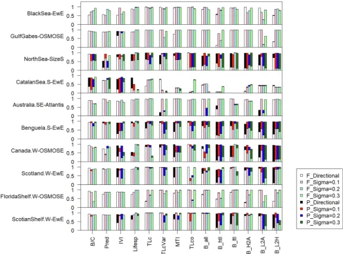
high to very high for seven out of the ten study ecosystems, indicating that the indicators considered in this study were generally capable of tracking changes in fishing levels. With the exception of the North Sea, West Coast Canada, and Southern Catalan Sea, the modelled ecosystems hadRF2close to or greater than 0.9 for most of the ecological indicators,

indicating that the variabilities in these indicators were very well ex-plained by changes in fishing levels (Fig. 2, left panel). This was par-ticularly true for low variability in primary productivity (σ= 0.1). In the West Florida Shelf and Gulf of Gabes,R_F2_{values of most indicators}

under random primary productivity change of σ= 0.3 were equally

Table 1

List of indicators explored. High-trophic-level and low-trophic-level taxa for all the ecosystems are listed inAppendix Table A1. B: biomass (tons); C: catch (tons); s: species; TL: trophic level; TL': variable TL; IVI: intrinsic vulnerability index.

Indicator Definition Abbreviation Biomass to catch ratio B/C B/C Proportion of predatory fish B(predatory fish)/B

(surveyed) Pred Mean intrinsic vulnerability s IVIsCs

s Cs

IVI

Mean lifespan s Agemax sBs s Bs

, Lifesp

Trophic level of catch s TLsCs s Cs

TLc

Trophic level of catch with

variable TL s TL sCss Cs

' _TLcVar

Marine trophic index > >

s TL TLsCs

s TL Cs

( 3.25) ( 3.25)

MTI

Mean trophic level of community s TLsBs s Bs

TLco

Biomass of all surveyed species _{s all}( )Bs s htl( )Bs B_all

Biomass of high-tophic-level (htl)

species B_htl

Biomass of low-tophic-level (ltl)

species s ltl( )Bs B_ltl Ratio of htl biomass to total

biomass B htl B all B ltl B all _ _ _ _ B_H2A

Ratio of ltl biomass to total

biomass B_L2A

Ratio of ltl biomass to htl biomass B ltl B htl

_

high compared to those underσ= 0.1, indicating that these two eco-systems were virtually unaffected by changes in primary productivity. With the exception of the North Sea and, to some extent, the South-eastern Australia, the aggregated biomass indicators B_all, B_ltl, and to some extent B_htl, had generally the lowest RF2 values under both

random and directional changes in primary productivity, indicating that the impacts of fishing were usually least reflected by the ag-gregated biomass indicators. Compared to B_all, B_ltl and B_htl, the biomass ratios (B_H2A, B_L2A, and B_L2H) better reflected the impacts of changes in fishing levels in most ecosystems. With respect to the Southern Catalan Sea, theRF2values of all indicators except Lifesp, TLc,

TLcVar, and MTI were lower than 0.4 under both random and direc-tional changes in primary productivity. This suggested that in the Southern Catalan Sea ecosystem, most of the 14 indicators did not re-flect well the impacts of changes in fishing levels.

With respect to the goodness-of-fit for changes in primary pro-ductivity (RP2), the Black Sea, West Florida Shelf, Gulf of Gabes, and

Southeastern Australia had nearly zero values for all indicators (except for MTI and B_all in the Southeastern Australia, as well as B_all and B_ltl in the Gulf of Gabes), implying that most of the indicators in these four ecosystems did not reflect changes in primary productivity (Fig. 2, right panel). On the other hand, in the North Sea, West Coast Canada, Southern Benguela, Western Scotland, and Western Scotian Shelf, theRP2

values were high for some indicators, particularly biomass-based in-dicators, suggesting that changes of primary productivity in these five

ecosystems could explain variabilities in these indicators. In contrast with all other ecosystems, the Southern Catalan Sea exhibited highRP2

under directional primary productivity change for all indicators other than Lifesp, TLc, TLcVar, and MTI, implying that the dynamics of the Southern Catalan Sea ecosystem was primarily driven by changes in primary productivity when these changes were directional. On the other hand, when there was random variability in primary productivity, changes in primary productivity were no longer able to explain the variations in the indicators.

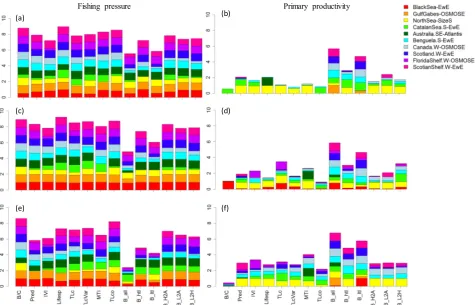
RelativeRF2values (defined as the ratio of medianRF2of a particular

indicator to the highest medianRF2in an ecosystem) were summed over

all ecosystems to show the specificity to fishing pressure of a specific indicator across all ecosystems (Fig. 3a, c, e). The summed relativeR_F2

values were highest for indicators B/C and Lifesp under both directional (Fig. 3a) and random primary productivity change ofσ= 0.1 (Fig. 3c). In addition, relativeRF2values summed over all ecosystems were higher

for B/C and TLco than for other indicators under random primary productivity change ofσ= 0.3 (Fig. 3e). This suggests broad utility of these three indicators (B/C, Lifesp, TLco) for evaluating fishing impacts. In contrast, the three aggregated biomass indicators (B_all, B_ltl, and to some degree B_htl) always resulted in the lowest sum of relativeRF2

values, suggesting inadequacy of these indicators for evaluating fishing impacts. In contrast with the aggregated biomass indicators, the bio-mass ratios (B_H2A, B_L2A, and B_L2H) were relatively better indicators for fishing impacts.

Fig. 2.Stacked bar plots of model performance (goodness-of-fitR2_{) of the gradient forests for each of the 14 study indicators in the ten marine ecosystems when (1)} using fishing mortality as the predictor variable under four different scenarios of primary productivity (F_Directional, F_Sigma = 0.1, F_Sigma = 0.2, and F_Sigma = 0.3), and (2) using primary productivity as the predictor variable under the four primary productivity scenarios (P_Directional, P_Sigma = 0.1, P_Sigma = 0.2, and P_Sigma = 0.3). Ecological indicator abbreviations are listed inTable 1.

Similarly, relativeRP2values (defined as the ratio of medianRP2of a

particular indicator to the highest median RP2 in an ecosystem) were

summed over all ecosystems to show the specificity to primary pro-ductivity variability of a specific indicator across all ecosystems (Fig. 3b, d, f). Overall, the indicators tended to be more responsive to changes in primary productivity when the changes in primary pro-ductivity were characterized by a high variability (σ= 0.3). Under all three primary productivity scenarios, most indicators were less re-sponsive to changes in primary productivity than they were to changes in fishing pressure. Exceptions were the aggregated biomass indicators, B_all and B_ltl, which always resulted in the highest sum of relativeRP2

values, suggesting the utility of these indicators for evaluating the im-pacts of primary productivity change.

3.2. Sensitivity in indicator responses

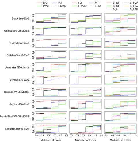
We contrasted the sensitivity of indicators to fishing and primary productivity, by looking at indicators' response to directional change in fishing pressure and to directional change in primary productivity se-parately. For all ecosystems except the Black Sea, the Southern Catalan Sea and, to some extent, the Southeastern Australia, the cumulative importance shifts (inRF2unit) of the indicator B/C in response to fishing

pressure were high even under the lowest fishing levels (Fig. 4, first column). This implied that the B/C indicator was extremely sensitive to fishing pressure. The indicator Lifesp also responded to relatively low fishing pressure in half of the ecosystems (i.e., the Gulf of Gabes, Southern Catalan Sea, West Coast Canada, Western Scotian Shelf, and West Florida Shelf). In contrast, the indicator IVI was not sensitive to changes in fishing pressure in three ecosystems (i.e., the West Coast Canada, West Florida Shelf, and Western Scotian Shelf). Similarly, the indicator Pred was not sensitive to fishing pressure in the Southern

Catalan Sea, West Coast Canada and Western Scotland. In response to directional change in primary productivity, all the indicators were in-sensitive in all ecosystems except the North Sea and Southern Catalan Sea (Appendix Fig. A1, first column).

Among the four TL-based indicators, TLco tended to respond to low fishing levels in all ecosystems except the Southern Catalan Sea, West Coast Canada, and West Florida Shelf, where MTI was the indicator that responded to low fishing levels (Fig. 4, second column). TLcVar re-sponded to lower fishing pressure than TLc in five ecosystems (i.e., the Gulf of Gabes, the North Sea, West Coast Canada, West Florida Shelf, and Western Scotian Shelf). With regard to changes in primary pro-ductivity, these four TL-based indicators were essentially unresponsive in all ecosystems except the North Sea and Southern Catalan Sea (Appendix Fig. A1, second column).

In half of the ecosystems (the Gulf of Gabes, West Coast Canada, West Florida Shelf, Western Scotland, and Western Scotian Shelf), B_htl responded to low fishing pressure around 0.6*FMSY (Fig. 4, third column), indicating that even low fishing pressure can trigger drastic changes in B_htl in these five ecosystems. In all ecosystems except the Gulf of Gabes and Southern Benguela, B_L2A did not show any re-sponses to fishing pressure until the fishing mortality rate of exploited taxa reached the level of 0.8*FMSY. This implied that the indicator B_L2A was not sensitive to changes in fishing pressure when fishing levels were relatively low. In contrast with other indicators, the six biomass-based indicators tended to show greater responses to changes in primary productivity in all ecosystems except the Black Sea, South-eastern Australia, and West Florida Shelf (Appendix Fig. A1, third column), confirming that biomass-based indicators were sensitive to changes in primary productivity and less responsive to fishing pressure.

(a) (b)

) d ( )

c (

) f ( )

e (

y ti v it c u d o r p y r a m ir P e

r u s s e r p g n i h si F

3.3. Thresholds along fishing pressure

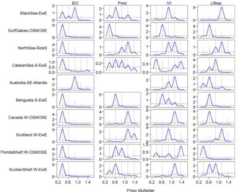
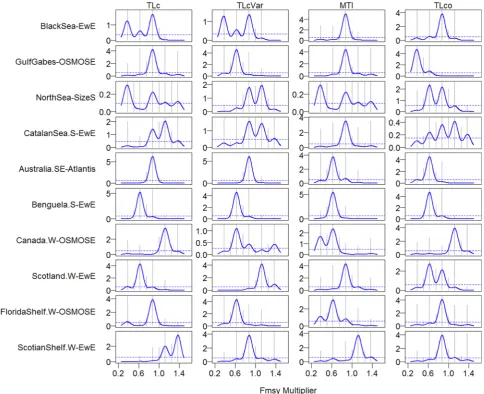
Comparing the density plots from the scenario of fishing pressure with directional change in primary productivity (Figs. 5–7) with those of fishing pressure with random changes in primary productivity (Appendix Figs. A2–7), we found great similarities in terms of thresh-olds in indicators' response to fishing pressure. This indicated that the thresholds identified through the gradient forest method were robust to environmental variability and change. Below we used the scenario of directional change in primary productivity for demonstration purposes. The global result across all indicators and ecosystems revealed that around 44% of threshold responses occurred at fishing pressure values

within 0.9–1.1*FMSY. Considering thresholds of individual indicators across all the ecosystems, the density curves of the indicator B/C showed the most consistent unimodal peaks (Fig. 5). Other indicators showed unimodal peaks in nearly half of the ecosystems (Figs. 5–7), indicating monotonic changes in the indicators as fishing monotonically increased. When indicators had more than one peak, the dominant peak showed coherence across at least half the ecosystems, such as Pred and Lifesp (Fig. 5) and B_all, B_H2A, B_L2A (Fig. 7). Compared to B/C that had thresholds around 0.4*FMSYalong the gradients of fishing pressure in eight of the ten ecosystems, all other indicators tended to have higher threshold fishing levels around 0.6–0.9*FMSYin most of the ecosystems. Among the biomass-based indicators, B_L2H tended to have higher

Fig. 4.Cumulative importance along the gradient of fishing levels (multiplier ofFMSY) in ten marine ecosystems with first column for indicators B/C (biomass to fisheries catch ratio), Pred (proportion of predatory fish), IVI (mean intrinsic vulnerability), and Lifesp (mean life span); second column for TLc (mean trophic level TL of catch), TLcVar (mean TL of catch with variable TL), MTI (marine trophic index), and TLco (mean TL of fish community surveyed); and third column for B_all (biomass of all species), B_htl (biomass of high-trophic-level species), B_all (biomass of low-trophic-level species), B_H2A (the ratio of B_htl to B_all), B_L2A (the ratio of B_ltl to B_all), and B_L2H (the ratio of B_ltl to B_htl).

thresholds in some ecosystems such as Western Scotland and Western Scotian Shelf (Fig. 7).

Within ecosystems, threshold responses across indicators ranged from around 0.3 to 1.4*FMSY (Figs. 5–7). Interestingly, the Southern Benguela ecosystem manifested a consistent level of threshold around 0.6*FMSYfor all indicators except B/C that had a lower threshold value. In the Southeastern Australia and West Florida Shelf ecosystems, half of the indicators had thresholds around 0.6*FMSYwhile about another half of the indicators had thresholds around 0.8–0.9*FMSY. In the Black Sea, nine indicators showed thresholds round 0.8–0.9*FMSY, while in West Coast Canada, more than half of the indicators displayed even higher threshold values around 1.1*FMSY. In contrast, the western Scotian Shelf had one indicator (B/C) around 0.4*FMSY, three indicators with thresholds around 0.6*FMSY, six indicators showed thresholds around 0.8–0.9*FMSY, and four indicators had threshold values greater than 1.0*FMSY.The Catalan Sea frequently had multiple peaks (greater than2) in the indicator response curves.

4. Discussion

Identifying and applying a suite of ecological indicators that are responsive to fishing pressure, capable of tracking changes in the state

of marine ecosystems, and related to management objectives are ne-cessary for moving toward EBFM. Due to the complex nature of marine ecosystems that are subject to multiple anthropogenic and environ-mental stressors, there is a critical need to assess the specificity and sensitivity of indicators to fishing (Houle et al., 2012; Hunsicker et al., 2016; Shin et al., 2018; Otto et al., 2018). In this study, using a multi-ecosystem, multi-model simulation experimentation design and the gradient forest approach for analyzing model and scenario outputs, we have obtained insights into the specificity and sensitivity of 14 key indicators to changes in fishing pressure and primary productivity. In particular, the similarity in indicators’ performance across the ten ecosystems provides a solid foundation for the selection of indicators and their applications in fisheries management.

4.1. Comparison with previous work

Using the signal-to-noise-ratio approach,Shin et al. (2018) identi-fied the indicators that were relatively more specific to fishing than to changes in primary productivity. By adopting the gradient forest method in this study, we were able to draw conclusions on the amount of variability in each indicator that was explained specifically by fishing or by changes in primary productivity, which provided all indicators

with a unique property of specificity not only to fishing but also to changes in primary productivity. Most importantly, the gradient forest method enables us to move beyond the evaluation of indicators’ spe-cificity to assess indicators’sensitivity to both fishing pressure and changes in primary productivity. This advancement has great implica-tions for EBFM; indicators that respond to low fishing levels are fun-damentally essential for EBFM and therefore deserve more attention both in terms of research and monitoring. Most importantly, the gra-dient forest analyses have provided us with threshold levels along the gradients of fishing pressure for all the indicators across the ecosystems, the application of which could substantially support decision-making in EBFM.

Although we only explored indicator response under the “all-trophic-levels” fishing strategy, we conclusively showed that B/C was the indicator with the highest specificity to fishing; the indicators Lifesp and TLco were also found to have higher specificity compared to other indicators (Fig. 3), consistent withShin et al. (2018). In addition, both studies concluded that when variability in primary productivity in-creased, indicators tended to be less specific to fishing, which highlights the need to identify indicators that are robust to noise in the environ-ment when evaluating fishing impacts.

Compared to studies based on empirical data (e.g.Large et al., 2015;

Tam et al., 2017), our simulation study achieved much higher good-ness-of-fit for fishingRF2 with seven out of ten ecosystems havingRF2

close to or greater than 0.9 for most of the ecological indicators. This is due to the fact that historical (observed) fishing levels in a specific exploited ecosystem varied over time, whereas the same relative fishing level was implemented consistently across all model simulation years under the controlled simulation experimentation, resulting in much predictable consequences from fishing impacts. Nevertheless, our model simulation experimentation revealed the indicators’ relative specificity and sensitivity to changes in fishing and primary pro-ductivity.

4.2. Ecosystem-specific responses

Our results also confirm those ofShin et al. (2018), who concluded that the performance of indicators was influenced by the signatures of individual ecosystems. As such, evaluations of indicator performance need to consider the ecosystem history and fishing context. For ex-ample, in the Southern Catalan Sea, which has a long fishing history and where current fishing mortality rates are very high, all indicators, with the exception of Lifesp, TLc, TLcVar and MTI, hadR_F2_{values lower}

than 0.4, and even lower under random changes in primary

Fig. 6.Threshold shifts in the values of four trophic level (TL) based indicators (TLc: mean TL of catch, TLcVar: mean TL of catch with variable TL, MTI: marine trophic index, and TLco: mean TL of fish community surveyed) along the gradient of fishing pressure under directional change in primary productivity. The dashed line indicates where the ratio of the density of split importance to the density of observed fishing pressure is 1; peaks above the dashed line suggest threshold values for the fishing pressure.

productivity characterized by a small variability (σ= 0.1). In contrast, Lifesp, TLc, TLcVar and MTI had highRP2for the Southern Catalan Sea

under the directional change in primary productivity (Fig. 2), in-dicating that the Southern Catalan Sea food web was under “bottom-up control” after a long history of fishing exploitation. Essentially, these results suggest that when the whole ecosystem has been fished down, these indicators are no longer very responsive to changes in fishing levels but were primarily driven by directional change in primary productivity, as has been previously highlighted (Shannon et al., 2014; Coll et al., 2016; Lockerbie et al., 2017a). In the North Sea,RP2values

were exceptionally high yetRF2values were the lowest for all indicators

except B/C, TLco, and B_ltl under random change in primary pro-ductivity withσ= 0.3. This may be caused by the fact that one parti-cularly abundant fish species in the North Sea ecosystem (plaice, Pleuronectes platessa) has a high growth rate and feeds on macro-invertebrate which respond strongly to changes in primary production, thus drastically reducing the specificity and sensitivity to fishing under large random changes in primary productivity. Similarly, in the West Coast Canada ecosystem, the high variability of indicators’ specificity and sensitivity, as well as the highRP2values for most indicators,

par-ticularly the biomass-based indicators, could be explained by the changes in the biomass of the most abundant LTL species of the eco-system, Pacific herring (Clupea pallasii). All in all, the above-mentioned ecosystem-specific responses of indicators to different stressors high-light the need for involving local experts in indicator studies, which is a key tenet of the IndiSeas programme (Shin et al., 2012, 2018).

4.3. Directional and random changes in primary productivity

For most indicators in most ecosystems, theRF2values under

direc-tional change in primary productivity were lower than those under random changes in primary productivity (Fig. 2). This implies that in the presence of directional environmental change, the variability of

indicators could be explained by both fishing and directional environ-mental changes. However, with the rather narrow range of directional change (with a multiplier between 0.85 and 1.1) in primary pro-ductivity,RP2values were generally low. In particular, these values were

near zero in four ecosystems (the Black Sea, Gulf of Gabes, Southeastern Australia, and West Florida Shelf), indicating that nearly all the in-dicators were unresponsive to small directional changes in primary productivity. However, additional simulations exploring primary pro-ductivity change are warranted in order to verify the preliminary conclusions drawn from this study.

In the situation of indicators’ responses to fishing pressure under random changes in primary productivity, theRF2 values for most

in-dicators in most ecosystems tended to be the highest (largely above 0.8) under small random variability (i.e.,σ= 0.1), implying that the gra-dient forest method had the ability to capture the impacts of fishing when the variability of environmental changes was low (σ= 0.1). However, as environmental variability increased (i.e., whenσwas set to 0.3), theRF2values declined in most ecosystems. This is an important

result for researchers and fisheries managers, as there would likely be increasing variability in primary productivity in the future resulting from global climate change (Winder and Cloern, 2010), such as in the Southern Benguela where variability in upwelling indices increased in the 1990 s and 2000 s presumably because of climate change (Blamey et al., 2012). Nevertheless, our framework (Fig. 2) provides the po-tential to identify indicators that would be more robust to increasing noise in the environment of a specific ecosystem (e.g.,RF2underσ= 0.3

is equally high as or close to that underσ= 0.1), or to tease out in-dicators that tend to have drastically lowerRF2underσ= 0.3 than that

underσ= 0.1. We found that the indicator B/C had equally highRF2

values under all environmental scenarios across all ecosystems except the Southeastern Australia and the Southern Benguela, suggesting that the B/C indicator was generally robust in detecting fishing changes even in the presence of large environmental noise. In contrast, the

aggregated biomass indicators (B_all, B_htl, and B_ltl) appeared to have consistently high sensitivity to environmental noise across most eco-systems, indicating the inadequacy of these indicators for detecting fishing impacts. This particular result is important, as it has not been uncommon to employ aggregated biomass indicators for examining fishing impacts in the past (e.g. Fu et al., 2012; Coll et al., 2016; Miloslavich et al., 2018).

4.4. Sensitivity of indicators

Among the 14 indicators, B/C was found to have the highest sen-sitivity to fishing pressure, followed by Lifesp, TLco, and B_htl. These indicators responded sharply to fishing from a threshold of around 0.6* FMSYor lower in most ecosystems (Fig. 4). Previous work has shown that some component-specific indicators, such as biomass of gadoids, biomass of clupeids, and the pelagic to demersal biomass ratio were sensitive to different fishing and environmental stressors (e.g.Fu et al., 2012; Large et al., 2015; Tam et al., 2017). Here we showed that, in contrast with all other indicators, only the six biomass indicators were found to be sensitive to changes in primary productivity. The compar-ison of the sensitivities of the two indicator groups (six biomass in-dicators and all the others) in response to either fishing or changes in primary productivity suggested that all indicators other than the bio-mass indicators were performing better if only the evaluation of fishing impacts was of concern. However, the biomass indicators would be important for assessing the impacts of changes in primary productivity. The need for multiple suites of indicators to capture ecosystem impacts from multiple stressors was supported by a number of other studies (e.g. Blanchard et al., 2014; Link et al., 2010; Fu et al., 2012, 2015). This result add nuance to the results ofLarge et al. (2015), who concluded that ecological indicators were more responsive to anthropogenic pressures than to environmental pressures.

4.5. Thresholds and reference points

This work adds to the growing body of knowledge on ecosystem threshold response and provides direction for potential reference points for fisheries management. Overall, there was some degree of con-sistency in threshold response across indicators and ecosystems sug-gesting their potential utility for EBFM. Notably, over 50% of the 14 indicators explored had threshold responses at, or below ∼0.6* FMSY for most of the ten ecosystems, indicating that in these modelled eco-systems most indicators would have already crossed a threshold when fished atFMSY. This adds a clear ecosystem perspective to EBFM and, with an exploration of the ecosystem impacts of crossing this threshold, enables informed decisions to be made on what is an acceptable eco-system change, or an acceptable cost of fishing.

The consistent threshold response in the indicator B/C at low levels of fishing pressure (around 0.4*FMSY) suggested that this indicator

would be a good candidate for assisting in ecosystem-level decision making for fisheries management across the globe, although B/C is unlikely to be responsive at higher levels of fishing pressure. However, most other indicators had variable threshold responses across the dif-ferent study ecosystems, implying that the investigation of threshold fishing levels, the implications of crossing the threshold and their translation into reference points, need to be operationalized on an ecosystem-to-ecosystem basis, as has been promoted in other indicator-based studies such as those relying on the decision tree framework (Lockerbie et al., 2016, 2017a,b).

Ideally, a suite of indicators for EBFM would include indicators with complimentary threshold responses at different levels of pressure, thus enabling a portfolio approach to assessing and managing for ecosystem change. With the exception of the Southern Benguela and Gulf of Gabes, the threshold responses of the indicators explored here included threshold values near the lower and upper limits of the fishing pressure range considered, thus forming the basis of a potential suite of

indicators.

In terms of ecosystem functioning, with the exception of the Catalan Sea, there was a relative consistency of thresholds across indicators for a given ecosystem. This suggests that in the all-species fishing situation, all facets of biodiversity and ecosystem status represented by the di-versity of indicators are affected concomitantly with potentially large impacts from a specific threshold of fishing level.

4.6. Advantages, uncertainties and future work

The multi-ecosystem, multi-model approach proved to be valuable for conducting a cross-comparison of indicators’ specificity and sensi-tivity and identifying robust responses of indicators to stressors. The cross-comparison was made possible by using standardized designs of changes in fishing pressure and primary productivity across ecosystems and models. Although differences in model structure (e.g. phyto-plankton forcing, differential emphasis on ecological processes) and the different species and taxa represented in the different ecosystem models could influence simulation outcomes (Heath et al., 2013), there were no clear differences in indicator specificity and sensitivity among the four different types of modelling approaches. The different responses and sensitivities of indicators to fishing and changes in primary productivity were more likely to be influenced by ecosystem structure (e.g. the species/taxa composition of a given ecosystem) and, to a larger extent, by fishery exploitation history. We would, however, caution that having a suite of models would be more helpful to quantify uncertainties due to model structure and modelled processes, as well as to tease out actual differences of indicators' response across regions due to specific eco-system features and exploitation history. Nevertheless, we conclude that the gradient forest method combined with a multi-ecosystem, multi-model approach is a powerful way to assess and compare the performance of ecological indicators despite the potential uncertainties in model and ecosystem structures mentioned above.

We envision different research avenues regarding ecological in-dicators. First, we could employ a similar approach as that used in the present study to determine indicators' responses and thresholds under other fishing strategies than the one considered in this study (fishing across all trophic levels), e.g. when fishing focuses on either high- or low-trophic-level taxa. These additional analyses would enable us to also examine indicator performance in light of the fishing strategy adopted in a marine ecosystem (Shin et al., 2018). Second, concerning environmental variability, due to the constraints imposed by our comparative modelling approach, we had to rely on a proxy that was a common forcing variable to the various ecosystem models used in our study, thus we simplified the simulations by generating directional and random changes in primary productivity. Depending on the ecosystem modelling approach employed, future simulations using a set of re-levant environmental drivers (e.g. water temperature, salinity, oxygen concentration, mixed layer depth) could be carried out to more realis-tically reflect the impacts of environmental change on ecosystem dy-namics and functioning.

Third, while the 14 indicators considered in the present study are intended to track changes in ecosystem attributes, such as biodiversity and resilience, they are expected to be responsive to changes in fishing pressure over a relatively short time scale to be useful for EBFM. Therefore, we recommend the responsiveness (i.e., time of response) of indicators be explored in future studies as part of the performance evaluation process. Finally, the thresholds identified here can be con-sidered a preliminary investigation into tipping points, that is points beyond which the ecosystems may be subject to irreversible changes (e.g.Moore, 2018). Future work could benefit from identifying non-linear ecosystem responses to multiple stressors and detecting tipping points, which would help managers set non-arbitrary targets to avoid detrimental ecosystem shift and maximize social and economic return (e.g.Foley et al., 2015).

5. Conclusions

By applying the gradient forest methodology, we were able to draw conclusions on indicators' specificity not only to fishing but also to changes in primary productivity. It was concluded that the performance of biomass indicators for evaluating fishing impacts was low, but was high and better suited for assessing the impacts of changes in primary productivity on ecosystem status. The indicator B/C was identified as having the highest sensitivity to fishing, as well as the ability to mea-sure fishing impacts at very low levels of fishing presmea-sure. Furthermore, B/C is a simple indicator to calculate and is, therefore, an excellent candidate for immediate future research to make this a valuable in-dicator for fisheries managers and EBFM. Overall, the fishing thresholds at which indicators responded rapidly were belowFmsy, and were ro-bust to environmental variability and largely consistent across the dif-ferent indicators we considered within a specific ecosystem. This highlights the great potential of these indicators to be developed further in applied situations to support decision-making in EBFM.

Declaration of Competing Interest

None.

Acknowledgements

We thank the participants of the IndiSeas Working Group for the useful discussions and insights since the early stages of the study. We are very grateful to Penny Johnson for her modelling work on Atlantis, Philippe Verley and Huizhu Liu for the technical support on OSMOSE, and Jeroen Steenbeck for development of EwE simulation routines.

Funding

This is a contribution to the IndiSeas Working Group, co-funded by IOC-UNESCO (www.ioc-unesco.org) and EuroMarine (http:// www.euromarinenetwork.eu), to the project EMIBIOS (FRB, contract no. APP-SCEN-2010-II) and to the IOC-UNESCO GOOS Program and GOOS Biology and Ecosystems Panel. The work on Canada West Coast ecosystem was sponsored by Fisheries & Oceans Canada under the Aquatic Climate Change and Adaptation Services Program. YJS and LV were supported by the project EMIBIOS (FRB, contract no. APP-SCEN-2010-II). AG was supported by NOAA’s Integrated Ecosystem Assessment (IEA) program (http://www.noaa.gov/iea/). LJS was sup-ported by IRD, France, and through the South African Research Chair Initiative, funded through the South African Department of Science and Technology (DST) and administered by the South African National Research Foundation (NRF). JEH was supported by a Beaufort Marine Research Award carried out under the Sea Change Strategy and the Strategy for Science Technology and Innovation (2006-2013), with the support of the Marine Institute, funded under the Marine Research Sub-Programme of the Irish National Development Plan 2007-2013. MC was supported by the Marie Curie Career Integration Grant Fellowships – PCIG10-GA-2011-303534 - to the BIOWEB project. All other authors were supported by their respective affiliations.

Appendix A. Supplementary data

Supplementary data to this article can be found online athttps:// doi.org/10.1016/j.ecolind.2019.05.055.

References

Aberhan, M., Kiessling, W., Fürsich, F.T., 2006. Testing the role of biological interactions in the evolution of mid-Mesozoic marine benthic ecosystems. Paleobiology 32, 259–277.https://doi.org/10.1666/05028.1.

Akoglu, E., 2013. Nonlinear Dynamics of the Black Sea Ecosystem and Its Response to

Anthropogenic and Climate Variations. PhD thesis. Middle East Technical

University.

Alexander, K.A., Heymans, J.J., MaGill, S., Tomczak, M., Holmes, S., Wilding, T.A., 2015. Investigating the recent decline in gadoid stocks in the west of Scotland shelf

eco-system using a food-web model. ICES J. Mar. Sci. 72, 436–449.

Araújo, J.N., Bundy, A., 2011. Description of the ecosystem models of the Bay of Fundy, Western Scotian Shelf and NAFO Division 4X. Canadian Technical Report of Fisheries

and Aquatic Sciences 2952.

Araújo, J.N., Bundy, A., 2012. The relative importance of climate change, exploitation and trophodynamic control in determining ecosystem dynamics on the western

Scotian Shelf, Canada. Mar. Ecol. Prog. Ser. 464, 51–67.

Blamey, L.K., Howard, J.A.E., Agenbag, J., Jarre, A., 2012. Regime-shifts in the southern

Benguela shelf and inshore region. Prog. Oceanogr. 106, 80–95.

Blanchard, J.L., Andersen, K.H., Scott, F., Hintzen, N.T., Piet, G., Jennings, S., 2014. Evaluating targets and trade-offs among fisheries and conservation objectives using a

multispecies size spectrum model. J. Appl. Ecol. 51, 612–622.

Boyce, D.G., Dowd, M., Lewis, M.R., Worm, B., 2014. Estimating global chlorophyll

changes over the past century. Prog. Oceanogr. 122, 163–173.

Breiman, L., 2001. Random forests. Machine Learning 45, 5–32.

Bundy, A., Coll, M., Shannon, L.J., Shin, Y.J., 2012. Global assessments of the status of marine exploited ecosystems and their management: what more is needed? Curr.

Opin. Environ. Sustain. 4 (3), 292–299.

Christensen, V., Walters, C., 2004. Ecopath with Ecosim: methods, capabilities and

lim-itations. Ecol. Model. 72, 109–139.

Coll, M., Palomera, I., Tudela, S., Sardà, F., 2006. Trophic flows, ecosystem structure and fishing impacts in the South Catalan Sea, Northwestern Mediterranean. J. Mar. Syst.

59, 63–96.

Coll, M., Navarro, J., Palomera, I., 2013. Ecological role of the endemic Starry ray Raja asterias in the NW Mediterranean Sea and management options for its conservation.

Biol. Conserv. 157, 108–120.

Coll, M., Shannon, L.J., Kleisner, K.M., et al., 2016. Ecological indicators to capture the effects of fishing on biodiversity and conservation status of exploited marine

eco-systems. Ecol. Indic. 60, 947–962.

Cutler, D.R., Edwards, T.C., Beard Jr., K.H., Cutler, A., Hess, K.T., Gibson, J., Lawler, J.J.,

2007. Random forests for classification in ecology. Ecology 88, 2783–2792.

Ellis, N., Smith, S.J., Pitcher, C.R., 2012. Gradient forests: calculating importance

gra-dients on physical predictors. Ecology 93, 156–168.

Fay, G., Large, S.I., Link, J.S., Gamble, R.J., 2013. Testing systemic fishing responses with

ecosystem indicators. Ecol. Model. 265, 45–55.

Foley, M.M., Martone, R.G., Fox, M.D., Kappel, C.V., Mease, L.A., Erickson, A.L., Halpern, B.S., Selkoe, K.A., Taylor, P., Scarborough, C., 2015. Using Ecological Thresholds to Inform Resource Management: Current Options and Future Possibilities. Front. Mar. Sci. 2, 95.https://doi.org/10.3389/fmars.2015.00095.

Fu, C., Gaichas, S., Link, J.S., Bundy, A., Boldt, J.L., Cook, A.M., Gamble, R., Utne, K.R., Liu, H., Friedland, K.D., 2012. Relative importance of fishing, trophodynamic and environmental drivers in a series of marine ecosystems. Mar. Ecol. Prog. Ser. 459,

169–184.

Fu, C., Perry, R.I., Shin, Y.-J., Schweigert, J., Liu, H., 2013. An ecosystem modelling framework for incorporating climate regime shifts into fisheries management. Prog.

Oceanogr 115, 53–64.

Fu, C., Large, S., Knight, B., Richardson, A., Bundy, A., Reygondeau, G., Boldt, J., et al., 2015. Relationships among fisheries exploitation, environmental conditions, and

ecological indicators across a series of marine ecosystems. J. Mar. Syst. 148, 101–111.

Fu, C., Travers-Trolet, M., Velez, L., et al., 2018. Risky business: the combined effects of fishing and changes in primary productivity on fish communities. Ecol. Model. 368,

265–276.

Fulton, E.A., Parslow, J.S., Smith, A.D., Johnson, C.R., 2004. Biogeochemical marine ecosystem models II: the effect of physiological detail on model performance. Ecol.

Model. 173, 371–406.

Fulton, E.A., Smith, A.D.M., Punt, A.E., 2005. Which ecological indicators can robustly

detect effects of fishing? ICES. J. Mar. Sci. 62, 540–551.

Fulton, E.A., Smith, A.D.M., Smith, D.C., Johnson, P., 2014. An integrated approach is needed for ecosystem based fisheries management: insights from ecosystem-level

management strategy evaluation. PLoS One 9, e84242.

Garcia, S.M., Zerbi, A., Aliaume, C., Do Chi, T., Lasserre, G., 2003. The ecosystem ap-proach to fisheries. FAO Fisheries Technical Paper. N°443. FAO, Rome.

Garcia, S.M., Kolding, J., Rice, J., Rochet, M.-J., Zhou, S., Arimoto, T., Beyer, J.E., Borges, L., Bundy, A., Dunn, D., Fulton, E.A., Hall, M., Heino, M., Law, R., Makino, M., Rijnsdorp, A.D., Simard, F., Smith, A.D.M., 2012. Reconsidering the consequences of

selective fisheries. Science 335, 1045–1047.

Grüss, A., Schirripa, M.J., Chagaris, D., Velez, L., Shin, Y.-J., Verley, P., Oliveros-Ramos, R., et al., 2016. Evaluating natural mortality rates and simulating fishing scenarios for

Gulf of Mexico red grouper (Epinephelus morio) using the ecosystem model

OSMOSE-WFS. J. Mar. Syst. 154, 269–279.

Greenstreet, S.P.R., Rossberg, A.G., Fox, C.J., Le Quesne, W.J.F., Blasdale, T., Boulcott, P., Mitchell, I., Millar, C., Moffat, C.F., 2012. Demersal fish biodiversity: species-level indicators and trends-based targets for the Marine Strategy Framewotk Directive.

ICES J. Mar. Sci. 69, 1789–1801.

Halouani, G., Lasram, F.B.R., Shin, Y.-J., Velez, L., Verley, P., Hattab, T., Oliveros-Ramos, R., et al., 2016. Modelling food web structure using an end-to-end approach in the

coastal ecosystem of the Gulf of Gabes (Tunisia). Ecol. Model. 339, 45–57.

Heath, M.R., Speirs, D.C., Steele, J.H., 2013. Understanding patterns and processes in

models of trophic cascades. Ecol. Lett. 17, 101–114.

Heymans, J.J., Coll, M., Libralato, S., Morissette, L., Christensen, V., 2014. Global pat-terns in ecological indicators of marine food webs: a modelling approach. PLoS One

Heymans, J. J. and Tomczak, M. T., 2016. Regime shifts in the Northern Benguela eco-system: challenges for management. In: Ecopath 30 years - Modelling ecosystem dynamics: beyond boundaries with EwE. Ecol. Model. 331, 151–159.

Houle, J.E., Farnsworth, K.D., Rossberg, A.G., Reid, D.G., 2012. Assessing the sensitivity and specificity of fish community indicators to management action. Can. J. Fish.

Aquat. Sci. 69, 1065–1079.

Hunsicker, M.E., Kappel, C.V., Selkoe, K.A., Halpern, B.S., Scarborough, C., Mease, L., Amrhein, A., 2016. Characterizing driver–response relationships in marine pelagic

ecosystems for improved ocean management. Ecol. Appl. 26, 651–663.

Kershner, J., Samhouri, J.F., James, C.A., Levin, P.S., 2011. Selecting indicator portfolios

for marine species and food webs: A Puget Sound case study. PLoS ONE 6, e25248.

Knudby, A., Brenning, A., LeDrew, E., 2010. New approaches to modelling fish–habitat

relationships. Ecol. Model. 221, 503–511.

Large, S.I., Fay, G., Friedland, K.D., Link, J.S., 2015. Critical points in ecosystem re-sponses to fishing and environmental pressures. Mar. Ecol. Prog. Ser. 521, 1–17.

https://doi.org/10.3354/meps11165.

Link, J.S., Yemane, D., Shannon, L.J., Coll, M., Shin, Y.-J., Hill, L., Borges, M.F., 2010. Relating marine ecosystem indicators to fishing and environmental drivers: an

elu-cidation of contrasting responses. ICES J. Mar. Sci. 67, 787–795.

Link, J.S., Gaichas, S., Miller, T.J., Essington, T., Bundy, A., Boldt, J., Drinkwater, K.F., Moksness, E., 2012. Synthesizing lessons learned from comparing fisheries produc-tion in 13 northern hemisphere ecosystems: emergent fundamental features. Mar.

Ecol. Prog. Ser. 459, 293–302.

Lockerbie, E., Shannon, L.J., Jarre, A., 2016. The Use of Ecological, Fishing and Environmental Indicators in Support of Decision Making in Southern Benguela

Fisheries. Ecol. Model. 69, 473–487.

Lockerbie, E., Coll, M., Shannon, L.J., Jarre, A., 2017a. The use of indicators for decision

support in northwestern Mediterranean Sea fisheries. J. Mar. Syst. 174, 64–77.

Lockerbie, E.M., Lynam, C.P., Shannon, L.J., Jarre, A., 2017b. Applying a decision tree framework in support of an ecosystem approach to fisheries: IndiSeas indicators in

the North Sea. ICES J. Mar. Sci. 75 (3), 1009–1020.

Miloslavich, P., Bax, N.J., Simmons, S.E., Klein, E., Appeltans, W., Aburto-Oropeza, O., Andersen, G.M., Batten, S.D., 2018. Essential ocean variables for global sustained observations of biodiversity and ecosystem changes. Glob. Chang. Biol. 24, 2416–2433.https://doi.org/10.1111/gcb.14108.

Möllmann, C., Diekmann, R., MÜLler-Karulis, B., Kornilovs, G., Plikshs, M., Axe, P., 2009. Reorganization of a large marine ecosystem due to atmospheric and anthropogenic pressure: a discontinuous regime shift in the Central Baltic Sea. Glob. Chang. Biol. 15, 1377–1393.https://doi.org/10.1111/j.1365-2486.2008.01814.x.

Moore, J.C., 2018. Predicting tipping points in complex environmental systems. Proc.

Natl. Acad. Sci. USA 115, 635–636.

Otto, S.A., Kadin, M., Casini, M., Torres, M.A., Blenckner, T., 2018. A quantitative

fra-mework for selecting and validating food web indicators. Ecol. Indic. 84, 619–631.

Peters, J., Baets, B., Verhoest, N., Samson, R., Degroeve, S., Becker, P., Huybrechts, W., 2007. Random forests as a tool for ecohydrological distribution modelling. Ecol.

Model. 207, 304–318.

Piet, G.J., Hintzen, N.T., 2012. Indicators of fishing pressure and seafloor integrity. ICES

J. Mar. Sci. 69, 1850–1858.

Prasad, A.M., Iverson, L.R., Liaw, A., 2006. Newer classification and regression tree techniques: Bagging and random forests for ecological prediction. Ecosystems 9,

181–199.

Probst, W.N., Kloppmann, M., Kraus, G., 2013. Indicator-based status assessment of commercial fish species in the North Sea according to the EU Marine Strategy

Framework Directive (MSFD). ICES J. Mar. Sci. 70, 694–706.

Reed, J., Shannon, L., Velez, L., Akoglu, E., Bundy, A., Coll, M., Fu, C., Fulton, E.A., Grüss,

A., Halouani, G., Heymans, J.J., Houle, J.E., John, E., Le Loc'h, F., Salihoglu, B., Verley, P., Shin, Y.J., 2017. Ecosystem indicators – accounting for variability in

species' trophic level. ICES J. Mar. Sci. 74, 158–169.

Rice, J.C., Rochet, M.-J., 2005. A framework for selecting a suite of indicators for fisheries

management. ICES J. Mar. Sci. 62, 516–527.

Samhouri, J.F., Andrews, K., Fay, G., Harvey, C.J., Hazen, E.L., Hennessy, S.M., Holsman, K., Hunsicker, M.E., Large, S.I., Marshall, K.N., Stier, A.C., Tam, J.C., Zador, S.G., 2017. Defining ecosystem thresholds for human activities and environmental pres-sures in the California Current. Ecosphere 8, e01860.https://doi.org/10.1002/ecs2.

1860.

Shannon, L.J., Christensen, V., Walters, C., 2004. Modelling stock dynamics in the southern Benguela ecosystem for the period 1978–2002. Afr. J. Mar. Sci. 26,

179–196.

Shannon, L.J., Neira, S., Taylor, M., 2008. Comparing internal and external drivers in the southern Benguela and the southern and northern Humboldt upwelling ecosystems.

Afr. J. Mar. Sci. 30, 63–84.

Shannon, L.J., Coll, M., Bundy, A., Gascuel, D., Heymans, J.J., Kleisner, K., Lynam, C.P., et al., 2014. Trophic level-based indicators to track fishing impacts across marine

ecosystems. Mar. Ecol. Prog. Ser. 512, 115–140.

Shin, Y.-J., Cury, P., 2001. Exploring fish community dynamics through size-dependent trophic interactions using a spatialized individual-based model. Aquat. Living Resour.

14, 65–80.

Shin, Y.-J., Shannon, L.J., Bundy, A., Coll, M., Aydin, K., Bez, N., Blanchard, J.L., et al., 2010. Using indicators for evaluating, comparing, and communicating the ecological status of exploited marine ecosystems. 2. Setting the scene. ICES J. Mar. Sci. 67,

692–716.

Shin, Y.-J., Bundy, A., Shannon, L.J., Blanchard, J.L., Chuenpagdee, R., Coll, M., Knight, B., Lynam, C., Piet, G., Richardson, A.J., the IndiSeas Working Group, 2012. Global in scope and regionally rich: an IndiSeas workshop helps shape the future of marine

ecosystem indicators. Rev. Fish Biol. Fish. 22, 835–845.

Shin, Y.-J., Houle, J.E., Akoglu, E., Blanchard, J.L., Bundy, A., Coll, M., Demarcq, H., Fu, C., Fulton, E.A., Heymans, J.J., Salihoglu, B., Shannon, L., Sporcic, M., Velez, L., 2018. The specificity of marine ecological indicators to fishing in the face of

en-vironmental change: a multi-model evaluation. Ecol. Indic. 89, 317–326.

Smith, A.D.M., Brown, C.J., Bulman, C.M., Fulton, E.A., Johnson, P., Kaplan, I.C., Lozano-Montes, H., Mackinson, S., Marzloff, M., Shannon, L.J., Shin, Y.-J., Tam, J., 2011. Impacts of fishing low-trophic level species on marine ecosystems. Science 333,

1147–1150.

Stephenson, R.L., Wiber, M., Paul, S., Angel, E., Benson, A., Charles, A., Chouinard, O., Clemens, M., Edwards, D., Foley, P., Lane, D., McIsaac, J., Neis, B., Parlee, C., Pinkerton, E., Saunders, M., Squires, K., Sumaila, R., 2018. Integrating diverse ob-jectives for sustainable fisheries in Canada. Can. J. Fish. Aquat. Sci Can.https://doi.

org/10.1139/cjfas-2017-0345.

Tam, J.C., Link, J.S., Large, S.I., Andrews, K., Friedland, K.D., Gove, J., Hazen, E., Holsman, K., Karnauskas, M., Samhouri, J.F., Shuford, R., Tomilieri, N., Zador, S., 2017. Comparing apples to oranges: common trends and thresholds in anthropogenic and environmental pressures across multiple marine ecosystems. Front. Mar. Sci. 4,

282.https://doi.org/10.3389/fmars.2017.00282.

Travers, M., Shin, Y.-J., Shannon, L.J., Cury, P., 2006. Simulating and testing the sensi-tivity of ecosystem-based indicators to fishing in the southern Benguela ecosystem.

Can. J. Fish. Aquat. Sci. 63, 943–956.

Winder, M., Cloern, J.E., 2010. The annual cycles of phytoplankton biomass. Phil. Trans.

R. Soc. B 365, 3215–3226.

Zhou, S., Smith, A.D.M., Knudsen, E., 2015. Ending overfishing while catching more fish.

Fish Fish. 16, 716–722.