Performance analysis of self-organized Ad-Hoc sensor networks

Rochester Institute of Technology

RIT Scholar Works

Theses

Thesis/Dissertation Collections

2004

Performance analysis of self-organized Ad-Hoc

sensor networks

Venkateswararao Oruganti

Follow this and additional works at:

http://scholarworks.rit.edu/theses

This Thesis is brought to you for free and open access by the Thesis/Dissertation Collections at RIT Scholar Works. It has been accepted for inclusion in Theses by an authorized administrator of RIT Scholar Works. For more information, please [email protected].

Recommended Citation

Performance

Analysis

of

Self-organized

Ad

hoc Sensor Networks

By

Venkateswararao

Oruganti

Thesis

submitted

in

partial

fulfillment

ofthe requirements

for

the

degree

of

Master

of

Science in Information

Technology

Rochester

Institute

of

Technology

B. Thomas Golisano College

of

Computing

and

Information

Sciences

Rochester Institute of Technology

B. Thomas Golisano College

of

Computing and Information Sciences

Master of Science in Information Technology

Thesis Approval Form

Student Name: Venkateswararao Oruganti

Thesis Title: Performance Analysis of self Organizing Ad-Hoc Sensor

Networks

Thesis Committee

Name

Signature

Date

Prof Fei Hu

Fei Hu

D2-//p/Dr

Chair

Prof Luther Troell

Luther Troell

~

j(,1o~

Committee Member

Prof Nirmala Sheno~

Nirmala Shenoy

62-!r

i

/05

Thesis Reproduction Permission Form

Rochester Institute of Technology

B. Thomas Golisano College

of

Computing and Information Sciences

Master of Science in Information Technology

Performance Analysis of self Organizing Ad-Hoc

Sensor Networks

I, Venkateswara Oruganti, hereby grant permission to the Wallace Library of the

Rochester Institute of Technology to reproduce my thesis in whole or in part.

Any reproduction must not be for commercial use or profit.

Performance

Analysis

of

Self-organized

Ad

hoc Sensor Networks

Presented by: Venkat Oruganti

Advisor: Dr. Fei Hu

Committeemembers: Prof LutherTroell& Prof Nirmala

Shenoy

This project deals with a Distributed Sensor Network (DSN). The main focus ofthis

thesis is to deliveran OPNET simulation model for _{working DSN} model. After

building

a _model, various performance analysis techniques in terms ofdifferentparameters were

used to_verifythe _working model.

Query

Dominant Sets

(QDS)

arethemain idea behind

this thesis. The QDS node is incharge ofthe nodes fora specific region andits job is to

assign the _query tasks that it getsto the nodes in that region to

help

maximizethe life of

the network. Ifno user queries are

being

_{sent, the} QDS nodesthemselves go to _sleep to

conserve _energy andjust listen for special

incoming

control signals. QDS management

(including

the selection ofQDS and the interaction of QDS nodes and other common

nodes) is a_challengingissue in DSNplatforms.

Our algorithm for QDS management attempts tolimit the dead spots in the network that

tend to disrupt the communication ofthe whole network. It has two phases and the first

phase is the election phase. The second stage is the _previously elected QDS nodes

distributethe tasks to theother nodes. Thisalgorithmturns out tobe distributed which is

good for sensor networks. There is no use of_any global communication or

long-range,

high energydata communication, butjust local communications. Thisalso helps tosave

power and _energy for

long

life ofthe sensors. This algorithm is also _very scalable and

faulttolerant.

We have done significant simulations to _verify our QDS concepts. There are some

metricsthatare usedtoevaluate our schemes such as the average _energyvalues of all the

nodes in the network, minimum _energy of all the nodes in the network, total _energy

consumedin the awake, transmit, andreceive _states,maximumtime spent

by

_anynodein

electing a new

QDS,

number ofelected

QDSs,

and so on. Our simulations have shown

Acknowledgements

It is _gratifying to be able toput _many

long

days andtheoretical _{understanding} to complete this thesis.

Making

the project a _reality takes _many simple steps from the

beginning

to the end and it is _my pleasure to thank and acknowledge everyone involved intheprocess.

First of _all, I would like to thank Prof. Fei

Hu,

thesis advisor for advising,

motivating and _reviewing the work from time to time. Hehas been a great motivator all the while from the time I met him in summer 2002 while

taking

Wireless Networks course in Computer

Engineering

department. He defined the research goals and set out the path for me to navigate through the complex world ofresearch. I thank him for his

advice, recommendations andmotivationthroughout thisperiod.

I would like to thank Prof. Luther Troell for _agreeing to be on the panel of committee members. I still remember how amazingly he explained the architecture of

Internet in one of _my graduate classes. I also thank Prof Nirmala

Shenoy

for _readily

agreeing to be a committee member and

being

supportive. I appreciate and thank their gracious_{understanding} andhelpfulnature.

It was _challenging to get this project _rolling and _stay on track since it went through a lotoftwists and turns. I thankHarsha and Sreenivas for their valuable

help

in

troubleshooting

and

debugging

problems while in lab. Iwish themsuccess and good luck intheirfuture endeavors.

Finally

I want to thank _my friends and office colleagues who have been patient and supportive while I was _grumpy at times due to stress developed in

balancing

school and work.

Lastly

I would like to thank _my

family

for

inspiring

and _{encouraging in}

9

IV

Contents

Acknowledgements

TableofContents

ListofFigures

Introduction i

1.1 Sensor Network ₂

1.2 Sensor Network_{considerations}

4

1.3 Network Architecture Issues 5

1.4 Thesisorganization ₇

Relatedresearch anddevelopmentwork ₉

2.1 Sensor Nodes ₉

2.2

Routing

andNode communication 12

2.3 DataAggregation ₁₃

3

Query

Dominant Sets

(QDS)

₁₅

3.1 Selection issues 15

3.2 Algorithmfor_selectingMaximal independent Set 16

3.3 CommunicationMethods. 21

3.3.1 Singlepath_routingwithrepair 22

3.3.2 Optimal Path Setup: 23

4 Test Scenariosand results ₂₉

4. 1 Simulationtools ₂₉

4.2 Node andProcess Models ₃₃

4.3 Testcase Scenario 34

4.4 _{Results Analysis 35}

5 Conclusion ₄₂

List

of

Figures

Fig

1.1 Example of a sensor network

Fig

2. 1 WINSwireless sensor node

Fig

2.2 uAmpsWireless sensorNode (sizecomparison with a_penny)

Fig

2.3 PicoRadio Project Sensor Node

Fig

3.1 Maximal IndependentSetofNodes

Fig

3.2

Query

DominantSet Node Selection

Fig

3.3 Optimal Path BlockDiagram.

Fig

3.4 Flowdiagram for

determining

abrokenlink

Fig

3.1

Primary Hierarchy

ofOPNET Models

Fig

4.2 Processsteps ofdataextraction and result generation

Fig

4.3 TheNodemodel of a sensor node

Fig

4.4 SelectionofQDS ina regular sensor network.

Fig

4.5 Parameters for simulation

Fig

4.6 MaximumTime spent on_electingQDS (forparameters

fig 4.5)

Fig

4.7 Anotherset ofparameters

Fig

4.8 MaximumTimespent on _{electing QDS}(forparameters

fig

4.7)

Fig

4.9 Global Powerofthenetwork

Fig

4.10Taskcount,

Asleep

timeandPoweranalysisI

Fig

4.1 1 Taskcount.

Asleep

timeandPoweranalysisII

1.

Introduction

A sensoris defined as a device thatreceives and responds to a signal or stimulus

and in turn _may or _may not send another signal as a responseto it. Ingeneral it is a

tiny

electromagnetic device that receives and transmits different radio waves. A sensor

network isan autonomous _groupof

tiny

sensorsthataredistributedover an area such as a

farm

land, battlefield,

_{ocean, parking lots etc. The recent advances in hardware and}

software communications technologies have let manufacturers make a large number of

sensors with wide capabilities in a cost effective manner. Different features of a sensor

node are as follows

a)Small in size

-Inrecent

days,

sensor nodes are _slightlybiggerthana quarter

b)

Inexpensive

-Nodes canbemanufactured fora couple of cents each.

c) Unattended

-Nodesare_usuallyused_onlyonce and are unattended.

d)

Limitedresources

-Nodes have less computingpower, low_memoryandlow

energythatcan sustain for onlyafew daysorhours

depending

on power

utilization.

As a whole, the sensor nodes are _unreliable, have

low-energy

and do not have _many

capabilities. But we desire to forma robust, long-lived sensor network out of such short

lived,

unreliable sensor nodes. This _may sound unusual but a good set of node

distribution _methods, robust data

forwarding

techniques and reliable communication

scenarios comprised together can make a more efficient sensor network. The _only

problem here would be that this network would never be as reliable as a TCP/IP or

there can be a lessreliable butuseful network insuch areas as

battlefield,

forests or _any

such environmentswhere it isnexttoimpossibletoinstalladatanetwork.

1.1.

Sensor

Network

As _previously mentioned a sensor network is an autonomous _group of sensor

nodes or _sensing devices deployed in a region. The sensor nodes have processing and

wireless capabilitiesthatenableittogatherinformationfromtheenvironmentand sendit

to a remote base station. In our _thesis, a sensor network consists of the

following

constituents.

a) Sensornodes

b)

Query

Dominant Set

(QDS)

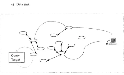
node(also calledclusterheadorleadnode)

c) Data sink

Fig

-1.1 Exampleofasensornetwork

The sensor nodes above shown are typical ones as described earlier. The QDS

(Query

[image:11.538.59.477.328.582.2]

as described in thelater chapters. Thedata sinkis _normallyadata center place which has

a ground network _running from it. A data sink can be on the ground or in a over

flying

airplane. But the data sink is usually connected to outside world. The data is collected

from the QDS _nodes, analyzed and converted to a form thatmakes sense to the outside

world. Therecan bethousands of sensor nodes andhundreds ofQDS nodesand a couple

ofdatasinks inalarge sensor network.

Atypicaldistributedsensor networktransfers data betweendifferentnodes. Butin

our _case, the nodes transfer signals or data to the QDS nodes

thereby

_saving a lot of

energy

by

not _sending powerful _energy driven data signals to the sink themselves. The

QDS node collects information from the normal nodes andsends itto the sink. The QDS

nodes also can send their information to the other QDS node ifthe data sink is too far

from it.

The above diagram(Fig- 1.1

)

is a scenarioof a sensornetwork. There iscouple of

nodes, some QDSnodes andadatasink. Thepurpose oftheabovenetwork istoillustrate

a_working sensornetwork. Imaginetheabovesensor networkinaforest. _{The query} target

is to find out ifthere is a fire in that particular area ofthe network. When the target is

fixed,

a data signal comes from the data sink to the QDS node which in turn sends a

signal to that area node. The nearby node gets activated and the traces for _any carbon

monoxide orcarbon dioxide inthe targetedarea. Ifittraces or_not, it sends a signal to the

an _easy task. But there are a lot ofaspects involved in the signal transfer. Some of the

considerationsaboutsensornodes,QDSnodes, datasink are asfollows

1.2.

Sensor Network

_{considerations}

There are some major considerations for the components involved in a sensor

network.

First,

it is the sensor node. The size, power and _capacity ofthe node are some

factorspertained toit. When

distributed,

they

shouldbevisible and need tobeinthe level

view oftheQDS node sothat the communicationbetweenthem isnotinterfered. Itis not

possible at all times tohave such ahospitable environment. Ifthe sensor networkis

being

deployed in a dense forest or a

battlefield,

then there is a high _possibility of nodes

becoming

dead or useless due to various factors. When it comes _{to power,} it is

directly

proportionalto the size ofthenode. The smallerthe size ofthe node,the lowerthepower

of it

thereby

_{making it} more vulnerable to become useless after some usage. When the

node's power is exhausted it is discarded. The only way to replenish the nodes is to

distribute some morenodesinthenode depletedarea.

Other consideration is the communication between the nodes. Sensor nodes

cannot be wired for several reasons.

So,

the sensor networks are constructed with a

wireless topology. The data sink though, is connected to the outside world _mostly

by

a

The other consideration is the protocols used in the construction of a wireless

network. Conventional protocols cannot be used since

they

require a lot of energy. New

protocols are required todeliveradequate _{coverage,availability} and _energyconservation. There should be a lot of _{redundancy built into} the network in order to have reliable

coverage even when nodesbecome useless more often.

1.3

Network Architecture

Issues

Distributed Sensor Networks are in a _way a new set of networks that work

independently

irrespective of their environment unlike traditional wire line ad-hoc networks or infrastructure-basedwireless networks. Someofthe

key

characteristics are

a)

Mobility

-Ifthenodes arenotstatic itbringsconsiderable challenges interms of

topology

changes andnetworklogic. Thewireless sensor networks canbeequippedwith

specialhardwarethatmakes themmobilewhichinturncreates some challenges. This

thesis doesn'taddressthe_mobilityofnodechanges.We assume a static sensor network

b)

Routing

(single

hop

or Multi

hop)

redundant protocol that keeps the network alive for a longer time and helps insure a

reliabledatatransfer.

c) Medium

-traditional networks use wire medium to transfer signals. But in a

wireless sensor _{network, the} medium is radio waves. Radio waves are susceptible to

interference and fading. Packet loss is another major problem in radio wave

communications. For example a simulation _study

[1]

of a 50 node ad-hoc network

distributedover a 1500 x300 m area shows that therewere 1 1,857 link failures

during

a

900 second simulation period when each node moved at a speed of0 - 20

m/s. Though

we do not consider mobile nodes, the error rate is _pretty high when compared to

traditionalwireline networks.

d)

Routing

-Traditional routing protocols are designed

taking

into consideration of

unlimited power _supplywhich is not the same in a wireless sensor network. We have to

use protocols that do not form loops or send the same information to the same recipient

node again and again.

Also,

theoverhead to control networktraffic mustbe low so as to

ensure _energy conservation in the nodes. The routing protocols should converge at a

faster speed when

topology

changes occur

thereby

_ensuring an accurate and low cost

route.

There are some other issues like fault tolerance, environment and infrastructure

issues that also need to be addressed. In general, a wireless sensor network has all the

1.4

Thesis

organization

The main focus of this thesis is to deliver an OPNET simulation model for _working sensor

network model. After

building

a model, various performance analysis techniques in terms of

differentparameters were used to_verifythe _working model. Itdeals with a distributed sensor

network.

Query

Dominant Sets

(QDS)

arethemainidea behind this thesis. The firstpart

dealswithhow toselect aQDS node

by

a mathematical model. The second partdescribes

how a QS node assignsthe tasks to thenodes

by

_getting a_query fromthe Sink. TheQDS

node is incharge ofthe nodes for a specific region andits job is toassignthe _query tasks

that itgets to the nodesin thatregionto

help

maximizethe lifeofthenetwork. Thenode

mustbe able to coverthe entire region, either

by

itselforthrough theuse of other nodes.

If a node is not needed for any particular or elongated _{time, it} can be put to _sleep to

conserve

battery

power. Ifnouser queries are

being

_{sent, the} QDS nodes themselves go

to _sleeptoconserve_energyandjust listen for special

incoming

control signals.

This thesis is organized in the

following

manner. The firstpart is an introduction

to wireless sensor networks, its characteristics and issues. Different aspects of sensor

networks

including

various constraints, challenges and features are discussed with

emphasisto_energyconservation andsimple _routingalgorithms.

The second part gives an overview of _ongoing research and development of

network architectures that were proposed and implemented in the last few years are

discussed.

The third part explains a mathematical approach to determine a maximal

independentsetfrom Luby's Monte Carlomethod. A QDS

(Query

Dominant

Set)

node is

determined withthis process which acts as a clusterhead. An approach to communicate

with the sensor network is also explained. This approach tries to _prolong the life ofthe

sensor network

by

_{utilizing redundancy in}nodestocreateload balanceandreliablesignal

transfer. The concept of single-path and multi-path _routing techniques are discussed.

Althoughwe donot use or prove _anything,we assume single path scenariointhe thesis.

The fourth part introduces metrics and simulation results. An introduction to

OPNET and the simulation parameters are discussed. The results are analyzed and

presented _alongobservedtrends inthe simulations done. There are some metrics that are

used to evaluate our ideas such as the average _energy values of all the nodes in the

network, minimum _energy ofall the nodes in the network, total energy consumed in the

awake, transmit, and receive states, maximum time spent

by

_any node in _electing a new

QDS,

number of elected

QDSs,

and so on.

The conclusion discusses possiblefuture workthatcanbe done starting fromthis

thesis. We also discuss the deficiencies in the proposed system andchallenges that need

2.

Related

research and

development

work

Thework on normalsensors began

long

before last decadeand evolvedovertime.

Sensors were used in automobiles and other industries in a _very specific way. These

sensors were small and did a _very few tasks.

They

were connected to one processor

which receives signals from the sensors and then processed. These sensors had no

processing capability or_anymemory and

they

were usedjust forspecifictasks. With the

advent oflow cost computers to the user end,

technology

evolved in bothhardware and

software. This ledto the creation of alotofdevices thatare smallin sizebut performeda

lotoftasks. Hardware advancements made all electronic devices small andthis ledto the

creation of anew set of sensors thatareinexpensive.

2.1.

Sensor

Nodes

The first_{known working} sensor network wasdeveloped

by

UCLA. In the project

named WINS (Wireless Integrated Network

Sensors) [10]

at UCLA and

Rockwell,

a

sensornetwork was developedthat integrated_{sensing, processing} and communication on

micro-sensor platforms [11]. These sensors were fabricated _using low-power wireless

integrated micro-sensor

technology (LWIM)

and are capableof

forming

self-assembling,

multi-hop networks [4]. The transmission ofdata in these sensors was done through the

radio-frequencymodem built intothe sensor. These sensors were made _using lowpower

wireless integrated microprocessor technology. Their main applications are in _seismic,

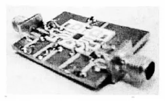
Fig

2.1 WINS wireless sensor node

The Smart Dust project

[14]

was completed in

2001,

but it has led to other

projects. One

interesting

thing

about the Smart Dust project is the small size of the

sensors. These sensors were based on MEMS based

technology

[15].

They

are under a

fewmillimetersinsize and store no morethan 1 Joule of_energywithpowerconsumption

in the microwatt levels. These nodes are also capable of a range of_upto a few hundred

meters and a datatransferrate ofkilobits persecond. Auser can communicate withthese

nodes _using a mobile base station with a transceiverunit. This research analysis proved

that communication in a range offew hundred meters is possible at several kilobits per

second.

The micro-Adaptive Multi-domain Power-aware Sensors

(uAmps)

project is a

project at the Massachusetts Institute of Technology. uAmps project also looks into

power conservation at the software level. This is an all inclusive project as it included

designing

the nodes, software, and protocols forcommunicationbetween thenodes. The

nodes were designed tobe power-aware.

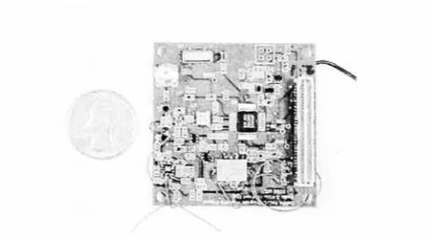
Fig

2.1 is a sensor node inthe uAmps project.

The softwarewritten and theprotocols designed forthese nodes made it veryeffective to

prolong the life of the node. Another aspect of this project is the _{data processing}

[image:19.538.199.369.52.163.2]

algorithms that resulted in two common signal _processing applications namely, finite

impulse

response

filtering

andimage decoding.

[16,

13]

i~m.

\L

ff"\

Fig- _{2.2 uAmps Wireless sensorNode (sizecomparisonwitha}

penny)

The PicoRadio Project

[12]

is aproject ofthe

Berkeley

Wireless Research Center

that involved

developing

the PicoRadiowireless sensor node. ThegoalofthePicoRadio

project was to

"Develop

meso-scale low cost (< _{50 cents)} transceivers for ubiquitous

wireless data acquisition that minimizes _power/energy

dissipation"

An

interesting

fact

about thesewirelessnodes is that

they

arepoweredthroughsolar energy. [image:20.538.140.376.134.267.2] [image:20.538.149.350.456.603.2]

These are some of the major technological places where research on wireless sensor

networks is

being

done. Rockwell Science

Center,

Crossbow

Inc,

ZigBee Alliance and

many other public and privatecompanies are also_pursuingand

developing

them.

2.2

Routing

and

Node

communication

Energy

conservation is the main issue thatneeds tobe factored in

developing

_any

routing protocol or communication techniques. The _energy consumption level is

dependentontheprotocol stack used innode communication.

So,

theprotocol hasto slim

and also robust enough to give a reliable communication and data transfer. Several

protocols have been proposed and _variety of power _saving techniques has been

introduced. Someoftheprotocols include

LEACH, SPIN,

DSDVetc.

LEACH (Low

Energy

Adaptive

Clustering Hierarchy)

is designed for sensor

networks where an end-user wants to _remotely monitor the environment. In such a

situation, the data fromthe individual nodes mustbe sentto a central base station, often

located far from the sensor network, through which the end-user can access the data.

Conventional network protocols, such as direct _{transmission,} minimum transmission

energy, _multi-hop routing, and _clustering all have drawbacks that don't allow them to

achieve all the desirable properties. LEACH includes distributed cluster

formation,

local

processing to reduce global communication, and randomized rotation of the

cluster-heads.

Together,

these features allow LEACH to achieve the desired properties. Initial

simulations show that LEACH is an energy-efficient protocol that extends system

lifetime.

SPIN is a

family

of protocols used to _efficiently disseminate information in a

wireless sensor network. _{Conventional data dissemination} approaches like

flooding

and

gossiping waste valuable communication and _energy resources _sending redundant

information throughout the network. _{In addition,} these protocols are not resource-aware

or resource-adaptive. SPIN solves these shortcomings of conventional approaches _using

data negotiation and resource-adaptive algorithms. Nodes running SPIN assign a

high-levelnameto their

data,

called_meta-data,and perform meta-data negotiations before any

data is transmitted. This assures that there is no redundant data sent throughout the

network. _{In addition, SPIN}has accessto the current _{energy level} ofthenode and adapts

the protocolitis running basedon howmuch _{energy isremaining}

Basic

Energy

Conservation Algorithm

(BECA)

and Adaptive

Fidelity Energy

Conservation Algorithm

(AFECA)

are two _routing algorithms introduced

by

Estrin

[8]

that _{introduce sleep} mode to the nodes when

they

are not needed.

They

also use node

density

to let _neighboring nodes to handle traffic in case of less power scenarios. The

PicoRadio research addresses network layer

by introducing

designs for the MAC layer

using dynamic channel assignment techniques.

Multi-hop

_routing and multiple channel

communications are thecharacteristics intheirproposal.

2.3

Data

Aggregation

Once the _routing techniques are

finalized,

the sensor network _efficiency lays in

one final and importantissue i.e. dataaggregation and interpretation. All signals are sent

to the

Query

Dominant Set nodes and

they

inturn forward itto the sink. There arc _many

factorstobe consideredin

doing

this.

The raw data or theinformal signals that are sent

by

the nodes to the QDS nodes

maynotbeas efficient as the user wants ittobe. And eveniftheinformation is efficient,

the cost of_sending the complete data that it got to the sink might be too expensive and

drain all the _energy resources ofthe QDS node.

So,

the QDS node must segregate the

important inforation and then _relay itto the sink. Another factor isthe _possibility of one

QDS node_solving the entire_query itself.

Many

queries _{may involve} multiple QDS nodes

which inturn assign multipletasks to thenodes.Data aggregationis an importantissue to

be considered while _proposing a wireless sensor network. This topic is mentioned here

but is out ofreach for this thesis. We assume that the communication between the sink

andtheQDSnodes isthrough a solid reliablenetwork. Thisthesis dealswiththe network

and transportlayers but not thedata link or application layer if discussed inconventional

networks.

3.

Query

Dominant

Sets

(QDS)

The sensor nodes are _{normally distributed randomly} over an area with no set of

rules or design. When the sensor nodes are

distributed,

all of them are assumed to be

having

same _energy level and capabilities. After the

distribution,

the first _step in our

wireless network is

determining

the_querydominantset node.

3.1

Selection issues

A QDS node is a node in the network that receives and transmits signals to the

sink, designates itself as the sensor head _among a couple of _neighboring sensors and

assigns tasks to the adjacent sensor nodes. A QDS node selection is based on different

factors

including

power level of _{the node, workload,} number oftasks and _adjacency to

various other nodes. In general it is a node that manages a set of nodes in a particular

region.

The primary purpose ofthe QDS node is to increase the networklife as much as

possible

by

_assigning and _resolving queries in a power _saving and reliable way. The

sensing coverage of aQDS node is similarto the others. So ithastouse the _neighboring

nodes _sensingcapabilities while

tasking

and _answeringa query. This requires that it is in

proximityofallthenodesin itsregion.

Energy

saving is the most important goal of_any node. This cannot be achieved

unless nodes are switched off when

they

are not

being

used. The QDS node is in charge

of sending a signal to _sleep off to its regional nodes. The QDS node also can go to

hibernation mode if

they

are not

being

used. This whole power scheme depends on the

kind of _sensing coverage needed from the sensor network. A network in a battlefield

requires the nodes to be active most of the time since there is a high availability

requirement for such kind of networks. Consider a wireless sensor network in a

deep

forest that _{has been deployed for counting endangered species like} tigers. The network

doesn't need to be available all the time and most ofthe nodes can go to _sleep mode

during

certain periods. The power scheme can be decided and programmed into the

sensors before

they

arc deployed or canbe put to _sleep

by

the QDS node.

Reliability

of

the network is equally important and proper care need to be taken while

deciding

to get

balance betweenpower scheme and reliability.

The QDS selection can e explainedin two parts. The firstpart explains sequential

algorithm to find a Maximal Independent Set for simple graphs. This algorithm can be

modified and used in distributed networks. The simple algorithm selects all independent

nodes and ifmodified

by

_adding some constraints in sensor networks will work to find

the QDS nodes in a distributed network. The second part describes how the Luby's

MonteCarloalgorithm

[6]

of_{selecting Maximal Independent} sets inadistributedpattern.

3.2

Algorithm

for

selecting

Maximal

independent Set

The first_step istodescribe theselectionof a maximal independentsetin alinear

graph. The sensornetwork isrepresentedinasimplelineargraph. The basic algorithm

formaximal independentsetisdeterminedas follows.

Assume the network

by

a linear graph G =

(V, E). Each vertex

V,

represents a

sensor node in the network and E is Edge set

{E(Vj

,

V,

)}

that represents two adjacent

nodes. The neighbor is determined

by

the _ability ofthe radio ofnode i toreach the radio

ofthenodej. A maximal _independentset isan independentset SofG ifall the vertices of

G are cither in S or adjacent to a vertex in S where G is a subsetofV such that no two

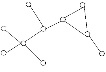
vertices ofS areadjacent_{in G [7]. This}canbe betterexplainedinadiagram.

Fig

3.1 Maximal Independent SetofNodes

The nodes that are red are selected as the Maximal independent set

by

the above

conditions. The above sequential algorithm can _{be mathematically} put like this. A set

Nc(I)

is defined to be a neighbor set ofI in G. Ateach iteration a vertex is chosen from

the setV anddetermined if it belongs to the _{group NG(I). If it}is not inthe _groupthenit is

added to theIndependentset I.

For all v V

do

If v i

NG(I)

then

I = _{I U v}

End if

End

do

Since the sensor network is distributed we need to determine the maximal

independent

set in a parallel _{way among} all the nodes. The Luby's algorithm has to be

improved

to [image:26.538.130.315.187.314.2]

work in a distributed environment. Jones andPlassman

[3]

developed a methodwhich is

used as abasis forour sensornetwork.

The maximal independent set nodes aredetermined in a _way that does not _really

fulfill ourrequirement forselection of a

Query

Dominant Sets. Sowe need tomake some

improvements to get the needed set of nodes. Luby's Monte Carlo algorithm lets us

determine a minimum number of nodes fromthemaximalindependent set. Thiswas used

by

Jones and plassman

[3]

to create a method for vertex _coloringa graph in parallel. In

this method, the initial independent setI ' is determinedwhich make_up

Nc (

I ') Thenext

step involvesremoving ofUnion of sets I 'and

Nq (

I'

)

fromV ' _{The remaining} vertices

inV 'is thesubset of maximal independentsetthatwe need. Thisis explainedas follows.

While G1 _<>

0

do

Select

an Independent set I ' in

G

'

I = _{I U} I1

H = I1 _U

NG(

I '

)

V ' = V '

\

H

G

' = G(V

')

End

do

Using

this algorithm we deduce a similar algorithm to get an independent

Query

dominant set. This is done

by

_selecting a set of

Query

Dominant set nodes such that a

node i is aQDS node ortheeffective radio coverage ofthatsensor node i intersects with

the radio coverageofthe QDS node. Ateach

iteration,

the set of nodesV withneighbors

higherthan their

neighbors'

random numbersis chosen fromthe _remaininggraphH. This

set V is addedto the maximal independent setandthen subtracted from H _along withthe

nodesthatare neighbors ofH. S is setof nodes andV isthe set of nodes Sthat

belong

to

H = _G

V = _S

While

r

(i)

> r

(j)

While S <>

₀

do

P = _P

\

_V

P = _P

\

adjoining

(V)

I = I U V

H is the graph

induced

by

P

End while End

While

This algorithm chooses an independent set of nodes that are designated as

Query

Dominant Sets. _{It may} be a bit confusingwhile

discussing

distributedsensor nodes in the

terminology

ofset theory.

So,

the nodes

theory

is explained

taking

into consideration a

set of nodes.

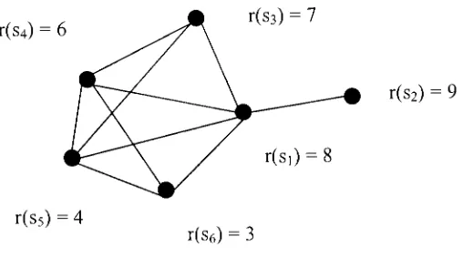
We consider a set of nodes

Sj

where i >0 and I < 7. That gives us a total of six

nodes. Letrbe arandom numberorvalue. Hereweassignarandom numberto the nodes.

The nodes do not need to have _any global communication. The communication is just

between the _neighboring nodes and thus will be _very effective in terms of power. The

first step ofthealgorithmrequiresall_neighboringnodes communicate _{their r(si)}values to

each other. The whole selection process can be explained

by Fig

3.2 in a _step wise

manner as follows.

a) The first step involves as said before communication between

neighboring nodes oftheir random values. The _neighboring nodes are

defined as the nodes that can communicatewith each other i.e. nodes

that have theirradio

frequency

ofnode i intersects with the

frequency

of nodej. In theabove example that factoris _alreadydetermined and is

denoted intheform oflinks betweennodes.

b)

The second _step node s2 elects itselfas a part ofQDS or a QDS node

since its random value is greater than Si. Then it communicates about

its decisionto thenode Si

c) In the third _step s\ broadcasts a message

declaring

its intent not to

become a leader node or QDS node since it _{already knew} about s2

becoming

theQDSnode.

d)

The fourth step node S3 elects itselfas a QDS node since the nodes s4

and S5 have a lesser value. It broadcasts itself as a QDS node even

thoughits random valueis lessthan si because it has heardthe message

from S]

intending

nottobecomeaQDSnode.

e) The fifth step involves nodes S4 and S5

declaring

their intent not to

becomeaQDS node.

They

drop

outbecauseofthesamereason as

they

alreadyheard fromnode S3aboutit

becoming

aQDS node.

f)

In the last _step node sr,declares itselfas aQDS node because it heard

from all the other _neighboring nodes about their intention not to

becometheQDS nodes.

r(s4) =

6

Fig

3.2

Query

Dominant Set Node Selection

Thustheprocess selects a

Query

Dominant Setthatincludesnodes

2,

3 and6. Itis a

small examplethatinvolves a small number of nodes. Thisprocedureis followed ina

distributed_way all_alongthesensornetworktoselect a setofQDSnodes. Thedistributed

sensor nodesthus make_upalarge sensor networkwith a

Query

DominantSetofnodes

thatmanagethem.

3.3

Communication Methods.

The data packet is transferred from a source through destination in various ways

depending

on how many copies of data packets are transferred simultaneously. The

protocolscanbe dividedinto

Single Path

Routing

Multipath

Routing

We use _only single path _routing in our case. For single path _routing we have the data

packet transferred as a single _copy through out the nodes, while in multipath _routing

[image:30.538.156.410.68.209.2]

multiple copies of a data packet are sent _{simultaneously} in different paths to the

destination.

Generally

single path_{routing is}more efficientintermsof_energy savedbut if

there is failure in line it will cause the whole transmission ofdata packet tobe stopped.

On the other

hand,

multipath _routing uses a lot of_energy to transfer packets in parallel

linesand hence the_efficiencygoes down butthe transmission is completed. Comparative

to other _sensors, wireless sensors are prone to more failures and therefore there is a

growing awareness inthe research

industry

touse multipath _routingto ensure thedata is

transmitted even though the _efficiency is less. However the problem in _using the

multipath _routing is

determining

the sensor network topologies before transmission of

data,

as the topologies changes _rapidly due to malfunction of some nodes or

environmental physical damage. Another disadvantage of multipath _routing is the more

traffic is generated for one data packet

delivery,

which _may cause network congestion,

which leadstomore

delay

oftransmissionofdatapacket. Withthese differentadvantages

and disadvantages of single and multipath _routing, we discuss few ofthenew initiatives

thatmightworkfor futureresearch.

3.3.1 Single path _routingwith repair

This process involves sending thedata in a single path and_repairing as and when

a break is occurred. Path repair has been introduced in _many wireless networks

depending

in the type of repair andthe path chosen for data transfer. The process is very

simple, the data packet is send in a single path and whenever a break is detected an

alternative path is created and the data is resent through it .One ofthe major problems

with this type ofdata transfer is ifthere is abreakage atthe farthestnode still the whole

data hastobe resentfromthe startfromthe source node.

In this paper, a local pivot-initiated path _repairing approach will be discussed

where in the nodewhich is the successor_{node, immediate} upstreamnode wherethepath

break is in the next node will have the _{responsibility} to find some alternative paths and

send the data. Althoughthe selected alternative path might not be the optimal path but it

will ensurethedatapacket istransferredto the sink and alsothisprocessis moreefficient

than _sending the wholedata from the source nodeinadifferent path. Such_{energy saving}

shouldoutweigh theadditional _energycaused

by

_usinga non-optimal path. Thenext few

pagesdeal withthe transferofdata ina single path and canbeclassified asfollows.

OptimalPath

Setup

Data

Forwarding

Along

theOptimalPath

Detecting

theBroken link

3.3.2

Optimal

Path

Setup:

Inthis process, before data transmission,an optimal path fromeach sensor nodeis

determined,

which canbe attained

by

a low-costset_upprocess

by initiating

fromthe sink

node. So

by

_{choosing any} optimal path for a single_routing process we can describe our

next process, which will be data

forwarding

_along this optimal path. The Data

Forwarding

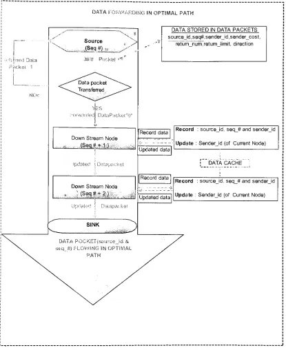
alongtheOptimal Pathis doneas follows.

The data packet is transferred from source node to sink node in a downstream

process, the source

being

the first node and the data packet

being

transferred down the

line _{(downstream) along} the optimal path. The source node is identified

by

a sequence

number

(seq_#)

and as the datapacketis transferred downstreamthe sequence number is

incremented

by

one forthe second node andthe datapacketis forwarded from thatnode

to the third node. The sequence number is incremented at _every node for each new data

packet.

The data packet has the

following

information with it. source

jd,

seq_#,

sender

Jd,

sender

_cost,returnjwm, retumjimit and direction. The data packet is

uniquely identified

by

the combination of a seq_# and source_id.IF the datapacket is

forwardedto a _{downstream successfully it}I s denoted

by

a

binary

value "O'Mfit fails to

send the data packet it is denoted

by

a

binary

value

"1"

The data in the "0" is called as

"forwarding

data path"

and the data stored in "1"

is called _returning data path. Always

thedata in "1"

isreturned to theupstream node. Once thesuccessor node receives a data

packetfrom itsupstreamit hastorecordthe

following

valuesin its datacache, sourcejd,

seq_# and senderJd. Once the data is recorded the data is updated

by

filling

its own

sender_id. Now theupdated datapacketis senttonext node in the downstream as shown

in

fig

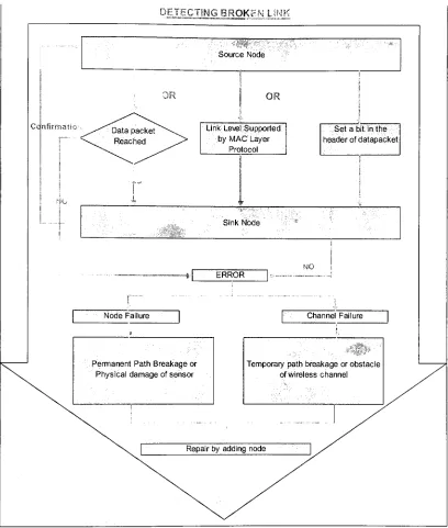
3.3.

3.3.3

Detecting

the

Broken

Link:

The data packet is transferred _along the optimal path which would be decided

before the transfer ofdata packet is started. When a data packet is delivered _along the

lowest cost path, the source node shouldknow any node failure. Toconfirmthat the data

packet has been sent _successfully to the downstream node, it is the _{responsibility} of

successornodeto get a confirmationfromthe _receivingend. This maybe implemented in

one ofthe

following

twoways

(fig

3.4).

DATAFORWARDINGm OPTIMAL PATH

slurriedDala Packet"1"

.:

/

Source (Seg#);

Forwarded DataPackef'O"

Down Stream Node

(Seq#+ 1₎

DATASTORED IN DATAPACKETS

sourceJd,seq#,senderJd,sender_cost,

return num,return limit,direction

Updated Oatauacket

Down Stream Node

, (Seq#+2).

Recorddata

Updated data

Record :sourcejd, seq_# and senderjd

Update: Senderjd (of Current_Node)

DATACACHE

Record data

Updateddata

Record :sourcejd,seq_# and senderjd

Update : Senderjd(of Current_Node)

Fig

3.3 Optimal Path Block Diagram. [image:34.538.64.479.54.562.2]

1. Transmittermonitoring

(passive acknowledgement)

2. Link leveladjustment_{using MAC layerprotocol}

Intransmitter _monitoring a transmittermonitors the packetthatis sent downstream and a

passive acknowledgement is got from the _receiving node as to whether the node was

transmitted _successfullyor not. Ifthelink level is supported

by

MACprotocol layerthen

there isno need forpassiveacknowledgement.If boththesefailthesource_maysend abit

inthe header ofthe data packetto requesttheinformation form each node as towhether

thedatapacket was received or not.

A failederror_maybe becauseofeither ofthesefailures.

Nodefailure

Channel Failure

Node failure refers to permanent path break due to _{energy exhaustion,} malfunction or

physical damage of sensor nodes. Channel error refers to

temporary

path break due to a

collision, interference or obstacle in the wireless channel [2]. Channel errors are

temporary

errors and

they

can be fixed based on the problem. A channel error can be

solved in either

ARQ

or FEC mechanism in data link layer or while in some cases it is

said to be solved in Transport layer. So in ordertoprove that the node needbe replaced

or considered dead and use a redundant path

bypassing

it is the best _way to attend the

problem as an assumption was made that there is no possible layer to repair control

problems. The second assumptionwould

be,

toavoidan extracommunication _overhead;

we don't delve on whether the problem was due to a node failure or channel failure. So

thetransmissionbreak is dealtwith sameway.

DETECTINGBROKEN LINK

SourceNode

OR OR

i>;;";

^^-^Datapacket^\. "*v. Reached fs*

Link LevelSupported byMACLayer

Protocol

Setabit inthe headerofdatapacket

<F '!

Sink Node

NO . 1

ERRO w\

NodeFailure Channel Failure

Permanent Path Breakageor

Physical damageof sensor

Temporarypathbreakageor obstacle of wireless channel

Fig

3.4 Flow diagram for

determining

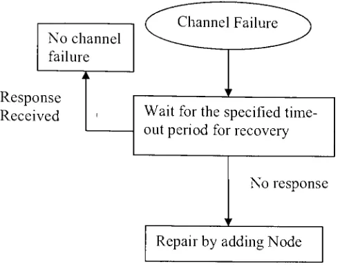
abroken link [image:36.538.65.473.61.542.2]

Nochannel

failure

Response Received

Channel Failure

Wait forthespecifiedtime

out period_{for recovery}

Noresponse

Repair

by

_{adding Node}

Fig

3.5 Flowdiagram for channelfailure

Insome cases, the channel failuremightbejust

temporary

andthelinkmight recoverina

certain time. The other option is to have a certaintime-out period and wait until there is

no response and then confirm the channel failure. As shown in

fig

3.5 when there is a

response received before the time-out _{expires, there} is no need to replace the node o

follow_anyrepairtechnique.

[image:37.538.97.343.109.304.2]

4.

Test Scenarios

and results

The above described algorithms were analyzed and testes with the available

resources. The QDS node selection can be tested in different ways.

By

simple scenario

assumption like the one explained in

fig

3.2 a leader node can be selected. It wastested

with a more complex sensor network and different QDS nodes. If the scope and

complexity of a sensornetworkis

large,

there needtobe several testcases and scenarios

to test theparameters properly. We begintoshowtheresults

by

describing

thesimulation

environmentand simulationtoolsused.

4.1

Simulation

tools

The simulation tools used inthis thesis are OPNET and MATLAB. The _primary

reason for _{using OPNET} is its modular design methodology. OPNET is a commercial

tool for simulating, and _analyzing networks. It is a _very intelligent tool with multiple

specifications and a huge volume of vendor tools. _{OPNET networking} tools include all

kinds of_networking devices from all of the well known vendors. It has an extensive

support for wireless networks and radio communication technologies with extensive

information and onlinesupport.

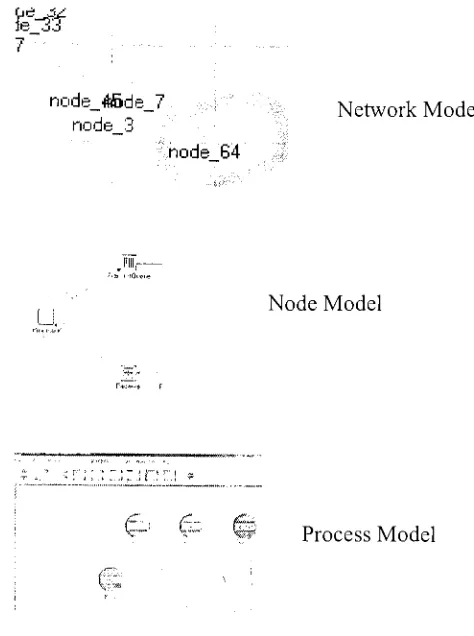
OPNET network simulation environment consists of hierarchal structure that

includesnetwork_mode, nodemodelandprocess model as shownis

fig

4.1

fe

^3

node *6de_7 _{Network Model}

node_3

node G4 ~M

J*

hbvwilbw

Node Model

Process Model

Fig

3.1

Primary Hierarchy

ofOPNET Models

The Projectmodel is themain _staging area for _creating a network simulation. From this

editor, you can build a network model _using models from the standard

library,

choose

statistics about the network, run a simulation, and view the results [5]. The Nodemodel

editor lets you define the behavior of each network object. Behavior is defined _using

different modules, each ofwhich models some internal aspect of node behavior such as

datacreation, datastorage, etc. Modules are connectedthroughpacketstreams or statistic

wires. Anetwork objectis

typically

made_upofmultiplemodulesthat_{define its behavior.}

The Process Model Editor lets us create process models, which control the _underlying

functionality

of the node models created in the Node Editor. Process models are [image:39.538.196.433.62.380.2]

represented

by

finite state machines

(FSMs),

and are created with icons that represent

states and lines that represent transitions between states. Operations performed in each

state or for a transition are

described

in embedded C or C++ code blocks [5]. There are

other editors such as Link _editor, path_editor, packet formateditor andthedemand editor

etc. These are various editors in OPNET to create link _objects, define demand models,

construct differentpackets etc.

The node _positions, timeslots and selection ofQDS nodes is done in MATLAB.

These are provided as inputs to the simulation kernel. The set of user queries, node

programs, event constraints and the simulation models

(network,

_node, and process

models) arc the other inputs provided to the simulation kernel. These inputs are then

combined with the model resources and execute the simulation.

Finally,

results are

extracted_using theExternal Model Access

(EMA)

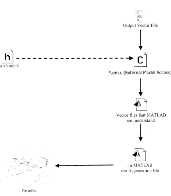
featureofOPNET and analyzed _using

MATLAB. The

following

figure

(fig 4.2)

showsthepathtoresultgeneration. Thegeneral

process used to adapt the thesis models to the available software environment was as

follows:

a. import OPNETmodels/processes

b. import OPNET scenarios

c.

debug

& fixmodel compilation errors

d.

debug

& fix crashesinmodel process simulation

e. rewritepaths and scriptsthatmanage simulation

f

debug

&fix compilationerrors of optimizedkernelexecution

g. simulateprojectwith optimizedkernel

h.

debug

& fix scriptsthatmanageEMA exportation of results

i.

debug

& fixcustomEMAprogram

j. export simulationresultsto textfilesviaEMAprogram

k.

debug

& fix MATLAB analysisprograms

analyze results withMATLAB

SensorNodc.h

Output VectorFile

I

*.em.c (External ModelAccess)

I

VectorfilesthatMATLAB

can understand

1

,mMATLAB

result generationfile

Results

Fig

4.2 processsteps ofdata extraction and resultgeneration [image:41.538.98.451.203.608.2]

4.2

Node

and

Process

Models

The node model ofthe sensor node is shown in

fig

4.3. The node consists of a

processor, a

transmitter,

areceiverand atransmitqueue. Theprocessorcontainsthe finite

state machine that controls each and _every operation of the node. The transmitter and

receiver are used for transmission ofsignals. The can transmit/receive at a rate of 2.4

Kbpsovera 80 ft

distance

andoperateinthe 900 MHZ frequency.

Also,

thenodeshavea

seismic sensorand anacoustic sensor thatare used as _sensingelements.

1

7*

Jfix

p

..TYansmitQueueTransmitter TransrnitAntenna

node 83 rY

Inn .__i_v-i

Processor Listenforspecificdatapacket whilein sleepmode

Regulardatatransfer

P

\ Receiver ReceiveAntenna

Fig

4.3 The Nodemodel of a sensor node

The transmit queue is anotherimportant part ofthenode. It isused to control the

flowofthe traffic. Whenthereis alargetrafficbetweenthetransmitterandtheprocessor,

the transmit queuehandles it inanappropriate manner. Thenodeis based onthe work of

srivastava

[9]

andthe _energyspecificationsused inthenodealsoarebasedonit. [image:42.538.91.444.274.474.2]

The process model contains the logic ofthe finite state machinethat controls the

functioning

of the node. The objects embedded are programmed in C and C++

programming

languages. OPNET provides extensive libraries to model communications

and_processingoperations.

4.3

Test

case

Scenario

A test case scenario has to be developedto test theproposals. The firsttest

case wouldbethe election ofthe

Query

Dominant Set. The firsttest caseis _arrangingthe

nodes in a disciplined manner. The arrangement was done in a hexagonal way. The

second test case involves nodes in a random way. The scenario also includes a set of

tasks which determine the_workability ofthe sensor nodes as well as the whole network.

The energy levels and performance ofthe nodes andthe total networklifetime

including

the QDS nodes are evaluated. The first test case scenario would be that of a regular

constant node density. Then we arrange the nodes in a random formation and look for

results. Before we go to see the results, we need to determine what metrics are _going to

betested.

The first metric is the _energy level of all nodes of the network. This is

obtained

by

the _calculating the total _energy ofthe network at a given time. The second

metric would bethe time spent

by

_any node in _electing a QDS node. This is the average

time of a node in thenetwork before it selects its QDS node. The other metrics include

time foraverage _energy tofall below 50% ofthe _{initial energy}andthenumber ofelected

QDSnodes. Thetestresults arebuiltandanalyzedinthe next step.

4.4

Results Analysis

The first process is to elect a

Query

Dominant Set. This set is elected in a

systematic approach as described in part 3. We take the case of 100 nodes placed in a

regular hexagonal configuration. The results were analyzed in MATLAB and we found

that the

Query

Dominantset was determined inan expectedmanner. The selection ofthe

QDS is shown in

fig

4.4. The node selection depends on the number of nodes in the

neighborhood ratherthan the distance between nodes. In the first simulation set

(fig

4.5)

we showthesimulation

id,

number of nodesandthedistance.

3C

3G /

\

-~r

3C

\_

3. 5C

>-4C /"

3C

2C

7

1C

r i ...1 1 1 i

1G 2J 5C

X Axis

hi 50 ' 30

Fig

4.4 SelectionofQDS inaregular sensor network. [image:44.538.125.409.314.607.2]

ID Number of nodes Area

1 100 100mx 100m

2 256 150mx 150m

3 400 200mx200m

4 900 300mx300m

Fig

4.5

-Parameters forsimulation

The parameters set in

fig

4.5 are taken and graph for the maximum time spent

by

_any

node _{in selecting} a QDS is displayed as is shown in

fig

4.6. The time taken is almost

constant all the time even whenthenumber of nodes increasedwiththe area. This proves

that asthe numberof nodes increasewith_{the area, the time} spent on_electinga QDS node

isconstant.

Fig. 4.6 Maximum Timespent on_{electing QDS (for}parameters

fig

4.5)

[image:45.538.106.426.49.210.2] [image:45.538.81.423.407.614.2]

Another

set ofparameters istakenwiththesamesimulation caseandistested. Inthis

parameters set we changethenumber of nodesbut

keep

theareathesame. Thisis

described

in

fig

4.7

ID Numberof nodes Area

1 100 100mx 100m

2 256 100mx 100m

3 400 100mx 100m

4 900 100mx 100m

Fig

4.7 another set of parameters

Thearea remainedthesamebutthenumber of nodes increasedin each simulation. The

result is shown in

fig

4.8

toe

Fig

4.8 Maximum Time spent on_{electing QDS (for}parameters

fig 4.7)

[image:46.538.127.423.149.305.2] [image:46.538.90.449.387.620.2]

The

aboveresult provesthat thenode

density

effectsthemaximumtime spent on _electing

the _{query dominant} set. Ifwe compare

fig

4.6 and

fig

4.8,

the maximum time is a lot

higher

becausethenode

density

has

increased

by

ahighamountinthe same given area.

The totalnetwork power isanother considerationthatneedsto beassessed. Asthe

network grows and performs _{the tasks the total power}

ultimately goes down with time.

Thepower metric

depends

onthe number oftasks assigned at_any given time. The other

factors affecting the total power is the node density. Ifthe node

density

is high and the

nodes arc placed in a systematic way, the power consumed

by

the nodes shouldbe less

than forrandom placement of nodes ifgiven the same set oftasks. The

fig

4.9 shows the

total_energyspent_along a couple ofhourswhile_performing randomtasks.

1.50

1 _5

1.00

0.50

0.25

0.00

global_battery

iTl

"O

Fig

4.9 Global Powerofthenetwork(mixedresults) [image:47.538.82.440.333.645.2]

Another

interesting

factor in theanalysisis _readinga single node in a networki.e.

arandomnodeselectedfrom thesensor network. The

following

analysisis todetermine

howmuch _energycanbe savedorlost

by

increasing

and

decreasing

thenumberoftasks

assigned and

by

making it sleep fora period oftime. The

following

aretheresults inthis

simulation.

3,000

2,000

1,000

0

2

asleeptime

batteryvalue

ia;i count

11

I

Fig

4. 10 Taskcount,

Asleep

timeand PoweranalysisI

The tasks are assigned in a haphazard way and the _sleep time was set to be

increasing

over time. The power level shown

(fig 4.10)

is _{constantly decreasing. The} results prove [image:48.538.118.426.236.562.2]

that the nodes lose power _randomly when tasks are _continuously assigned to them. The

other resultwas as thenodeisputto _sleepmode moreregularly, thepower levelremains

constant evenwhen thereis aburstoftasks assigned. The_energyremainsthesame ifthe

tasks increasewith_{increase in sleep}time

(fig.4.12)

3 000

2,000

1,000

n

2

ro lij

asleep time

batteryvalue

taskcount

0

vvmv]/)/vv

as

CO

"O

Fig

4. 1 1 Taskcount,

Asleep

timeandPoweranalysis II [image:49.538.123.426.184.512.2]

4,000

asleeptime

batteryvalue

Fig

4.12 Task count,

Asleep

timeandPoweranalysisIII

Theseare some ofthesimulation scenariosthat are addedafter

doing

athoroughresearch

onthe_way sensor nodesbehave whentasked

by

the

Query

Dominantset nodes.Thus the

results are conceived andcompared with usualprocedures and are verifiedtocheckif

they

conformto the standard norms. [image:50.538.97.391.57.379.2]

5.

Conclusion

A sensor network model _{has been developed and} analyzed in a _way that makes

sense to our aim and goals. The firstpart is an introduction towireless sensor networks,

its characteristics and issues. The primary goal of _selecting a

Query

Dominant set has

been achieved. After that the performance of the sensor network has been analyzed.

Different aspects of sensor networks

including

various _constraints, challenges and

features are discussed with emphasis to _energy conservation and simple _routing

algorithms. Although we did not

develop

a complete sensor model, some assumptions

were made to deal with all layers of networking. That is a _primary drawback for this

thesis.

The second part gives an overview of _ongoing research and development of

wireless sensors and wireless sensor networks indifferentpremium institutions.Different

network architectures that were proposed and implemented in the last few years are

discussed.

Many

solutions were developed around the world in various schools and

companies. We researched some of them and took some assumptions based on these

models.

The third part is the important piece in our work. It explains a mathematical

approach to determine a maximal independent set from Luby's Monte Carlo method. A

QDS

(Query

Dominant

Set)

node is determined withthis process which acts as acluster

head. An approach to communicate with the sensor network is also explained but not

used or tested. We assumed that the network uses the single path method in

communicating with the sink and to its _neighboring nodes. We discussed some

nodes, load balance and reliable signal transfer. The concept of single-path and

multi-path _routing techniques are _{discussed. Although} we do not use or prove _anything, we

assumesingle pathscenario inthe thesis.

The fourth part

introduces

metrics and simulation results. Here we tested the

algorithms and used a multi tool set to get to the above results. An introduction to

OPNET and the simulation parameters arc discussed. There are some metrics that are

used to evaluate our ideas such as the average _energy values of all the nodes in the

network, minimum _energy of all the nodes in the _network, total _energy consumed etc.

Some ofthe conclusionswere basedon the quantitative approach that was used to getto

them. Although the results were not the same each time the simulation were run, the

optimal solutions and results weredisplayedandtakenintoconsideration.

It is possible to do future work based on this thesis. One area where

improvements can be made is _putting the election algorithm in the node process and

testing

froma real scenario. Another study on single pathandmulti path canbe done and

implemented into this model. That will give the proposed model completeness in a

network sense. The sensornode characteristicsand features

including

itsparameters were

taken from WINS node developed

by

UCLA. Another drawback to this model is data

querying. The tasks assigned were from assumptions and not a real mode task. That can

be another improvement made to this system. A real case scenario like an animal

movement in a forest or a battlefield scenario can be taken into consideration and

implemented

by

_using this model. That would be a great project that can lead to a real

sensor model.

Also,

this model didnot take into consideration _any kind of

irregularities

like signal to noise _ratio, interference and fading. When these issues are considered the

results will _{certainly vary} and lead to some other conclusions. The sensor coverage

including

the acoustic and _sensing capabilities all are assumed and there can be

improvements

made to them. Also the

battery

can be made to have solar power

generating capability that will increase the node and networklifetime. Data aggregation

is another important factor inasensor model.

Ultimately

the end-useris concerned about

it more than _any protocols or hardware. The node placement is another factor that can

change the results. Although we worked on random and regular placements of nodes,

ideal cases were considered. There can be several other ways of

distributing

the nodes.

Also,

dead nodesordefectivenodes canbe anotherissue.

Many

improvementsneedtobe

done to provide an efficient solution to sensor network management.

Bibliography

[1]

W

Daugherty,

"The growthofwireless

mobile,"

Business

2.0,

December

12,

2000.

[2]

Di TianandNicolasD.

Georganas,

Low-

Cost,

_ReliableData

Delivery

in

Large Wireless Sensor

Networks,

SchoolofInformation

Technology

and

Engineering,

University

of

Ottawa,

2001

[3]

M. T. JonesandP E.

Plassmann,

"Aparallel graph_coloring

heuristic,"

SIAM Journal

on Scientific

Computing,

vol.

14,

no.

3,

pp.

654-669,

1993.

[4]

K.

Bult,

A.

Burstein,

D.

Chang,

M.

Dong,

andW.

Kaiser,

"Wireless integratedmicro sensors,"

Proceedings _ofConferenceonSensorsandSystems (SensorsExpo).

Anaheim,

CA, USA,

pp.

33-38,

April 16-18 1996

[5]

G.

Pottie,

"Wireless sensor

networks,"

1998Information

Theory

Workshop,

Killarney,

Ireland,

pp.

139^40,

22-26 June 1998.

[6]

R. M.

Karp

andA.

Wigderson,

"Afastparallel algorithmforthemaximal independentset

problem,"

Journal ofthe

ACM,

vol.

32,

no.

4,

pp.

762-773,

1985

[7]

O. G.

G'omez,

Efficient Parallel AlgorithmsforCombinatorial Problems. PhD _thesis,

DepartmentofComputer

Science,

Lund

University,

Sweden,

January

1996.