rsos.royalsocietypublishing.org
Research
Cite this article:
Zupo V, Alexander TJ, Edgar
GJ. 2017 Relating trophic resources to
community structure: a predictive index of
food availability.
R. Soc. open sci.
4
: 160515.
http://dx.doi.org/10.1098/rsos.160515
Received: 14 July 2016
Accepted: 10 January 2017
Subject Category:
Earth science
Subject Areas:
ecology/environmental science
Keywords:
food webs, trophic groups, feeding guilds,
abundance, resources
Author for correspondence:
Valerio Zupo
e-mail:
[email protected]
Electronic supplementary material is available
online
at
https://dx.doi.org/10.6084/m9.
figshare.c.3677065
.
Relating trophic resources
to community structure: a
predictive index of food
availability
Valerio Zupo
1
, Timothy J. Alexander
2,3
and Graham
J. Edgar
4
1
Stazione Zoologica Anton Dohrn, Integrative Marine Ecology Department, Benthic
Ecology Center, Punta San Pietro, Ischia 80077, Italy
2
Department of Fish Ecology and Evolution, Centre of Ecology, Evolution and
Biogeochemistry, EAWAG Swiss Federal Institute of Aquatic Science and Technology,
Seestrasse 79, Kastanienbaum 6047, Switzerland
3
Division of Aquatic Ecology and Evolution, Institute of Ecology and Evolution,
University of Bern, Baltzerstrasse 6, Bern 3012, Switzerland
4
Institute for Marine and Antarctic Studies, University of Tasmania, GPO Box 252-49,
Hobart, Tasmania 7001, Australia
VZ, 0000-0001-9766-8784; TJA, 0000-0002-6971-6205
The abundance and the distribution of trophic resources
available for consumers influence the productivity and the
diversity of natural communities. Nevertheless, assessment of
the actual abundance of food items available for individual
trophic groups has been constrained by differences in methods
and metrics used by various authors. Here we develop an index
of food abundance, the framework of which can be adapted for
different ecosystems. The relative available food index (RAFI)
is computed by considering standard resource conditions of a
habitat and the influence of various generalized anthropogenic
and natural factors. RAFI was developed using published
literature on food abundance and validated by comparison of
predictions versus observed trophic resources across various
marine sites. RAFI tables here proposed can be applied to a
range of marine ecosystems for predictions of the potential
abundance of food available for each trophic group, hence
permitting exploration of ecological theories by focusing on the
deviation from the observed to the expected.
1. Introduction
1.1. The importance of trophic resources
Nutrient supply and productivity gradients can strongly influence
the diversity of natural communities through trophic linkages
2
rsos
.ro
yalsociet
ypublishing
.or
g
R.
Soc
.open
sc
i.
4
:160515
...
[
1
,
2
]. Consequently, attempts to predict biodiversity patterns in marine ecosystems should consider
the abundance of food available for different trophic groups [
3
,
4
]. To date, research has been focused
primarily on influences of predators on prey populations, through a top-down approach [
5
]. Various
studies also suggest that resources and consumers interact to structure food webs [
6
,
7
] with, for example,
demonstration that herbivore and predator abundances vary predictably along natural productivity
gradients [
1
].
Unfortunately, the various forms of trophic data reported among studies impede broad-scale
comparisons because of different sampling methods, different trophic groups, incomplete sets of plant
and animal taxa, and different units of measurements [
8
,
9
]. In the marine context, benthic and planktonic
morphofunctional groups are often sampled with different instruments, on different surface areas
or volumes, and among different habitats. For this reason, only a few broad-scale cross-ecosystem
comparisons have yet been made on relationships between productivity/functioning and food resources
available for each trophic group [
3
,
5
].
1.2. Prediction of trophic resources
Nevertheless, a classification of ecosystems based on the abundance of each trophic resource is
theoretically possible [
10
]. For example, the amount of plant biomass potentially available for
macroherbivores will inevitably be much higher in seagrass meadows than unvegetated sandy substrata
or marine caves [
11
]. In addition, the abundance of food available for macrocarnivores is higher on coral
reefs than shallow seaweed meadows [
12
,
13
]. Extending such generalizations, food resources available
to different trophic groups can be evaluated by considering habitat constraints.
Various pressures acting locally also influence and modulate these general trends. For example,
the abundance of plant detritus is high in seagrass meadows, but the presence of strong currents
may disperse the detritus particles and make that resource less abundant [
14
]. Wave exposure and
associated surge also negatively influence detritus, potentially reducing availability for herbivore–
detritivores. Additionally, food for microherbivores is abundant in shallow rocky bottoms and increases
with increasing nutrients [
15
], but declines in deep rocky environments, owing to the limiting influence
of light [
16
]. Therefore, nutrient availability and depth are important moderating factors, with consistent
effects across a range of ecosystems [
17
].
Our study aims at describing general patterns of relative abundance of food available for trophic
groups among various marine habitats. Based on these patterns, we developed a mechanistic model
of food availability and validated its predictions through comparisons of computed versus observed
food resources at several comprehensively sampled sites. Trophic resources were assessed solely on the
basis of their physical presence in each habitat, irrespective of whether the food material was protected
by physical, chemical or behavioural defences [
18
]. The model is presented here in order to easily
incorporate an estimate of trophic resources in evaluations of diversity–productivity relationships [
19
]
and in other analyses of marine ecosystems.
2. Material and methods
2.1. Computation of relative available food index tables
The relative available food index (RAFI) was computed by screening the global literature on trophic
resources in marine habitats (electronic supplementary material, table S1). A literature search was
conducted using ISI Web of Science™ (
www.webofknowledge.com
) from 1945 to 2010, plus hardcopy
literature contained in the library of Stazione Zoologica, Naples, that encompasses magazine collections
from 1872 to the present. Studies involving abundance and taxonomic composition of marine organisms
were considered when the information contained was comparable and appropriate, in terms of surface
units, abundance units, substrata and taxonomic groups investigated. Restrictions related to language,
publication date or publication status were not imposed. The data recorded show regional patchiness,
owing to the availability of specific studies according to the distribution patterns of authors (
table 1
).
The first step was the evaluation of the food resources available at each of five substrata (hard, soft, hard
biogenic, macroalgae and seagrass beds;
table 2
) and for 11 trophic groups (
table 3
) that were expressed
according to the type and size of prey items [
20
].
3
rsos
.ro
yalsociet
ypublishing
.or
g
R.
Soc
.open
sc
i.
4
[image:3.522.55.468.330.425.2]:160515
...
Table 1.
Geographical distribution of the studies used for the construction of the RAFI model. The number of publications considered
for each region is reported in columns, according to various ecosystems (resulting from the classification in electronic supplementary
material, table S1), in rows. The total per cent contribution of researches performed in each region is reported in the last row.
geographical areas
biotopes
Mediterranean
Atlantic
Australian
Pacific
Pacific
Ocean
Indian
Ocean
Caribbean
Sea
China
Sea
Baltic
marine caves
1
2
1
. . . .
biogenic
3
2
3
1
. . . .
hard bottoms
4
2
1
1
1
1
1
. . . .
macroalgae
2
2
2
2
2
. . . .
seagrasses
15
7
3
1
3
2
1
1
. . . .
soft bottoms
1
3
1
1
1
. . . .
harbours
14
3
1
1
1
1
. . . .
biotope typologies
4
2
2
1
2
2
. . . .
per cent contribution
38.0
22.2
10.2
8.3
7.4
7.4
3.7
2.8
. . . .
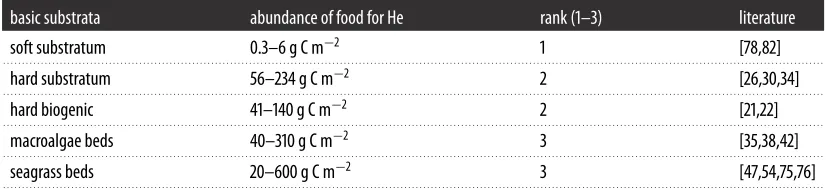
Table 2.
Example of the ranking process applied to herbivore (He) food resources for five substrata (in rows). A score from 1 to 3 is
attributed (third column) according to the ranges of abundance reported (second column). The literature used to obtain abundance ranges
is indicated in the fourth column (numbers in brackets are referred to electronic supplementary material, table S1).
basic substrata
abundance of food for He
rank (1–3)
literature
soft substratum
0.3–6 g C m
−
2
1
[78,82]
. . . .
hard substratum
56–234 g C m
−
2
2
[26,30,34]
. . . .
hard biogenic
41–140 g C m
−
2
2
[21,22]
. . . .
macroalgae beds
40–310 g C m
−
2
3
[35,38,42]
. . . .
seagrass beds
20–600 g C m
−
2
3
[47,54,75,76]
. . . .
by different authors (in various sites, seasons, etc.) were recorded. Similarly, to evaluate the abundance
of food available for macroherbivores (He) in various substrata, papers containing information on the
standing crops of plants and algae were selected for each of five habitats, and abundance data were
recorded (
table 2
, second column). Available data may be expressed in several different units (e.g.
number of individuals, mg of biomass, µg of carbon or kcal per unit surface area) according to the
methods followed by each author. In these cases, all data were converted, according to [
21
], to g C m
−
2
,
in order to permit comparisons among the different studies. Finally, the range of abundances recorded
(
figure 1
) was divided into three intervals ranked 1 (low abundance), 2 (medium) and 3 (high), as
indicated in
table 2
(third column). The interval subdivision was made according to a best professional
judgement in order to highlight the differences found among ranges.
Subsequently, each basic substratum (
table 3
a
) was further divided into specific habitats (
table 3
b
),
based on the distinctions made in most trophic models [
22
] and each food category was assigned to
an abundance interval (1–3), for each of 10 specific habitats (
table 3
b
and
figure 2
), as described above.
For example, hard substrata were grossly divided into rocky reefs and caves, according to the different
exposures to light and external influences characterizing these environments. Similarly, soft substrata
were divided into open sand and embayments, based on variable shelter influencing plant and animal
communities (
table 3
b
).
Each ecosystem was consequently classified according to the amount of food potentially available to
each trophic group (tg), according to the following relationship:
4
rsos
.ro
yalsociet
ypublishing
.or
g
R.
Soc
.open
sc
i.
4
[image:4.522.58.469.354.631.2]:160515
...
700
600
500
400
300
200
g C
m
–1
100
0
–100
soft
hard
biogenic
macroalgae
seagrass
Figure 1.
Abundances of trophic resources, expressed as g C m
−
1
, available for herbivore consumers in five different substrata. The whole
range (0–600 g C m
−
1
) has been divided into three categories of abundance.
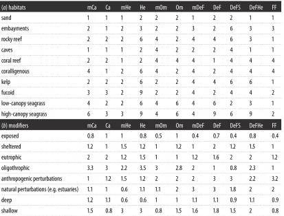
Table 3.
Computation of RAFI. The abundances of each trophic group (in columns), referring to substrata and habitats (in rows), are
derived from the available literature (electronic supplementary material, table S1). (
a
) Trophic resource abundances in relation to basic
substrata. (
b
) Trophic resource abundances in relation to specific habitats. The considered trophic groups are: microcarnivores (mCa),
carnivores (Ca), microherbivores (mHe), herbivores (He), microomnivores (mOm), omnivores (Om), microdetritus feeders (mDeF), detritus
feeders (DeF), detritus feeders–suspensivores (DeFS), Detritus feeders–herbivores (DeFHe) and filter feeders (FF).
(
a
) basic substrata
mCa
Ca
mHe
He
mOm
Om
mDeF
DeF
DeFS
DeFHe
FF
soft substratum
1
1
1
1
2
2
1
1
2
1
1
. . . .
hard substratum
1
1
1
2
2
2
2
2
2
1
1
. . . .
hard biogenic
2
1
1
2
2
2
2
1
2
2
2
. . . .
macroalgae beds
1
1
1
3
1
2
2
2
2
2
1
. . . .
seagrass beds
2
1
1
3
2
2
2
3
2
3
1
(
b
) basic substrata
specific
habitats
mCa
Ca
mHe
He
mOm
Om
mDeF
DeF
DeFS
DeFHe
FF
soft
sand
1
1
1
2
1
1
1
2
1
1
1
. . . .
embayments
2
1
2
3
1
1
3
2
3
3
3
. . . .
hard
rocky reef
2
2
2
3
2
1
2
2
3
3
1
. . . .
caves
1
1
1
1
2
1
1
1
2
1
1
. . . .
hard biogenic
coral reefs
1
2
1
1
2
2
2
1
2
2
2
. . . .
coralligenous
2
1
2
3
2
1
2
2
2
2
2
. . . .
macroalgae
kelp
2
2
2
2
2
1
2
2
3
3
1
. . . .
fucoid
3
3
2
3
2
1
2
1
2
2
2
. . . .
seagrass
low-canopy seagrass
2
2
2
2
2
3
2
2
1
1
1
. . . .
high-canopy seagrass
3
3
3
3
2
3
2
3
3
3
2
. . . .
5
rsos
.ro
yalsociet
ypublishing
.or
g
R.
Soc
.open
sc
i.
4
[image:5.522.148.372.42.207.2] [image:5.522.58.471.328.642.2]:160515
...
trophic resources
evaluated
according to 3
abundance
categories
eleven trophic
groups
1
2
3
ten habitats, eight modifiers
ecosystem
Figure 2.
Each ecosystem is classified according to 10 broad habitats and defined according to eight specific modifiers. The trophic
resources available for 11 trophic groups of consumers are evaluated according to three levels of abundance (1, low; 2, medium; 3, high).
Table 4.
(
a
) Final scores with RAFI predictions for average abundances of trophic resources in each habitat. (
b
) Modifiers for local
conditions. Trophic groups: mCa (microcarnivores); Ca (carnivores), mHe (microherbivores), He (herbivores), mOm (microomnivores),
Om (omnivores), mDeF (microdetritus feeders), DeF (detritus feeders), DeFS (detritus feeders–suspensivores), DeFHe (detritus feeders–
herbivores) and FF (filter feeders).
(
a
) habitats
mCa
Ca
mHe
He
mOm
Om
mDeF
DeF
DeFS
DeFHe
FF
sand
1
1
1
2
2
2
1
2
2
1
1
. . . .
embayments
2
1
2
3
2
2
3
2
6
3
3
. . . .
rocky reef
2
2
2
6
4
2
4
4
6
3
1
. . . .
caves
1
1
1
2
4
2
2
2
4
1
1
. . . .
coral reef
2
2
1
2
4
4
4
1
4
4
4
. . . .
coralligenous
4
1
2
6
4
2
4
2
4
4
4
. . . .
kelp
2
2
2
6
2
2
4
4
6
6
1
. . . .
fucoid
3
3
2
9
2
2
4
2
4
4
2
. . . .
low-canopy seagrass
4
2
2
6
4
6
4
6
2
3
1
. . . .
high-canopy seagrass
6
3
3
9
4
6
4
9
6
9
2
(
b
) modifiers
mCa
Ca
mHe
He
mOm
Om
mDeF
DeF
DeFS
DeFHe
FF
exposed
0.8
1
1
0.8
0.5
1
0.4
0.7
0.4
0.8
0.4
. . . .
sheltered
1.2
1
1.5
1.2
1
1.2
1
2
1.2
1.5
1
. . . .
eutrophic
2
2
1.2
1.5
1
1
1.2
1.6
2
2
1.2
. . . .
oligothrophic
3.3
3
2.2
3.5
3
2.8
2
1
0.8
2.3
1
. . . .
anthropogenic perturbations
1
1.2
1.5
1.2
2
2
2
3
3
2.2
3.2
. . . .
natural perturbations (e.g. estuaries)
1.1
1
0.6
1.1
1.1
2
3
3
1.8
2
2
. . . .
deep
1.2
1.1
0.6
0.6
1
1
1.1
1.1
0.9
1.1
0.9
. . . .
shallow
1.5
0.8
3
3
0.8
1.5
1.6
1.8
1.5
2
0.8
. . . .
6
rsos
.ro
yalsociet
ypublishing
.or
g
R.
Soc
.open
sc
i.
4
:160515
...
according to these site-specific influences (
table 4
b
) and the relationship (2.1) is set as:
Resource abundance
(tg,ecosystem)
=
f
(basic substratum
×
specific habitat)
×
specific modifiers
(2.2)
For this purpose, literature data were screened to detect deviations from ‘average’ expected conditions
under the influence of each modifier. A value of 1 was set for each trophic category under standard
conditions (
table 4
b
), meaning that the estimate of food resources, obtained in
table 4
a
, will not change.
In contrast, exposure to modifying conditions will increase or decrease the relative amount of food
resources available. For example, higher currents induce a mean decrease of 20% for the food resources
available for mCa, as determined by screening the results of studies comparing similar ecosystems
exposed to different strength currents [
28
]. Therefore, a modifying value of 0.8 was assigned in this case
(
table 4
b
).
Some modifiers produce dramatic variation from average conditions. Food resources available for
mCa may be surprisingly high (330%) in oligotrophic systems [
29
,
30
], while other trophic resources (e.g.
DeF and FF) are not influenced. This is reflected in the modifying value of 3.3 in
table 4
b
, corresponding
to the trophic resources mCa in oligotrophic environments.
These modifiers are applied only where documented local conditions strongly influence the relative
availability of trophic resources in the considered habitats. We considered ‘shallow’ habitats those in
water less than 5 m deep, and ‘deep’ habitats those located below a depth of 25 m. We considered
‘exposed’ those ecosystems open to large sea swells or characterized by very high winds, and
‘anthropogenically impacted’ those systems for which there are clear and documented evidence for major
industrial, fishery or urban pressures. Thus, only a few characterizing pressures—the most evident and
well documented—are considered for each site (see grey cells of
table 5
a
), to avoid interference with the
basic environmental features of ecosystems.
2.2. Application of relative available food index tables
To test the effectiveness of simulations provided by RAFIs, 19 different sites were chosen throughout
the world, among those for which sufficient information was provided on the abundance of food
items (permitting at least partial comparisons between computed and actual data). In fact, most studies
provide incomplete sets of trophic groups and, in this case, comparisons with the whole trophic model
provided by RAFI is not feasible. In particular (
table 5
a
), each site (in rows) was classified according to its
characteristics (in columns). The site descriptors (in each line) were set to ‘X’ when that specific feature
was applicable, and left blank (null) when the feature was not applicable (
table 5
a
). For example, ‘San
Pietro’ (the site reported in the first row) is a eutrophic (fourth grey column), shallow (last grey column)
environment in the bay of Naples (Italy), hosting a low-canopy seagrass (
Cymodocea nodosa
). In contrast,
‘N.E. St. Croix’ (the site reported in the 14th line) is a shallow, exposed coral community in the US Virgin
Islands. Each site was similarly characterized.
This classification permitted the computation of the abundance of food items (
table 5
b
), according to
the above-described RAFIs. For example, in the case of ‘San Pietro’, the values for each trophic category
were computed by multiplying all the scores previously marked with ‘X’ in
table 5
a
, i.e. the scores in line
8 of
table 4
a
(low-canopy seagrasses) by the scores in lines 3 and 8 (eutrophic and shallow, respectively) of
table 4
b
, following the relationship (2). The same computation was performed for all the other considered
sites (electronic supplementary material, table S2), according to their environment type and local specific
pressures, as reported in the literature. Repeating this procedure, the scores for each trophic category
in each site were computed (
table 5
b
). These computations are available in digital format in electronic
supplementary material, table S2, along with an empty spreadsheet to be used for the simulation of
further datasets.
Finally, the values in each cell were converted, line by line, to a percentage of the total resources
present in each site (RAFI%), in order to standardize the results and make them comparable among
different ecosystems [
31
]. Thus, RAFI% (
table 5
c
) allows comparisons among such different ecosystems
as coral reefs, temperate harbours, seagrass meadows and sand bottoms, which are characterized by
wide ranges of densities of organisms, dynamics and productivities.
10
rsos
.ro
yalsociet
ypublishing
.or
g
R.
Soc
.open
sc
i.
4
[image:10.522.55.469.83.238.2]:160515
...
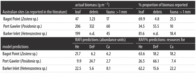
Table 6.
Comparison of trophic resources reported by Edgar & Shaw [
32
] for three Australian sites (top part) with the results of RAFI
predictions (bottom part). The proportion of trophic resources among the three main trophic groups for which experimental data were
available has been calculated. Their percentages (% proportion of biomass versus RAFI%) are compared (right part of the table).
actual biomass (g m
−
2
)
% proportion of biomass reported
Australian sites (as reported in the literature)
leaf
debris
fauna
>
1 mm
leaf
debris
fauna
>
1 mm
Bagot Point (
Zostera
sp.)
47
3.23
17
69.9
4.8
25.3
. . . .
Port Gawler (
Posidonia
sp.)
206
332
60
34.5
55.5
10
. . . .
Barker Inlet (
Heterozostera
sp.)
199
n.d.
45
81.6
n.d.
18.4
RAFI predictions (abundance units)
RAFI% predictions: resources for
model predictions
He
DeF
Ca
He
DeF
Ca
Bagot Point (
Zostera
sp.)
21.7
6.2
6.2
63.6
18.2
18.2
. . . .
Port Gawler (
Posidonia
sp.)
9.9
24.7
2.7
26.5
66.1
7.4
. . . .
Barker Inlet (Heterozostera sp.)
22.5
5.6
8.1
62.2
15.6
22.2
. . . .
Finally, a simulation for a marine protected area (MPA) in Africa, for which some literature
information is available [
33
], was performed in order to test the sensitivity of the method for computing
changes occurring after the institution of the protection plan. In this case, the factor ‘anthropogenic
perturbations’ was set to ‘X’ before the institution and ‘null’ after the institution, to perform the
simulation (electronic supplementary material, table S2).
RAFI tables were formally validated by comparing observed food resources to those predicted. For
this purpose, two comprehensively sampled sites were considered: Lacco Ameno [
34
] and Banco di Santa
Croce [
35
]. These sites were selected because (i) complete datasets were available and (ii) they host quite
different environments (
table 5
a
): seagrass versus hard bottom, eutrophic versus pristine, shallow versus
deep, etc. Fauna was sampled using an airlift sampler [
35
] in two replicate 40
×
40 cm surface area plots,
and all specimens collected were counted and identified at the species level.
Lacco Ameno (40°45
N, 13°53
E) is located in the northwest sector of the Island of Ischia (Bay of
Naples, Italy). It contains a continuous and dense meadow of
P. oceanica
extending from 1 m to about 33 m
(deep limit). Samples collected at a depth of 5 m were considered. Animals were grouped according to
their possible role as prey for macrocarnivores, microcarnivores, filter feeders, etc. Data were integrated,
when necessary, with gut content analyses evaluated for each sampled species. Prey item size was taken
into account and their abundance in the environment was evaluated based on the following relationship:
Total food biomass available
=
number of items
×
average individual biomass
(2.3)
The abundance of food available for macroherbivores and microherbivores and the actual abundance
of detritus were evaluated according to [
36
]. The results obtained were transformed into % abundance of
each food item and compared with the abundance of food items (RAFI) computed according to
table 4
.
Banco di Santa Croce (40°40
N, 14°26
E) is a submerged seamount complex located in the eastern
Gulf of Naples. It is located 0.8 km off the coast and is composed of various rocky seamounts arising
from a depth of 60 to 11 m, forming a circular structure. Samples were obtained over a 3 year extensive
sampling programme to develop a trophic model for the site [
37
]. Direct measurements provided the
actual abundance of food items and the abundance of species of each trophic group per square metre.
The total number of individuals per m
2
, as well as the total biomass of each trophic group and abundance
of organic detritus and of phyto- and zooplankton were also available [
37
], and converted into the same
units to allow direct comparisons. The fish fauna was surveyed using visual census [
37
].
2.3. Statistical analyses
The
r
2
coefficient was calculated using correlation analysis to evaluate how well the RAFI predictions
for each trophic group fitted data for the selected sites derived from the literature. The results were
confirmed by the
G
-test (likelihood ratio test).
11
rsos
.ro
yalsociet
ypublishing
.or
g
R.
Soc
.open
sc
i.
4
:160515
...
30
20
10
0
ab
undance (%)
ab
undance (%)
30
Banco Santa Croce
Lacco Ameno
20
10
0
categories
RAFI%
actual
mCa
Ca
mHe
He
mOm
Om
mDeF
DeF DeFS
DeFHe
FF
mCa
Ca
mHe
He
mOm
Om
mDeF
DeF DeFS
DeFHe
FF
(
a
)
(
b
)
Figure 3.
(
a
) RAFI simulation and actual per cent abundance of resources available for various feeding groups, obtained for Lacco Ameno
(Ischia Island, Italy); (
b
) RAFI predictions and actual per cent abundance of resources available for various feeding groups, obtained for
Santa Croce Bank (Bay of Naples, Italy).
between RAFI estimated and observed food resources at the sites for which complete data across all
trophic groups were available. For all the other sites, RAFI predictions were qualitatively compared with
the available literature data, even when incomplete, by detecting the dominant food resources predicted
by RAFI and their correspondences with the dominant food resources described in the literature.
3. Results
3.1. Relative available food index validation
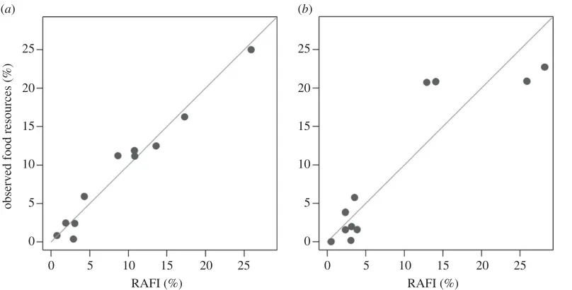
The comparison of the abundances of food items estimated by means of the proposed method with
field data shows some differences, but trends coincide (
figure 3
). In particular, data for Lacco Ameno
d’Ischia (
figure 3
a
) show good agreement between RAFI% simulated data and observed data, other
than carnivores (Ca), which appear to be overestimated by RAFI. As for the other trophic categories,
herbivores, DeF and DeFHe, as well as mDeF, are slightly higher when calculated by RAFI, whereas
mCa, mHe, Om and DeFS are slightly lower than actual. The most abundant resource is macroherbivore
food, accounting for about 25% of the total trophic resources available, followed by DeFHe (about
15%), omnivores, mHe and mCa (about 10%). On the whole, the relationship between actual and RAFI
estimated data was highly significant (
figure 4
a
,
r
2
=
0.97).
12
rsos
.ro
yalsociet
ypublishing
.or
g
R.
Soc
.open
sc
i.
4
[image:12.522.66.470.41.246.2]:160515
...
25
20
15
10
observ
ed food resources (%)
5
0
25
20
15
10
5
0
0
5
10
15
RAFI (%)
20
25
0
5
10
15
RAFI (%)
20
25
(
a
)
(
b
)
Figure 4.
Observed values of per cent abundance for trophic resources versus RAFI% estimated values for resources present in two
Mediterranean sites. The grey line denotes 1 : 1 agreement between the two methods. (
a
) Lacco Ameno;
t
=
15.72, d.f.
=
9,
p
-value
<
0.001,
r
2
=
0.97. (
b
) Banco di Santa Croce;
t
=
6.38, d.f.
=
9,
p
-value
<
0.001,
r
2
=
0.82.
(
r
2
=
0.82 between predicted and field data;
figure 4
b
), apart from some variability observed in individual
categories.
Similarly,
t
-tests indicated no significant differences (
p
<
0.001) between the RAFI data simulated for
three Australian sites hosting seagrass meadows and field data, according to the known feeding groups
investigated (
table 6
and
figure 5
). In addition, data reported in the literature on the abundance of the
main trophic groups were compared with the results of RAFI predictions for various sites (
table 7
), with
good coincidence.
Finally, the simulation of the Sine Saloum MPA [
33
] produced clear differences before and after the
institution of the protection plan. In particular (
figure 6
), the resources available for microcarnivores,
carnivores, herbivores and omnivores showed an increase in the protected conditions, whereas the
trophic resources available for detritus feeders and herbivore–detritus feeders exhibited a decrease after
the institution of the MPA (i.e. in the absence of ‘anthropogenic influences’).
3.2. Test of relative available food index in various sites of the world
The trophic resources available at various sites were predicted by RAFI and clear distinctions were
obtained, according to specific ecological conditions, even when similar ecosystems were considered.
Comparing the trophic resources available in three sites hosting seagrass meadows (San Pietro, Castello,
Port Gawler), we observed very different patterns of resource distribution (
figure 7
). In San Pietro, which
hosts a low-canopy seagrass bed (
C. nodosa
), most trophic resources are available for herbivores (26%),
followed by detritus feeders (16%), detritus feeder–herbivores and microcarnivores (11%). In contrast,
in Castello d’Ischia, an acidified site hosting a high-canopy seagrass (
P. oceanica
), most trophic resources
are available for detritus feeders (35%), followed by DeFHe (22%) and DeFS (10%). The Australian Port
Gawler site hosts a
Posidonia
sp. meadow and exhibits maximum abundance of resources for detritus
feeders (25%) followed by DeFHe (16%) and DeFS (10%), showing the importance of plant detritus in
this Australian seagrass ecosystem.
3.3. Relative available food index trends in various environments
13
rsos
.ro
yalsociet
ypublishing
.or
g
R.
Soc
.open
sc
i.
4
[image:13.522.151.373.34.543.2]:160515
...
90
80
70
60
50
40
30
20
10
0
90
80
70
60
50
ab
undance (%)
ab
undance (%)
ab
undance (%)
40
30
20
10
0
90
80
70
60
50
40
30
20
10
0
He
DeF
Ca
He
DeF
Ca
He
DeF
feeding guilds
RAFI%
E&S
Ca
(
a
)
(
b
)
(
c
)
Figure 5.
Comparison of the results reported by Edgar & Shaw [
32
] on the abundance of trophic resources for He, DeF and Ca. Edgar &
Shaw [
32
] data (E&S) are indicated by grey bars, against predictions of the RAFI model (RAFI%, white bars). Three sites are considered,
for which sufficient literature data were available: (
a
) Bagot Point, (
b
) Port Gawler and (
c
) Barker Inlet.
and sensitive to the effect of specific modifiers, in the considered environments. In fact, according to
RAFI, the abundance of food available for FF accounts for 4% of the total trophic resources in some caves
(Grotta del Mago), and in an analogous environment (Formiche) it declines to 1% of the total trophic
resources.
4. Discussion
4.1. The accuracy of model predictions
14
rsos
.ro
yalsociet
ypublishing
.or
g
R.
Soc
.open
sc
i.
4
[image:14.522.56.470.94.494.2]:160515
...
Table 7.
Comparison of predicted RAFI% and abundance of trophic resources derived from the available literature. For each site, the
most abundant trophic groups identified by RAFI% are indicated in the second column. The most abundant trophic group (TG) or trophic
resources (TR) reported for each site in the literature (fourth column) are provided in the third column. Country abbreviations are Italy,
IT; United States Virgin Islands, US; Costa Rica, CR; New Zealand, NZ.
site
RAFI-predicted
highest trophic
resource(s)
most abundant trophic
resources (TR) or trophic group
(TG) according to the literature
references (electronic
supplementary
material, table S1)
San Pietro (IT)
He
herbivorous molluscs (TG)
[131]
. . . .
San Pietro (IT)
DeF
detritivorous polychaetes (TG)
[132]
. . . .
Bell’Ommo (IT)
DeF, DeFS
gorgonians (TG)
[133]
. . . .
San Pancrazio (IT)
He, mHe
algae (TR)
[134]
. . . .
Secca La Catena (IT)
He, DeF
algae (TR)
[135]
. . . .
Pizzaco (IT)
He
algae (TR)
[135]
. . . .
Pizzaco (IT)
DeF, DeFS, DeFHe
gorgonians (TG)
[135]
. . . .
Grotta del Mago (IT)
DeF
detritus feeding amphipods (TG)
[136]
. . . .
Grotta del Mago (IT)
DeFS
sponges (TG)
[137]
. . . .
Formiche (IT)
He
algae (TR)
[138]
. . . .
Formiche (IT)
mHe
diatoms (TR)
[138]
. . . .
Formiche (IT)
Om
both animal and algae associations (TR)
[138]
. . . .
Maronti (IT)
DeF, mHe
detritus and plant material (TR)
[139]
. . . .
Maronti (IT)
He
drift algae (TR)
[140]
. . . .
Porto d’Ischia (IT)
DeF
organic detritus (TR)
[141]
. . . .
Porto d’Ischia (IT)
He
algae (TR)
[142]
. . . .
Cava dell’Isola (IT)
DeF
seagrass and detritus (TR)
[143]
. . . .
Castello (IT)
DeF
sea urchins (TG)
[144]
. . . .
Castello (IT)
He
herbivorous fishes (TG)
[145]
. . . .
Castello (IT)
DeFHe
DeFHe (TG)
[146]
. . . .
N.E. St. Croix (US)
He, DeFHe
herbivores (TR)
[147]
. . . .
Chatham Island (NZ)
mDeF, He
detritus feeders and herbivores (TG)
[148]
. . . .
Dos Amigos (CR)
Om, DeF
DeF and Om echinoderms (TG)
[149]
. . . .

![Figure 5. Comparison of the results reported by Edgar & Shaw [32] on the abundance of trophic resources for He, DeF and Ca](https://thumb-us.123doks.com/thumbv2/123dok_us/8409096.327358/13.522.151.373.34.543/figure-comparison-results-reported-edgar-abundance-trophic-resources.webp)


