Complex structures in media displaying electromagnetically induced transparency : pattern multistability and competition

pattern multistability and competition

1 _{Photonics Group, Research Institute for Applied Physics and Astronomy, University of Tabriz, Tabriz, Iran and} 2

SUPA and Department of Physics, University of Strathclyde, Glasgow G4 0NG, Scotland, UK

Spatially periodic and localized structures in the transverse plane of a medium displaying elec-tromagnetically induced transparency in an optical cavity and under the action of two pumps, are investigated. The system supports a multitude of different complex spatial structures depending on the chosen initial condition. We explore regimes of multistable patterns, filaments, stable defects, scrolling structures, nested patterns, fronts and the spontaneous occurrence of multiple cavity soli-tons. To simulate realistic conditions of operation, we replace periodic boundary conditions with pumps of finite size. Many of the multistable features are recovered apart from the scrolling of patterns with defects.

PACS numbers: 42.50.Lc, 42.50.Dv, 42.65.Yj

I. INTRODUCTION.

Formation of regular and localized structures in spa-tially extended systems far from thermodynamical equi-librium has been the subject of a vast number of re-searches in the past two decades [1–5]. For optical sys-tems spatio-temporal phenomena arise in the structure of the electromagnetic field in the plane orthogonal to the direction of propagation as a result of the nonlin-ear response of the materials to intense laser beams and the spatial coupling provided by diffraction. Diffraction in the paraxial approximation is described by a trans-verse Laplacian operator. Particularly interesting is the case of nonlinear materials contained in optical cavities under the action of external pumps. In the mean field approximation, such systems are described by complex partial differential equations [3, 5, 6] with two spatial dimensions plus time. Stationary solutions of partial dif-ferential equations can be seen as single points in an infinite dimensional phase space. The identification of families of coherent structures (or modes) allows, how-ever, to reduce the infinite degrees of freedom to a finite number of relevant variables and move within a finite-dimensional sub-space. When a bifurcation occurs, the associated unstable trajectories move away from the orig-inal stationary point but remain typically confined to a lower dimensional sub-space of the fully available volume. This sub-space is attracting in the sense that trajectories starting outside such space will converge to it, so that the degrees of freedom outside the attractors are effectively irrelevant [7, 8]. It is for this reason that it is possible to describe several pattern-formation problems near thresh-olds of instability with a limited number of families of solutions (modes). After an instability has produced a growing disturbance from one of the stationary modes, intrinsic nonlinearities move the system toward a new

∗_{Electronic address: [email protected]}

state. In some cases local disturbances grow to finite amplitudes and the new state resembles a deformation of the original structure with stable defects. In other cases, the new structure, that can be a stationary state or a dy-namical regime (including spatio-temporal chaos), looks nothing like the linearly unstable deformation from which we have started [9]. The system may evolve in entirely new directions as determined by the nonlinear dynam-ics, multistable solutions and the initial condition. The importance of initial conditions for the asymptotic be-haviour of the system is well-known from the basic con-cepts of nonlinear dynamics and complex systems. In our case sensitivity to initial conditions means that each point in phase space may be very close to other points with significantly different future evolutions. Thus, an arbitrarily small perturbation of the current trajectory may end in one of the many stable solutions. Once the evolution has stabilized, memory of the initial condition can affect the sequence of bifurcations of the asymptotic structure observed when changing a control parameter.

The complex spatial structures forming in nonlin-ear cavities displaying electromagnetically induced trans-parency (EIT) [10] show generalized multistability of the kind described above. In particular, it will be shown that different spatially periodic structures (optical patterns) are obtained for different initial conditions but the same parameter values. Local perturbations lead to stable pat-terns with defects. When changing a control parameter the sequence of observed structures including distorted, oscillating and scrolling (DOS) solutions displays mem-ory of the chosen initial condition. These effects survive the presence of optical pumps of finite size. The simul-taneous presence of a multitude of extended and local-ized spatial structures, defects, disorder, front instabili-ties and filamentation provides EIT media in optical cav-ities with unique flexibility and control of operation with possible applications in optical processing of information, novel memory functions and self-organized compensation of diffraction.

2

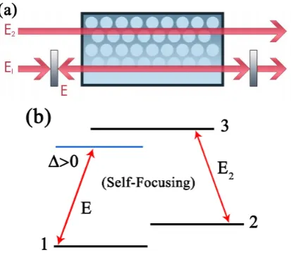
FIG. 1: (Color online) (a) The cavity configuration with the three-level atomic medium and the holdingEI and coupling

E2 beams. (b) The Λ atomic scheme with two ground states

|1>,|2>and a single excited level|3>.

model and associated equations are discussed in section 2 along with the stationary solutions and their stabil-ity analysis. Section 3 describes the variety of solutions obtained by using different initial conditions. We then describe the spontaneous appearance of a cavity soliton gas in Section 4 while the effects of finite pump are pre-sented in Section 5. Conclusions and topics for future research are discussed in Section 6.

II. THE MODEL.

The system of interest is a Fabry-Perot type cavity filled with 3-level atomic vapour (for example Rb atoms) in a Λ configuration and under the action of two opti-cal pumps. The schematic representation of the cavity and the configuration of atomic vapour are shown in Fig. 1. The injected field EI (holding beam) is detuned by ∆ from resonance of the atomic transition|3>→ |1 >

while the coupling beam E2 is kept at resonance with the transition|3>→ |2>. The cavity mirrors resonate the field E which is detuned form the injection EI by

θ. In the present model the field E2 is not resonated in the cavity which is realistic if the atomic frequencies are well separated. Many EIT experiments, however, use the ground states of alkali atoms with a small frequency dif-ference (few GHz) between the two optical fields. In such cases, polarizing beam splitters can be used to introduce orthogonal polarizations so that the coupling beamE2is not oscillated in the cavity [11].

The mean field equation for a beam propagating in the Λ medium inside the optical cavity of Fig. 1 is [10]:

∂tE=EI−(1 +iθ)E−2iCρ13+i∇2E (1)

whereE is the complex intra-cavity field,EI is the nor-malized amplitude of the pump field (considered to be a real function without loss of generality),θ is the detun-ing between the cavity resonance and the frequency of the injected pump beam, andρ13is the off-diagonal den-sity matrix element proportional to the field amplitude

Eand the complex susceptibilityχ via the relation

ρ13=χE =

∆|E2|2 |E2|2+|E|2−i∆

(|E2|2+|E|2)

3 E . (2)

Cis the co-operative parameter directly proportional to the atomic densityna through

2C=naµ 2_kL

2~γ0T

, (3)

where µ is the atomic transition dipole moment, k the wave number of the field,Lthe length of the cavity,γthe atomic linewidth,0the permittivity of free space, andT is the cavity mirror transmittivity. The diffraction term is given by the Laplacian operator in two transverse di-mensions and time is normalized to the photon life time. Details of the derivation of the diffractive Maxwell-Bloch equation (1) for the case of a two-level medium are pro-vided in [6, 12]. Equation (1) is a generalization of the model introduced in [10] since in the evaluation ofρ13we used a less stringent condition of|∆|2_<<|E

2|2 instead of|∆| << |E2|2. The bistable nature of the light-atom interaction and the capability of the system for display-ing EIT in the present model (1) are extended to a wider parameter space than that of [10] (see for example Fig. 2 where the complex susceptibility and the input-output curve are displayed in (a) and (b), respectively). Note that the detuning parameter ∆ is here considered to be positive indicating the self-focusing regime. The homo-geneous steady states are given by the implicit complex equation

EI = (1 +iθ)Es+

2iC∆|E2|2 |E2|2+|Es|2−i∆

(|E2|2+|Es|2)

3 Es

(4) whereEsis the steady value of the intra-cavity complex field. The linear stability analysis of the homogeneous steady state solutions determines the Turing instabil-ity domain where they bifurcate to patterned structures. The characteristic equation for the critical wave-vector

K of the patterned structures is obtained from linear stability analysis calculations and is given by

K2 = −

"

θ+2C∆|E2| 2 _|E

2|2− |Es|2

(|E2|2+|Es|2) 3 # (5) ±    "

2C∆|E2|2|Es|2

(|E2|2+|Es|2) 3

#2"

4 + 9∆

2

(|E2|2+|Es|2) 2

#

− "

1 +2C∆ 2_|E

2|2 |E2|2−2|Es|2

(|E2|2+|Es|2) 4

#2 



1/2

FIG. 2: (Color online) (a) The imaginary (solid line) and real (dashed line) parts of the complex susceptibility χ for

|E|2

= |E2|2

= 1. (b) Bistability in the input and output intensities for ∆ = 0.2,θ=−1,|E2|2

= 1 and 2C= 20.

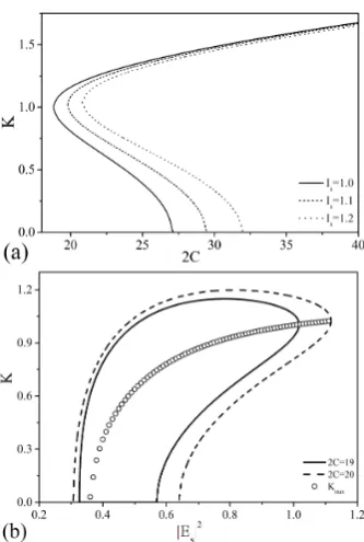
For example, for the set of parameter values chosen in Fig. 2 (b), the dashed line indicates the region where the homogeneous solution leads to patterns while in Fig. 3 (a) the Turing bifurcation point occurs at 2C = 18.8 forIs=|Es|2= 1. The range of unstable wave-vectors is displayed in Fig. 3 (b) where the entire region enclosed in the curves is Turing unstable. In Fig. 3 (b) we also display the line corresponding to the wave vector with maximum growth rate:

K_max2 = 2C∆|E2| 2_(|E

s|2− |E2|2)−θ(|Es|2+|E2|2)3 (|E2|2+|Es|2)3

.

(6) It is obvious that for the case of Is =|Es|2=|E2|2 one obtains a straight line atKmax=

√

−θ not displayed in Fig. 3 (a).

Although the fundamental mechanism of spatial cou-pling in optics is diffraction instead of diffusion, the na-ture and character of the pattern forming instabilities displayed here are the same of those introduced by Alan Turing in 1952 [13] as discussed in [14].

III. MULTISTABLE SPATIAL STRUCTURES

We have numerically integrated Eq. (1) by using a split-step method where we separate the algebraic and Laplacian terms and solve the time derivative term by a Runge-Kutta algorithm and diffraction term by Fast Fourier Transforms. Simulation grids up to 256x256

FIG. 3: Turing instability domains for pattern formation of wave-vectorKversus increasing 2C(a) and versus increasing stationary intensities (b). Parameter values are ∆ = 0.2,

θ=−1,|E2|2 _{= 1. In (a) |E}

s|2 = 1 (solid line),|Es|2 = 1.1

(dashed line) and|Es|2 = 1.2 (dotted line). In (b) 2C = 19

(solid line) and 2C= 20 (dashed line). The line traced by the small circles determines the wave-vector of largest growth for 2C= 20.

points have been used while changing the control param-eter 2C that can be modified experimentally by increas-ing or decreasincreas-ing the atomic density na. In what fol-lows three regimes based on different initial values of the control parameter are discussed, each of them display-ing separate characteristics for the observed sequence of solutions. Parameter values are kept fixed at ∆ = 0.2,

θ=−1,|E2|2= 1 and|Es|2= 1 unless stated otherwise.

A. Stable periodic patterns

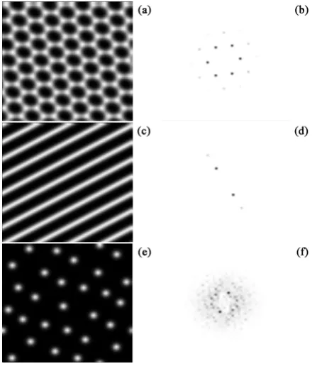
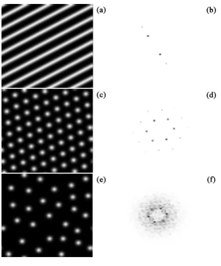
The bifurcation point of the homogeneous solution to patterns in Fig. 3 (a) is 2C= 18.8. In the first scan the initial value of 2Cis selected below the bifurcation point. This leads to the sequence of stable patterns changing from honeycombs to rolls and from rolls to spontaneous cavity solitons towards the end of the instability interval. Stable honeycombs start at 2C = 18.8 and end at 19.8, stable rolls start at 2C = 19.9 and end at 21.61, cavity solitons are observed between 2C = 21.62 and 21.6265. Examples of these patterns along with their far-field im-ages are shown in Fig. 4 for 2C= 19.6 (a)-(b), 2C= 21.0 (c)-(d) and 2C= 21.62 (e)-(f).

inten-4

FIG. 4: (a) Stable honeycomb structures for 2C = 19.6, (c) stable roll patterns for 2C = 21.0, (e) cavity solitons for 2C = 21.62 with (b), (d) and (f) their far-field images re-spectively. Note that in (b), (d) and (f) the central point has been removed to increase clarity of the images.

sities are shown in Fig. 5 versus the corresponding input intensity|EI|2.

B. Distorted and scrolling structures

We turn our attention to a starting point of the simu-lations just after the Turing instability point (2C= 18.9 for our selected parameter values). A graph showing the sequence of different transverse structures and their in-tensities versus changes of the control parameter 2C is shown in Fig. 6. Structures with different characteristics from the regular patterns described above are observed from the very beginning of the scan. The black squares in Fig. 6 correspond to honeycomb patterns with stable defects that alter their spatial periodicity. For example in Fig. 7 we present a stable honeycomb structure, dis-torted by defects, and its far field distribution obtained by starting from random initial conditions. In general, defects appear when there are more than one attracting solution in the dynamics of a given system. If the initial condition puts the spatial configuration of the field some-where between the attracting solutions, stable fronts and defects between the two patterns can form as described for example in chapter 7 of [1]. In the cases where the two attracting solutions are the same pattern but with different wave-vectors, formation of defects are expected

FIG. 5: (Color online) The instability domain of the 2C pa-rameter versus the input intensity (lower part and left axis) and the corresponding maximum intensities for different pat-terns (upper part and right axis).

FIG. 6: (Color online) The instability domain of the 2C pa-rameter versus the input intensity (lower part and left axis) and the corresponding maximum intensities for different pat-terns (upper part and right axis) when starting at 2C= 18.90. ”DOS” stands for Distorted-Oscillating and Scrolling.

while for the case of two different patterns associated to the attracting solutions, nested patterns can form [15] as discussed in the next subsection.

os-FIG. 7: (a) The distorted honeycomb pattern (left) and its far-field image (right) for 2C = 18.84. The yellow circles identify the position of defects. Note that these patterns with defects maintain their spatial shape basically unchanged when turning into scrolling structures.

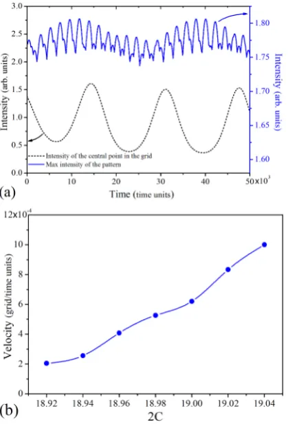
FIG. 8: (a) Oscillation of the maximum intensity of a scrolling pattern with defects (solid line) and in the central point of the structure (dotted line) for 2C = 19.0. (b) Speed of the scrolling patterns versus 2C.

cillation of the maximum intensity (solid line) that has a frequency around 8 times larger than that of the scrolling motion. When increasing 2Cfurther, the scrolling speed increases (see Fig. 8 (b)) until locking takes place again. Two ranges of scrolling structures have been found in the simulations of Fig. 6, from 2C = 18.88 to 18.89 and from 2C = 18.92 to 19.04. When increasing further the control parameter 2C, regular honeycombs are retrieved although with different orientation and slightly different

FIG. 9: Stable fronts separating roll patterns nested in a honeycomb structure (a) and their far-field image (b) for 2C= 19.6.

wave-number than those described in III A. When these become unstable, roll structures are formed but with an intensity and a wave-vector widely different from those observed in III A. This is not surprising since the number of stable wave-vectors increases with 2Cas shown in Fig. 3. When finally roll patterns lose stability, the regime of soliton gas has a stability range and intensity differ-ent from what has been observed above, thus confirming the sensitivity of the observed structures and bifurcations upon the initial conditions of the scan.

C. Bistable patterns and wavy rolls

Setting the initial value of the control parameter 2C

ho-6

FIG. 10: (Color online) The sequence of patterns in input intensity versus 2C space and the corresponding intensities for different patterns (right axis). These were obtained for an initial value of 2C=19.60.

FIG. 11: Wavy roll pattern (a) and the corresponding far-field image (b) for 2C= 19.9.

mogeneous state. This means that the roll patterns of Figs. 5, 6 and 10 have wave-vectors different from that of maximum growth. When approaching the end of the Turing unstable regions for large values of 2C, straight roll structures can encounter different instabilities that are wave-vector dependent such as Eckhaus, cross-roll, zig-zag and skewed-varicose instabilities [1, 4, 18]. De-pending on the selected wave-vector of the roll structure of a particular scan, straight rolls may remain stable un-til the end of the Turing region (see Fig. 10) or lose their stability to, for example, gases of cavity solitons (see Figs. 5, 6) as discussed in the next subsection. Al-though there are similarities with what is observed in standard models such as Swift-Hohenberg [1, 4], Brus-selator [1, 19] and Lugiato-Lefever [6], we note that in our case the stable homogeneous state for large 2C is attained through a saddle-node bifurcation atK= 0 in-stead of a Turing mechanism at finite wave-vector. We note that different instabilities for the same pattern with different wave-vector is not limited to the roll structures as discussed for example in [4] and in [20] for nonlinear optics.

The issue of different instability for the same pattern but different wave-vector is not limited to the roll struc-tures discussed here and there are detailed studies that

FIG. 12: (Color online) Deviations of the wave-vectors from that of maximum growth as a result of starting the scan at different distances from the threshold. Note that these values are for pure patterns, i.e. stable honeycombs forming before 2C=20 and rolls thereafter. The missing parts in the curves are related to distorted honeycombs, bistable patterns and wavy rolls.

show such processes can happen for states that are pe-riodic in two or more extended variables such as two-dimensional lattice states, see for example section 4.2 and 4.3 of [4] for discussions on stability balloon.

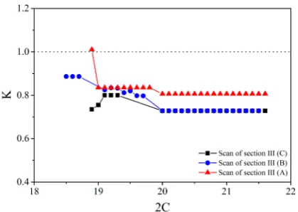
The differences among the wave-vectors obtained in the three different scans presented above can be appreci-ated in Fig. 12. These curves confirm that the presence of pattern bistability and stable defects prevent the system to relax to the structure of maximum growth rate when changing a control parameter that simulates experimen-tal realizations.

D. Spontaneous formation of a gas of cavity solitons

struc-FIG. 13: Spontaneous formation of a gas of cavity solitons. We start from a roll solution (a)-(b), and then cross an un-stable distorted hexagonal pattern (c)-(d) to finally reach the stable cavity soliton gas (e)-(f). Parameter 2C= 21.62.

ture with a saddle stability and that later leads to the formation of the soliton gas. The sequence of events is also displayed in the far-field images of Fig. 13 for clarity. During the transition from rolls to cavity soltions consid-erable variations of the maximum and minimum intensi-ties are observed. Note also that the final number of cav-ity solitons is considerably smaller than the number of peaks of the unstable distorted hexagonal structure. By further increasing the control parameter 2Cone observes a progressive reduction in the number of solitons in the gas. Unlike the formation process which is accompanied by the merging of unstable hexagonal pattern peaks, dis-appearance of CSs occurs for individual CSs in the gas. Finally, the last cavity soliton disappears and the sta-ble homogeneous state is recovered. Note that the CS merging process is intrinsically associated to dissipation of energy since in the presence of conservation, solitons travel through each other or form bound states [21].

As the cavity soliton gas loses its peaks, the peak inten-sity of the solution also reduces along with an increase in the minimum intensity value. However, the minima of the CS intensity remains well below the intensity of homogeneous state.

It is interesting to see what happens when decreas-ing the control parameter 2C starting from a soliton gas state. As shown in Fig. 14 one observes first an increase in the number of cavity solitons and then the appear-ance of filaments until the transverse space is covered by

FIG. 14: Formation of filaments from stable cavity soliton gas by decreasing the control parameter. 2C = 20.88 (a), 2C= 20.69 (b) and 2C= 20.65 (c).

almost periodic structures made of filaments. Note that filament structures are bistable with regular rolls and fur-ther increase the number of multistable states of the EIT system.

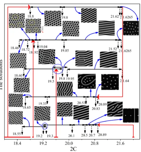
Finally, in Fig. 15 we show the great variety of possible transverse structures that can be observed when changing the control parameter 2C and the selected initial condi-tion in an absorber close to EIT in a cavity. It is evident that the effect of initial condition includes the range of stability of pattern solutions, the presence or absence of stable defects, the appearance of special structures like wavy rolls, filaments or spontaneous cavity solitons, the onset of scrolling patterns and the overlap of two dis-tinct pattern solutions. We note that this rich variety of structures and behaviour is not restricted to optics but is a universal feature of spatio-temporal nonlinear sys-tems and has been observed for example in models for the calcification of the heart tissue [22].

IV. FINITE SIZE INPUT PUMP

To understand the physical relevance in optics of the multistable solutions described in the previous section, it is important to investigate the effect of periodic boundary conditions used in the simulations. This can be properly done by comparing the previous results with those ob-tained in simulations with an input pumpPI(r) of radial shape and finite size. This makes the situation closer to possible experimental realizations. In order to maintain a large aspect ratio in the transverse plane we have used a hyperbolic tangent profile which simulates a flat-top injected beam with rapidly vanishing tails:

PI(r) =

EI

2 {1−tanh[σ(r−r0)]} (7)

whereσandr0regulates the size of the tail and flat part of the pump, respectively. PI(r) replacesEI in Eq. (1). A grid of 128x128 points and size of 20λcis used although checks on a 256x256 grid have been performed too.

8

FIG. 15: Different progression of solutions as a consequence of selecting different initial conditions. The structures are sta-ble honeycomb, stasta-ble roll, cavity solitons, distorted honey-comb, scrolling honeycombs, coexisting roll-honeycomb and wavy rolls respectively. Dashed arrows show the threshold for the patterns of the type which solid and longer arrows are pointed at. The sequence of scan in 2C for each set is shown by the arrows connecting the initial value, either from noise (points on the horizontal axis) or by using the memory of the last solution of a branch, to the set of solutions in branches. Note that cavity solitons are in a regime where the homo-geneous background is stable, as seen from the right lower most sequence of solutions which starts from noise and shows the stability of homogeneous branch up to 2C=20.89 where a saddle-node bifurcation occurs.

and localized structures displayed in Fig. 15 have found a counterpart in the simulations with circular injection. For example Fig. 16 shows patterns with defects, fronts between rolls and honeycombs (see [15] for a roll-hexagon structure with circular boundaries), filaments and cavity soliton gases respectively.

Of particular importance for our investigation is the robustness of the coexistence of rolls and honeycomb terns. Fig. 16 (b) shows an example of stable roll pat-terns coexisting with honeycomb structures in the pres-ence of a finite size injected pump. The introduction of two new parameters in the pump specification puts fur-ther emphasis on the crucial role of initial conditions in determining the final solutions and their sequence from the simple Eq. (1) because of generalised multistability of structures.

Differing from other multistable structures, the spon-taneous scrolling motion of distorted patterns disappears as soon as one employs a finite pump size. The defects

FIG. 16: Examples of transverse structures with a finite pump size withσ= 1.67/λcandr0= 9λc. Honeycomb with defects

(2C = 18.95) (a), coexistent honeycomb and roll structures (2C= 19.6) (b), filaments (2C= 20.50)(c) and gas of cavity solitons (2C= 21.55) (d).

which are intrinsic to scrolling strictures [16] are instead a robust feature that survives the external imposition of circular symmetry as demonstrated in Fig. 16 (a).

V. CONCLUSION

Complex and multistable spatial structures forming in the self-focusing regime of a cavity close to EIT are discussed. The multistability of the model is explored by putting emphasis on the importance of initial condi-tions. Particularly, three routes of solutions are studied by numerical simulations proving unique properties for each. It is seen that the selection of initial value for the control parameter can affect the range of pattern solu-tions, presence or absence of specific patterns and their behaviours. We have also investigated nested patterns formed of stable rolls and honeycomb structures sepa-rated by stable fronts. Wave vector dependant roll insta-bility is the mechanism responsible for the spontaneous formation of a gas of cavity solitons. Finally, the homoge-neous pump has been replaced with a finite size injection to remove the effect of periodic boundary condition and check the robustness of the multistable solutions. All survived, showing their physical relevance in experimen-tal conditions, with the exception of distorted scrolling patterns.

The multistability and rich variety of solutions are not a consequence of the specific selection of the parameters that have been kept at fixed values, i.e. ∆,θ,|E2|2 and

in the nature and bifurcations of the spatial structures observed. The generalized multistability observed here is a consequence of the feedback provided by the cav-ity mirrors and is expected to affect the output of the system even when medium propagation effects are taken into consideration. Propagation of light in media display-ing EIT without a cavity leads to manipulation of the susceptibility in momentum space, slow light and even elimination of diffraction [23]. Coupling these features with our transverse cavity effects may offer a flexibility of operation that is unprecedented in nonlinear optical devices.

Finally, the onset and interaction of localized solutions such as cavity solitons and filaments in the EIT model

appears to be different from what is observed in typical optical pattern formation with third order and second order nonlinearities. The transition from cavity solitons to filaments, the long range interaction of the solitons and the processes of control and use of localised solutions in photonic devices that display EIT will be the subject of future communications.

Acknowledgements

DM acknowledges EPSRC for support.

[1] D. Walgraef, Spatio-Temporal Pattern Formation, (Springer-Verlag, Berlin, 1997)

[2] L. A. Lugiato, M. Brambilla, and A. Gatti, Adv. At. Mol. Opt. Phys.40, 229 (1999)

[3] T. Ackemann and W. J. Firth, in Dissipative Solitons

edited by N. Akhmediev and A. Ankiewicz, Lecture Notes in Physics,661(Springer-Verlag, Berlin, 2006) page 55 [4] M. C. Cross and H. S. Greenside,Pattern Formation and

Dynamics in Nonequilibrium Systems (Cambridge Uni-versity Press, Cambridge, 2009)

[5] T. Ackemann, W. Firth, and G.-L. Oppo, Adv. At. Mol. Opt. Phys.57, 323 (2009)

[6] L. A. Lugiato and R. Lefever, Phys. Rev. Lett.58, 2209 (1987)

[7] J. Guckenheimer and P. Holmes,Nonlinear Oscillations, Dynamical Systems and Bifurcations of Vector Fields, (Springer-Verlag, Berlin, 1983)

[8] S. H. Strogatz,Nonlinear Dynamics and Chaos(Perseus, Cambridge, Massachusetts, 1994)

[9] D. Gomila and P. Colet, Phys. Rev. E66, 046223 (2002); Phys. Rev. A68, 011801R (2003).

[10] G.-L. Oppo, Journal of Modern Optics,57, 1408 (2010). [11] A. Joshi, A. Brown, H. Wang, and M. Xiao, Phys. Rev.

A67, 041801(R) (2003).

[12] L. A. Lugiato and C. Oldano, Phys. Rev. A 37, 3896

(1988).

[13] A. M. Turing, Phil. Trans. Royal Soc. London B237, 37 (1952).

[14] G.-L. Oppo, J. Math. Chem.45, 95 (2009).

[15] H. Xi, J. D. Gunton, and J. Vinals, Phys. Rev. E47, R2987 (1993).

[16] A. J. Scroggie, D. Gomila, W. J. Firth, and G.-L. Oppo, App. Phys. B81, 963 (2005).

[17] D. Michaelis, U. Peschel, and F. Lederer, Phys. Rev. A

56, 3366(R) (1997).

[18] P. Manneville, Dissipative Structures and Weak Turbu-lence, (Academic Press, London, 1990).

[19] A. De Wit, Advances Chem. Phys.109, 435 (1999). [20] G. K. Harkness, W. J. Firth, G.-L. Oppo and J. M.

Mc-Sloy, Phys. Rev. E66, 046605 (2002).

[21] C. McIntyre, A. M. Yao, G.-L. Oppo, F. Prati, and G. Tissoni, Phys. Rev. A81, 013838 (2010).

[22] A. Yochelis, Y. Tintut, L. L. Demer, and A. Garfinkel, New J. of Phys.10, 055002 (2008).