(will be inserted by the editor)
Some observations on weighted GMRES
?Stefan G¨uttel · Jennifer Pestana
Received: date / Accepted: date
Abstract We investigate the convergence of the weighted GMRES method for solving linear systems. Two different weighting variants are compared with unweighted GMRES for three model problems, giving a phenomenological ex-planation of cases where weighting improves convergence, and a case where weighting has no effect on the convergence. We also present a new alterna-tive implementation of the weighted Arnoldi algorithm which under known circumstances will be favourable in terms of computational complexity. These implementations of weighted GMRES are compared for a large number of ex-amples. We find that weighted GMRES may outperform unweighted GMRES for some problems, but more often this method is not competitive with other Krylov subspace methods like GMRES with deflated restarting or BICGSTAB, in particular when a preconditioner is used.
Keywords weighted GMRES· linear systems· Krylov subspace method ·
harmonic Ritz values
? The final publication is available at Springer via
http://dx.doi.org/10.1007/s11075-013-9820-x
S. G. was supported by Deutsche Forschungsgemeinschaft Fellowship No. GU 1244/1-1. This publication was based on work supported in part by Award No. KUK-C1-013-04, made by King Abdullah University of Science and Technology (KAUST).
S. G¨uttel
Mathematical Institute, University of Oxford, 24–29 St Giles’, Oxford OX1 3LB, UK. Current address: School of Mathematics, The University of Manchester, Alan Turing Build-ing, Manchester M13 9PL, UK, E-mail: [email protected]
J. Pestana
1 Introduction
The GMRES method of Saad and Schultz [28] is one of the most popular Krylov subspace methods for solving a non-Hermitian system of linear equa-tions Ax =b, where A ∈CN×N is invertible and b ∈CN. Given an initial
guessx(0), GMRES computes successive iteratesx(k),k= 1,2, . . ., so that
kr(k)k2= min
p∈Pk p(0)=1
kp(A)r(0)k2,
where Pk denotes the linear space of polynomials of degree at most k, and r(k)=b−Ax(k) is thek-th residual.
Since GMRES uses the Arnoldi algorithm, its computational cost increases with each iteration. An alternative is to restart GMRES aftermiterations [28], taking the last computed residual as the next initial residual. We call the original methodfull GMRES and the latterrestartedGMRES or GMRES(m). The set of m Arnoldi iterations between successive restarts will be called a cycle.
Although in exact arithmetic full GMRES is guaranteed to terminate with the exact solution in at mostN steps, the restarted version may stagnate [5, 12, 28, 34] or converge slowly [4, 35, 36]. The behaviour of restarted GMRES has been well studied and a number of remedies for slow convergence have been proposed [11, 22, 27, 30–32].
One such remedy is theweightedGMRES method of Essai [13], shortly de-noted as WGMRES(m), that aims to improve the convergence of GMRES(m) by using a weighted inner product, which we call a D-inner product, that changes at each cycle. This D-inner product, and associated D-norm, are defined for any Hermitian positive definite D ∈ CN×N and x,y ∈ CN as hx,yiD = yHDx, kxkD = p
hx,xiD, where yH represents the Hermitian
conjugate ofy.
The WGMRES(m) method also starts from an initial guessx(0) and com-putes successive approximations x(k) at each cyclek= 1,2, . . ., such that at
the end of thek-th cycle
kr(k)kD= min
p∈Pm p(0)=1
kp(A)r(k−1)kD.
For further details we refer to Essai [13].
The essential ingredient of weighted GMRES is the weighted Arnoldi algo-rithm [13] that, after m iterations, generates basis vectors v1, . . . ,vm of the
Krylov spaceKm(A,r) = span{r, Ar, . . . , Am−1r}.If one collects the Krylov basis vectors in a matrixVm+1=
v1, . . . ,vm+1
∈CN×m, one can write down
an Arnoldi decomposition
whereHm∈C(m+1)×m is the upper Hessenberg matrix
Hm=
Hm
hm+1,meTm
,
and em ∈ Rm is the m-th canonical unit vector. The matrix Vm+1 is
D-orthonormal, i.e.,VH
m+1DVm+1=Im+1, the identity matrix of dimensionm+
1. The weighted Arnoldi algorithm requires more computation per iteration than standard Arnoldi in the Euclidean inner product and, consequently, one cycle of WGMRES(m) is computationally more expensive than one cycle of GMRES(m). However, convergence may occur more quickly.
We would like to emphasize that weighting differs from preconditioning. Left preconditioning, for example, solves P−1Ax = P−1b, thereby seeking a solution fromKkm+1(P−1A, P−1r(0)). One expects that a Krylov subspace method that uses this space converges faster, and typically this means that the eigenvalues of P−1A are clustered. (Right preconditioning has an analogous
effect.) Weighting, on the other hand, does not change the Krylov space at all, instead affecting the inner product that is used to extract an approximation from the Krylov space built with the original matrixA.
Essai [13] considered the particular weight matrix
D= √ 1
Nkr(k−1)k 2
diag |r1(k−1)|,|r2(k−1)|, . . . ,|r(kN−1)|
, (2)
where the rj(k−1) are the entries of the residual vectorr(k−1), so that greater
emphasis is given to large components of the residual at each cycle. Note that D=D(k)changes at each cycle, but to keep notation simple, we typically omit
the superindex k. The matrix D may be poorly conditioned if the diagonal entries vary too much in magnitude. In such cases, adding a small multiple of the identity will improve the conditioning ofD.
For a number of test problems, WGMRES(m) with the weight matrix (2) required fewer cycles and less CPU time than the standard GMRES(m) method [13]. Application of WGMRES(m) to systems left-preconditioned by ILU(0) [21] also resulted in a slight reduction in the number of cycles required for convergence when compared with GMRES(m) [6]. However, the CPU time for WGMRES(m) was greater as a consequence of the computation of nonstan-dard inner products and norms. The weighted GMRES method has also been used to solve shifted linear systems [19], and systems with multiple right-hand sides [17]. We remark that Niuet al.[25] showed that WGMRES(m) can be accelerated by augmenting the Krylov space at cyclekwith the`most recent error approximationsz(i),i=k−`, . . . , k−1, wherez(i)=x(i)−x(i−1)when
i >0 and0otherwise.
unlikely at this stage that a simple and complete convergence theory for WGM-RES can be developed. However, some insight can be gained by studying sev-eral model problems. We also propose a new implementation of the weighted Arnoldi algorithm and compare its cost with the original.
The outline of this paper is as follows. An analysis of the harmonic Ritz values associated with GMRES(m) and WGMRES(m) is given in Section 2. In Section 3 we compare Essai’s implementation of the weighted Arnoldi algo-rithm with an alternative. Finally, in Section 4, the different implementations are tested on a number of problems and compared with standard GMRES(m), GMRES(m) with deflated restarting, and BICGSTAB.
2 Harmonic Ritz values and the convergence of weighted GMRES In this section we try to shed some light on the convergence behaviour of weighted GMRES and explain why this method may converge faster than un-weighted GMRES in some cases, or why weighting may have no effect on the convergence. It should be emphasized that GMRES(m) and WGMRES(m) afterkcycles yield residualsr(k)from thesame Krylov spaceK
km+1(A,r(0))
but the harmonic Ritz values that uniquely determine the residual polynomials may exhibit considerably different behaviour. In other words, the approxima-tion spaces of both methods are the same but the extracapproxima-tions from these spaces may be different. This very property makes weighting quite different from what is typically achieved by a preconditionerP.
The convergence of GMRES (and its restarted and weighted variants) is generally very difficult to analyse, if not impossible, as in theory any nonin-creasing convergence curve can be obtained with any choice of eigenvalues and Ritz values [3, 9, 16]. Additionally, restarted GMRES may exhibit any admissi-ble cycle-convergence behaviour, where the two admissiadmissi-ble situations are that the residuals decrease strictly monotonically at each cycle or that there is com-plete stagnation [32]. Nevertheless, we still consider it instructive to make clear the relations between the unweighted and weighted (harmonic) Ritz values in the following. At the end of this section we will study three (unpreconditioned) model problems. As no set of examples can be exhaustive, our primary aim must be to illustrate and analyse some effects that may cause the difference in the convergence of GMRES(m) and WGMRES(m) observed in practical examples.
Facts about harmonic Ritz values. Let us start by collecting some well-known facts about harmonic Ritz values, see [15, 33, 37]. First of all, the weighted harmonic Ritz valuesθj with corresponding Ritz vectorsuj=Vmzj satisfy
Hm+|hm+1,m|2fme T m
zj =θjzj, (3)
where fm = H−H
m em. It is also well known that the harmonic Ritz values
p(k)m ∈ Pm,p(k)m (0) = 1, which is uniquely determined by the condition
kr(k)kD(k) =kp(k)m(A)pm(k−1)(A)· · ·p(1)m(A)r(0)kD(k)
= min
p∈Pm p(0)=1
kp(A)p(km−1)(A)· · ·p(1)m(A)r(0)kD(k).
IfAis normal, then withpe(k):=p(k) m p
(k−1) m · · ·p
(1)
m we have kr(k)kD(k) ≤ kr(0)kD(k) max
λ∈Λ(A)|pe (k)(λ)|,
so that the convergence of (restarted) GMRES in the 2-norm can be under-stood in terms of the uniform convergence of residual polynomials on the discrete set of eigenvaluesΛ(A).
Relationship between Ritz values with and without weighting. Starting from a given vector, the Arnoldi method in theD-inner product buildsD-orthogonal vectors that satisfy (1). With the same starting vector, the Arnoldi method in the Euclidean inner product computes orthogonal vectorsvbi such that
AVbm=Vbm+1Hbm, Vbm= [bv1, . . . ,bvm], Hbm= "
b
Hm
b
hm+1,meTm #
, (4)
where again Hbm is an upper Hessenberg matrix. Additionally, the matrices
VmandVbm, andHmandHbmare linked by
Vm=VbmSm, Hm=S−m+11 HbmSm, (5)
whereSmis upper triangular and is nonsingular in the absence of breakdown.
From (5) it follows that1[13, Proposition 2, Corollary 1]
b
Hm=SmHmSm−1+ b
hm+1,m
sm+1,m+1
sm+1eTm,
Hm=Sm−1HbmSm+bhm+1,msm,mgm+1e T m,
(6)
wheresm+1andgm+1are the vectors obtained from the firstmelements of the
last column ofSm+1andSm+1−1 , respectively, andsm+1,m+1=eHm+1S
−1 m+1em+1.
We wish to relate the weighted harmonic Ritz values, defined by (3), and the unweighted harmonic Ritz values, defined by
(Hbm+|bhm+1,m|2fbmeTm)ybm=θbmybm,
wherefbm=Hbm−Hem. Using (6), we find that
b
Hm+|bhm+1,m|2fbmemT =Sm Hm+|hm+1,m|2fme T m
Sm−1+zmeTm, (7)
where
zm= b
hm+1,m
sm+1,m+1
sm+1+|bhm+1,m|2fbm− |hm+1,m|2gm,mSmfm.
If gm+1,m+1 = eTm+1S
−1
m+1em then, using (5), we have that hm+1,m =
eT
m+1Hmem=gm+1,m+1bhm+1,msm,m.Additionally, by (6) and the
Sherman-Morrison formula [18, page 19],
fm=Hm−Hem=
1
1 +bh∗m+1,ms∗m,mgHm+1Tm−Hem
Tm−Hem,
whereTm=Sm−1HbmSm. Now,Tm−Hem=gm,m∗ SmHfbm,and, from the proof of
Corollary 2 in [13],Smgm+1=−gm+1,m+1sm+1. Thus,
fm= g
∗
m,m
1−bh∗m+1,mgm+1,m+1∗ sHm+1fbm
SmHfbm
from which it follows that
zm=|bhm+1,m|2
I− |gm+1,m+1|2
1−(gm+1,m+1bhm+1,m)∗sHm+1fbm
SmSHm
b
fm
+ bhm+1,m sm+1,m+1
sm+1.
(8)
Applying the Bauer–Fike theorem [18, Theorem 6.3.2] to (7) with (8), gives
min
j |θj−θbi| ≤κ(S
−1
m Xm)kzmk2, i= 1, . . . , m,
whereXmis an eigenvector matrix of Hm+|hm+1,m|2fmeTm andκ(Sm−1Xm)
is the 2-norm condition number of S−1
m Xm. Although the influence of the
weighting matrixD is not obvious from the above inequality, we can obtain a (typically pessimistic) bound that displays the effect of weighting more clearly since, by (5) and the D-orthogonality of Vm, S−mHSm−1 = VbmHDVbm. Thus, it
follows thatκ(S−1
m )2=κ(VbmHDVbm)≤κ(D) and that
min
j |θj−θbi| ≤ p
κ(D)κ(Xm)kzmk2, i= 1, . . . , m.
This shows that the difference between the weighted and unweighted har-monic Ritz values depends on the nonnormality of Hm+|hm+1,m|2fmeTm,
throughXm, and the conditioning of the change of basis matrixSm. The
lat-ter lat-term is bounded by the condition number ofD, which in the case of Essai’s weighting (2) is given by the ratio of the largest and smallest values ofr(k−1)
in magnitude. Consequently, we obtain a smaller bound when the entries of the residual vector have similar magnitudes.
The nearness of the harmonic Ritz values additionally depends on kzmk2
small [28, Proposition 1]. When the angle betweenvm+1 and bvm+1 is small, |sm+1,m+1| is large and |gm+1,m+1| = 1/|sm+1,m+1| is small relative to the remaining entries in the (m+ 1)-th column ofSm+1, i.e., the entries ofsm+1.
The size of zm also depends on the conditioning ofHbm, throughfbm, and on
the norm ofSm, which can be bounded by the norm ofD−1. Thus, when the
entries ofDare of the same magnitude, andHm+|hm+1,m|2fmeTmhas a well
conditioned eigenvector matrix, we might expect the weighted and unweighted harmonic Ritz values to be close; otherwise they may differ significantly, which may be advantageous for weighted GMRES.
Relationship between WGMRES and GMRES residuals. If the GMRES and WGMRES residuals coincide at the (k−1)-th cycle then, since WGMRES is a quasi-minimal residual method [10, Section 4.3], it cannot have a smaller residual in the Euclidean norm than GMRES at the end of the k-th cycle. Properties of quasi-minimal residual methods are described in Section 4.3 of Eiermann and Ernst [10], where, for example, it is shown that the difference between the GMRES and WGMRES residuals is bounded by [10, Theorem 4.8]
kr(k)GM RESk2≤ kr(k)W GM RESk2≤ q
κ(D(k))kr(k)
GM RESk2.
The difference is small if all elements of r(k−1) are of approximately equal magnitude, but may be larger when the sizes of these elements vary. Thus, if WGMRES performs better than GMRES this must be due to a better choice of starting residual for the next cycle. We explore the effect of changingr(k) on convergence and on the harmonic Ritz values in the rest of this section.
Three model problems. We now compare the harmonic Ritz values generated by GMRES(m) with the weighted harmonic Ritz values of WGMRES(m) for three model problems. As well as Essai’s weight matrix (2) we consider an al-ternative, proposed by Najafi and Zareamoghaddam [24], who were concerned that as the magnitudes of the entries of the residual became smaller it would be difficult to compute with (2);Drandis a diagonal matrix with random
uni-formly distributed entries in (0.5,1.5). We use reorthogonalization to minimize the effect of finite precision on our results. Although the following three ex-amples have little practical relevance, we believe that they serve the purpose of giving insight into how weighting can possibly improve the convergence of restarted GMRES (Examples 1 and 3), or how weighting can have absolutely no effect on the convergence (Example 2).
asymptotically 2m accumulation points θ∗1, . . . , θ∗2m in total. In this example these accumulation points are approximately
3.348, 22.208, 51.510, 79.318, 96.908, 3.453, 20.616, 49.477, 79.784, 98.155.
It should be noted that a similar 2-cyclic behaviour has been observed and analysed for the so-called optimum gradient method in the 1950’s [14, 2] (this method can be interpreted as restarted FOM), and in the context of matrix function approximations in [1]. This restarted GMRES behaviour may also be related to the asymptotic orthogonality of successive initial residualsr(k−1)and
r(k), proven for the casem=N−1in [4, Theorem 2]. A detailed investigation
of this phenomenon is beyond the scope of this paper, but we expect that tools similar to those used in the mentioned papers can be applied.
In Figure 1 (b) we show the level lines of the modulus of the nodal polyno-mialq2m(z) =Q
2m
j=1(z−θ∗j). These level lines are also known as lemniscates,
see also the discussion in [1]. One can read off from this plot that the level line 1014.535 is the smallest one containingΛ(A)in its interior, and the level line
1014.909 passes through the origin. By the normalization condition of residual
polynomials, the modulus of q2m(λ)/q2m(0)is at most 10−0.3740≈0.4227 for
allλ∈Λ(A). This residual polynomial is the result of two restart cycles, hence the expected convergence rate of restarted unweighted GMRES(m) in this ex-ample is approximately √0.4227≈0.6502. This rate is shown in Figure 1 (c) as the black dashed line, and it coincides well with the observed linear conver-gence of unweighted GMRES(m) (black curve with +markers).
The convergence of the weighted GMRES(m) variants under consideration appears much less regular. The harmonic Ritz values associated with Essai’s weighting appear to cover the spectral interval of A more evenly, and this is also indicated by the histogram in Figure 1 (d), which shows the distribution of harmonic Ritz values over the spectral interval ofA. This “randomization” of interpolation nodes causes the method to converge faster than linearly. A similar effect is achieved by random weighting withDrand. The fact that these
harmonic Ritz values are spread out over the spectral interval ofAmakes visu-ally clear that weighting does not attempt to cluster the spectrum (and thereby the harmonic Ritz values) as we might expect a preconditioner to do. We have not attempted to plot the lemniscates associated with the harmonic Ritz values produced by the weighted GMRES variants as, due to the observed irregular behaviour, these lemniscates cannot be described by just a few accumulation points. Therefore the evaluation of the residual polynomials at zero would not give more information than the computed residual norms.
Example 2 (circle) Our second example is a diagonal matrix withN = 100 diagonal elements (eigenvalues) β·e2iπj/N+ 1 on a circle of radius β = 0.9
0 20 40 60 80 100 0 10 20 30 40 50
harmonic Ritz values
Cycle (a) 14 14 14 14 14 14 14 14 14 14.535 14.535 14.535 14.535 14.535 14.535 14.535 14.535 14.535 14.535 14.535 14.535 14.535 14.535 14.535 14.909 14.909 14.909 14.909 14.909 14.909 14.909 14.909
0 20 40 60 80 100 −10
−5 0 5
10 log10 level lines eigenvalues harm. Ritz values
(b)
0 10 20 30 40 50 10−15
10−10 10−5 100
cycle
2−norm of relative residual
Unweighted Predicted Rate Weighted Random Weighted
(c)
0 20 40 60 80 100 0
20 40
Unweighted
0 20 40 60 80 100 0
10 20
Weighted
0 20 40 60 80 100 0
10 20
Random Weighted
(d)
Fig. 1: (a) Harmonic Ritz values for GMRES(5) (black +), WGMRES(5) with (2) (red ◦), and WGMRES(5) with Drand (green dots) for a diagonal matrix
with equispaced eigenvalues on [1,100]. The harmonic Ritz values are shown at the end of each of 50 cycles. (b) Lemniscates associated with unweighted GM-RES(5). (c) Relative 2-norm residuals for the considered GMRES(5) variants. (d) Histogram indicating the distribution of harmonic Ritz values.
of weighting under investigation, and the convergence shown in Figure 2 (b) seems to be unaffected by whatever weighting method we use. To explain this observation, assume that at some cycle the harmonic Ritz values are unit roots of order m shifted and scaled to a circle of radius α < β centered at z = 1. The corresponding nodal polynomial is qm(z) = (z−1)m−αm. As can be
verified easily, the maximal modulus of qm on the circle of radiusβ centered
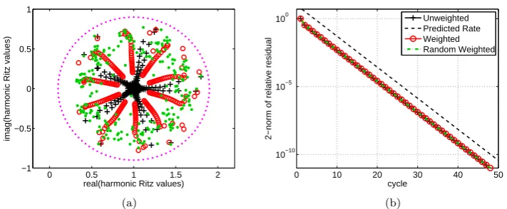
[image:9.595.58.415.105.431.2]0 0.5 1 1.5 2 −1
−0.5 0 0.5 1
real(harmonic Ritz values)
imag(harmonic Ritz values)
(a)
0 10 20 30 40 50 10−10
10−5 100
cycle
2−norm of relative residual
Unweighted Predicted Rate Weighted Random Weighted
(b)
Fig. 2: (a) Harmonic Ritz values for GMRES(5) (black +), WGMRES(5) with (2) (red◦), and WGMRES(5) withDrand (green dots) for a 100×100 matrix
with eigenvalues distributed on the shifted unit circle. The harmonic Ritz val-ues are shown at the end of each of 50 cycles. (b) Relative 2-norm residuals for the considered GMRES(5) variants. (All three convergence curves are visually indistinguishable.)
polynomial is bounded by
qm(z∗)
qm(0)
=
qm(1 +βeπi/N)
qm(0)
=
βmeπim/N −αm (−1)m−αm
≈βm
for sufficiently smallα. This explains why we see convergence with rate β in Figure 2 (b), indicated by the black dashed line, and weighting has essentially no effect on the convergence here.
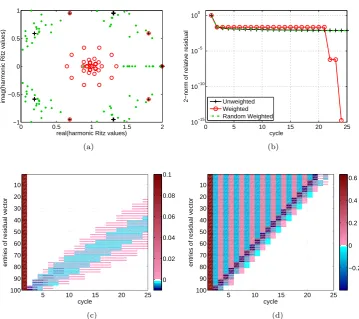
Example 3 (Jordan block) Our next example is an upper triangular Jor-dan block J of size N = 100 with eigenvalue 1. The right-hand side b is a vector of all ones, scaled to unit length. As one can see in Figure 3 (b), the unweighted GMRES(5) method will stagnate except in the first cycle, where a little progress is made. The corresponding harmonic Ritz values reappear at10 points on a circle of radius one around the eigenvalue 1, with the real point θ = 2 being counted twice due to symmetry, see Figure 3 (a). The harmonic Ritz values associated with Essai’s weighted GMRES(5) method move closer towards the eigenvalue1with each cycle. After23cycles, weighted GMRES(5) has found the exact solution ofJx=b. The random weighting matrix Drand
leads to stagnation just as unweighted GMRES(5). As opposed to the previous two examples, the harmonic Ritz values shown in Figure 3 (a) do not explain the convergence curves in Figure 3 (b) for this (highly) nonnormal example.
[image:10.595.54.410.104.251.2] [image:10.595.118.362.378.408.2]entries of the residual vector after each cycle. The special structure of the Jor-dan matrix results in large residual entries being shifted up the vector with each cycle. With unweighted GMRES(5) the residual vector is initially largest in its last entries. This phenomenon is fully described by Theorem 2.1 in [20], which is stated in terms of the transpose of the Jordan block,JT, but is also valid for
J. Some intuition is gained by observing that if S =
0,e1, . . . ,eN−1
is the noncircular shift matrix, thenKm(J,r) =Km(S,r)for any vectorr. It follows that the first two basis vectors,randSrdiffer only in the last component and this affects the weight of the residual. More generally, any two basis vectors SjrandSj+1rdiffer in the(N−j)-th component only. Thus the “support” of
nonzero entries in the residual vector at the end of the first cycle is in the last five components of the residual. At later cycles, this “support” forms a band that gets wider with each cycle, eventually polluting all entries of the residual vector and causing the method to stagnate. WGMRES(5) with Essai’s weight-ing initially has largest entries at the bottom of the residual vector, although the other components also have some weight. Weighted GMRES then “cleans up” the entries of the residual vector which were large in the previous cycle because more weight is placed at those entries. Eventually, this WGMRES(5) variant finds the exact solution in the 24-th cycle.
Note that this Jordan example also explains why the Krylov space and hence the residual at the end of a cycle may depend sensitively on the initial resid-ual for that cycle: instead of working with the matrix J and right-hand side vector bwe could as well run restarted weighted or unweighted GMRES with A = XJ X−1 and eb = Xb, where X = [x1, . . . ,xN] is an arbitrary
invert-ible matrix. Since Km(A,eb) = XKm(J,b), each column of Figure 3 (c) and
(d) can now be interpreted as the components of a residual vector in the basis of generalized eigenvectors of A. If a zero component rj of a residual vector
r = [r1, . . . , rN]T is altered from 0 to > 0, for example by finite precision
arithmetic, then this can cause a change of an eigenvector component in Ar (and the following Krylov subspace vectors) of order kxjk, which can be
ar-bitrarily large depending onkxjk.
0 0.5 1 1.5 2 −1
−0.5 0 0.5 1
real(harmonic Ritz values)
imag(harmonic Ritz values)
(a)
0 5 10 15 20 25 10−15
10−10 10−5 100
cycle
2−norm of relative residual Unweighted Weighted Random Weighted
(b)
5 10 15 20 25 10
20 30 40 50 60 70 80 90 100
cycle
entries of residual vector
0 0.02 0.04 0.06 0.08 0.1
(c)
5 10 15 20 25 10
20 30 40 50 60 70 80 90 100
cycle
entries of residual vector
−0.2 0 0.2 0.4 0.6
(d)
Fig. 3: (a) Harmonic Ritz values for GMRES(5) (black +), WGMRES(5) with (2) (red◦), and WGMRES(5) withDrand(green dots) for a Jordan block with
eigenvalue 1. The harmonic Ritz values are shown at the end of each of the 25 cycles. The eigenvalue at 1 is plotted as an orange dot. (b) Relative 2-norm residuals for the considered GMRES(5) variants. (The convergences curves of WGMRES(5) with Drand and GMRES(5) are visually hard to distinguish.)
(c) Entries of the residual vectors after each cycle of unweighted GMRES(5). (d) Entries of the residual vectors after each cycle of GMRES(5) with Essai’s weighting.
3 The weighted Arnoldi algorithm
[image:12.595.56.416.100.419.2]3.1 Variants of the algorithm
The most straightforward implementation of the weighted Arnoldi algorithm replaces Euclidean inner products in a standard Arnoldi algorithm byD-inner products (see, e.g., [13, 29]). With modified Gram–Schmidt orthogonalization (MGS)2 the j-th iteration requires the computation of j D-inner products
(see Algorithm 1). If D is a diagonal matrix like (2), the inner products can be efficiently implemented as (v◦d)HuorvH(d◦u), where◦ represents the
Hadamard product and d the vector of diagonal elements of D. Each step of Algorithm 1 is more expensive than a step of the Arnoldi algorithm in the Euclidean inner product because of theD-inner products and D-norms. However, Algorithm 1 can be used with a preconditioner in a straightforward manner.
As an alternative to computing D-inner products at each step of the weighted Arnoldi algorithm, we can apply the Arnoldi algorithm in the Eu-clidean inner product to the transformed matrixAe=D
1 2AD−
1
2 and starting
vectorer=D12r. Doing so gives matricesVem andHemthat satisfy
e
AVem=Vem+1Hem, (9)
where Hem is an upper Hessenberg matrix, VemHVem = Im, and the columns
of Vem form a basis of Km(A,e er). Premultiplying both sides of (9) by D−
1 2
gives the Arnoldi decompositionAVm=Vm+1Hm, whereVm=D−
1
2Vem and
Hm =Hem. The columns of Vm areD-orthonormal and spanKm(A,r) since
the columns ofVemspanKm(D
1 2AD−
1 2, D
1 2r).
The resulting algorithm with MGS orthogonalization is given in Algo-rithm 2. We note that a similar orthogonalization strategy was considered in the context of rounding error analysis in [26]. Additionally, Heyouni and Es-sai [17] considered the use of matrix square roots for enforcingD-orthogonality when solving systems with multiple right-hand sides, although they still com-putedD-inner products at each iteration of their weighted Arnoldi algorithm. It does not seem feasible to use Algorithm 2 in this form with a precondi-tionerP. However, a (right) preconditioner can be incorporated by replacing the two-sided scaling forAein line 1 of this algorithm with a one-sided
scal-ing Ae1 = D
1
2A, and line 5 with w =Ae1P−1D−1/2
e
vk (and similarly for left
preconditioning).
In the remainder of this manuscript, we use Algorithms 1 and 2 to refer to both the weighted Arnoldi variants and the corresponding WGMRES(m) methods. The meaning will be clear from the context. Although it is easiest
Variants of the weighted Arnoldi algorithm:
Inputs: Matrix A ∈ CN×N, diagonal positive definite weight matrix D ∈ CN×N, vectorr∈CN, number of Arnoldi iterationsm
Outputs:D-orthonormal Arnoldi vectors{v1. . . ,vm}ofKm(A,r) and upper
Hessenberg matrixHm= [hij]∈C(m+1)×m
Algorithm 1: Explicit D-inner products and MGS or-thogonalization
1 Ae=D
1 2AD−
1 2
2 w=D12r
1 v1=r/krkD
2 fork= 1,2, . . . , mdo 3 w=Avk
4 forj= 1,2, . . . , k do 5 hjk=v∗jDw 6 w=w−vjhjk 7 end
8 hk+1,k=kwkD 9 if hk+1,k= 0then 10 Stop
11 end
12 vk+1=w/hk+1,k 13 end
14 [v1, . . . ,vm] =D−
1
2[ev1, . . . ,evm]
Algorithm 2: Implicit D-inner products and MGS or-thogonalization
1 Ae=D
1 2AD−
1 2
2 w=D12r 3
e
v1=w/kwk2
4 fork= 1,2, . . . , mdo 5 w=Aeevk
6 forj= 1,2, . . . , k do 7 hjk=ve∗jw 8 w=w−evjhjk 9 end
10 hk+1,k=kwk2 11 if hk+1,k= 0then 12 Stop
13 end
14 evk+1=w/hk+1,k 15 end
16 [v1, . . . ,vm] =D−
1
2[ev1, . . . ,evm]
to monitorkr(k)k
D(k) in WGMRES(m), we measure instead the reduction of
the residualkr(k)k2for fair comparison with GMRES(m).
3.2 Operation counts
In both variants of the Arnoldi algorithm discussed here, the number of matrix-vector products is m, and their computation requires 2m×Nnz arithmetic operations, whereNnzis the number of nonzero elements in the matrixAorA,e
respectively. Furthermore, the successive orthogonalization ofmKrylov basis vectors requires m(m+ 1)/2 inner products and vector updates of the form w =w−vjhjk. One such vector update requires 2N arithmetic operations.
Computing a single inner product requires 2N or 3N arithmetic operations in the unweighted or weighted case, respectively. The row and column3 scaling 3 As pointed out by one of the referees, the column scaling in Algorithm 2 can be elim-inated, at the expense of storingmadditional vectors, by computing each Arnoldi vector
vk=D−12evkas soon asevkis available. In this case,w=D −1
Table 1: Operation counts for a cycle of Algorithms 1 and 2 and GMRES-DR.
Algorithm 1 2m×Nnz+52N m2
Algorithm 2 2m×Nnz+N(2m2+m+ 2p+ 3)
GMRES-DR 2m×Nnz+N(2m2+ 2m`)
of the matrix A to form Ae and vector r to form er in Algorithm 2 requires
3N+2×Nnzoperations, counting the computation of a square root or a division as a single arithmetic operation. Algorithm 2 also requiresN mmultiplications to scale the basis vectors at the end of each cycle.
In Section 4 we will compare different variants of WGMRES(m) with GMRES-DR(m, `) [23] on various numerical examples, but it easy to discuss the computational cost theoretically as well. In each cycle, GMRES-DR(m, `) augments the Krylov basis computed by GMRES(m) with the Schur vectors corresponding to the ` smallest harmonic Ritz values. These Schur vectors, and the initial residual of the new cycle k, form the columns of a matrix P`+1∈C(m+1)×(`+1), from which the first`+ 1 basis vectors of the new cycle
are obtained viaV`+1(k)=Vm+1(k−1)P`+1.The dense matrix-matrix multiplication
to obtainV`+1(k) requires 2N(m+ 1)(`+ 1) arithmetic operations and so domi-nates the cost of augmenting the Krylov basis. The remaining columns ofV`+m(k) are then computed by the Arnoldi algorithm. Depending on the restart length mand the number of Schur vectors`, one cycle of GMRES-DR(m, `) may be more costly than a cycle of WGMRES(m).
We summarize the operation counts for a single cycle of Algorithms 1 and 2 and GMRES-DR in Table 1, lettingp=Nnz/N be the average number of nonzeros per row. Although the performance of each algorithm is machine dependent Algorithm 2, for which the cost of the weighted inner product is independent of the restart length, can become more efficient than Algorithm 1 when 2p < m2/2−m−3, i.e., when the average number of nonzeros per
row is sufficiently small and the restart length is sufficiently large (or when reorthogonalization is used).
4 Numerical experiments
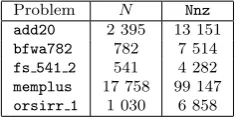
Table 2: Size of, and number of nonzeros in, the matrices in Essai’s problems.
Problem N Nnz
add20 2 395 13 151 bfwa782 782 7 514 fs 541 2 541 4 282 memplus 17 758 99 147 orsirr 1 1 030 6 858
the storage needs and orthogonalization costs of these algorithms are com-parable. The last example compares Algorithm 1, unweighted GMRES(m), GMRES-DR(m, `) and BICGSTAB over a large set of right-preconditioned test problems that is described below.
In the first example the right-hand side b is a random vector, to be con-sistent with Essai, while in the second beither comes with the matrix, or is generated randomly. We setx(0) =0and stop a method whenkr(k)
j k2/kbk2
falls below 10−10 or when 100 cycles are performed; the latter case is denoted
by ‘—’. Iteration counts are given in the form itout(itin), where itout is the
number of cycles anditin is the number of steps in the last cycle. In our
no-tation GMRES-DR(m, `) augments a Krylov subspace of dimensionmwith` approximate Schur vectors so that that all GMRES variants require exactly mmatrix-vector products with Ain a cycle. We choose`= 5,10 so that the cost of augmenting with Schur vectors is not too high.
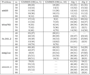
Example 4 (Essai problems) The first example comprises the five prob-lems considered by Essai [13] (see Table 2 for problem details). We see from Table 3 that GMRES-DR converges in fewer cycles than WGMRES(m) for add20, bfwa782 and fs 541 2. Indeed, for fs 541 2 WGMRES with m = 40,80 fails to converge within 100 cycles. For memplus, on the other hand, WGMRES(m) requires fewer cycles than GMRES-DR(m,5), except whenm= 80, but more than GMRES-DR(m,10), except when m = 50. When applied to orsirr 1, WGMRES(m) converges faster than GMRES-DR(m,5) when m= 40,50,80, while GMRES-DR(m,10) does not converge within 100 cycles for any m.
Essai found that for these problems WGMRES(m) consistently outper-formed GMRES(m). However, WGMRES does not always perform as well as GMRES-DR, which also alters the harmonic Ritz values via deflation. Never-theless, WGMRES is still competitive for problems likememplusandorsirr 1, for which GMRES-DR can stagnate or converge slowly if the number of ap-proximate Schur vectors ` in not well chosen. We note that in practice the optimal`is usually unknown, while WGMRES has no parameters to choose.
Table 3: Number of cycles for Essai’s problems.
Problem m GMRES-DR(m,5) GMRES-DR(m,10) Alg 1 Alg 2
add20
40 20(23) 18(20) 21(35) 21(35)
50 14(44) 14(5) 15(32) 15(32)
60 11(49) 11(26) 12(43) 12(43)
70 10(36) 10(15) 11(12) 11(12)
80 9(12) 8(69) 10(5) 10(5)
bfwa782
40 17(13) 9(2) 65(34) 69(24)
50 11(34) 7(23) 34(26) 34(27)
60 8(33) 6(18) 28(58) 28(58)
70 7(42) 5(36) 22(5) 22(5)
80 6(46) 4(70) 14(56) 14(56)
fs 541 2
40 35(27) 29(21) — —
50 22(18) 20(49) 23(47) 23(42)
60 18(49) 16(53) 25(60) 25(60)
70 13(48) 12(62) 21(65) 22(9)
80 10(78) 9(76) — —
memplus
40 60(40) 48(32) 50(24) 54(29)
50 42(27) 33(41) 35(33) 33(2)
60 33(9) 25(54) 28(31) 27(60)
70 25(51) 21(50) 26(26) 26(37)
80 20(51) 18(2) 20(49) 20(9)
orsirr 1
40 70(9) — 61(35) 58(2)
50 55(13) — 46(46) 48(11)
60 34(55) — 35(41) 34(32)
70 25(12) — 28(39) 28(18)
80 — — 22(32) 23(8)
Example 5 (performance profile) To get a general idea of whether WGM-RES is a practical method when preconditioners are used, we compare GMWGM-RES and Algorithm 1, as well as GMRES-DR and BICGSTAB, on a large num-ber of problems from the University of Florida Sparse Matrix Collection. In contrast to Cao and Yu [6] we use right preconditioning which minimizes the residual.
Our method of comparison is as follows. We first retrieve the 220 non-symmetric matrices A of sizes between 104 and106 with at most 15 nonzero
elements per row on average. We then apply sparse reverse Cuthill–McKee re-ordering as implemented in Matlab’s symrcm. Next we scale the columns ofA to have unit Euclidean norm, followed by a scaling of the rows of A to unit norm. Our aim is to compute an ILU preconditioner with thresholding and pivoting via Matlab’s ilu. For stability reasons we compute an ILU factor-ization of A+σI, where σ = 10−12 if all diagonal elements of A are zero,
or σ= 10−12max{|aii|} if some but not all diagonal elements a
ii of A zero,
or σ= 0 otherwise. This procedure follows recommendations in [7]. We suc-cessively use a drop tolerance of 10−3,10−4, . . . ,10−8, and stop when the U
factor of the factorization has a condition number below 1015, so that it can
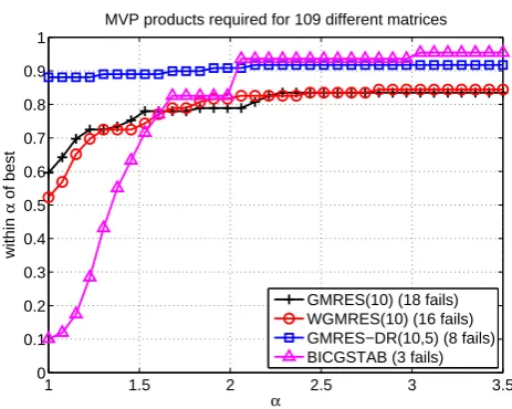
We now run the Krylov methods GMRES(10), WGMRES(10), GMRES-DR(10,5), BICGSTAB on the test matrices. A method is marked as failed if more than 50 restart cycles or 250 BICGSTAB iterations are required to obtain a relative residual norm of10−8. Note that in our notation GMRES-DR(10,5) requires10matrix-vector products (MVP) per cycle, exactly like GMRES(10) and WGMRES(10), and BICGSTAB requires 2 MVP per iteration, so that the maximal number of MVP is 500 for all methods. If all methods fail on a matrix it is excluded from the test. Since the collection contains many singular matrices, related to eigenvalue or least-squares problems, only 109 out of the 220 retrieved matrices are finally included in our test.
The performance profile in Figure 4 allows us to compare the number of MVP needed for each method to converge across all test problems. More specif-ically, if for each linear system the performance ratio measures the number of MVP for thek-th method to converge to the number of MVP for the best per-forming method to converge, then the functionfk(α) measures the fraction of
problems in the test set for which the performance ratio of method k is less than or equal to α. Thus, α = 1 shows the fraction of problems for which the k-th method requires the fewest MVP of all methods. Also, limα→∞fk(α)
indicates the number of failures.
It is somewhat disappointing that WGMRES(10) is generally outperformed by GMRES(10). We note that GMRES(10) and WGMRES(10) fail on at least 16 matrices from our test set; this failure rate is considerably higher than for GMRES-DR and BICGSTAB. Overall, GMRES-DR(10,5) requires fewest MVP in general, and thereby outperforms all other methods under consider-ation. It is, however, less robust than BICGSTAB, the latter of which fails for 3 matrices only but typically requires the most MVP. To summarize, we believe that WGMRES should not be used in combination with preconditioners, although we are aware that for some examples it may perform satisfactorily.
5 Conclusions
The weighted GMRES variant presented by Essai has recently gained interest for solving linear systems. This method is justified by a heuristic that empha-sizes large residual components via a weighted inner product. With the help of simple model problems we have given insight into how weighting affects the distribution of harmonic Ritz values, or how it affects entries in the residual vector after each cycle. For example, in one case where the harmonic Ritz val-ues appeared in cyclic pairs on the spectral interval of a matrix, weighting had the effect of “randomizing” these harmonic Ritz values, thereby covering the spectral interval more evenly. This led to an improved convergence of WGM-RES compared to the linear convergence observed for GMWGM-RES on the same example.
1 1.5 2 2.5 3 3.5 0
0.1 0.2 0.3 0.4 0.5 0.6 0.7 0.8 0.9 1
α
within
α
of best
MVP products required for 109 different matrices
[image:19.595.120.352.87.272.2]GMRES(10) (18 fails) WGMRES(10) (16 fails) GMRES−DR(10,5) (8 fails) BICGSTAB (3 fails)
Fig. 4: Performance profile of matrix vector products required by various Krylov methods applied to 109 matrices from the University of Florida Sparse Matrix Collection with an ILU preconditioner.
When applied to unpreconditioned problems, WGMRES(m) can outperform GMRES(m). However, a test run with many matrices from the University of Florida Sparse Matrix Collection revealed, similarly to observations in [6], that weighted GMRES is typically outperformed by GMRES if a precon-ditioner is used. In addition, we compared these methods with other state-of-the-art Krylov methods like GMRES-DR (GMRES with deflated restart-ing) and BICGSTAB. GMRES-DR required fewest matrix-vector products, whereas BICGSTAB appeared to be the most robust method in our test, at the cost of requiring the most matrix-vector products. One advantage of WGMRES(m) over GMRES-DR(m, `) is that there is no parameter` to be chosen.
We find that, although weighted GMRES may outperform unweighted GM-RES for some examples, in general this method is not competitive with other Krylov subspace methods like BICGSTAB or deflated GMRES, in particular when preconditioners are used.
Acknowledgements We are grateful to Andy Wathen and the anonymous referees for
their valuable comments and suggestions.
References
2. Akaike, H.: On a successive transformation of probability distribution and its application to the analysis of the optimum gradient method. Ann. Inst. Statist. Math.11, 1–16 (1959)
3. Arioli, M., Pt´ak, V., Strakoˇs, Z.: Krylov sequences of maximal length and convergence of GMRES. BIT38, 636–643 (1998)
4. Baker, A.H., Jessup, E.R., Manteuffel, T.: A technique for accelerating the convergence of restarted GMRES. SIAM J. Matrix Anal. Appl.26, 962–984 (2005)
5. Brown, P.: A theoretical comparison of the Arnoldi and GMRES algorithms. SIAM J. Sci. Stat. Comput.12, 58–78 (1991)
6. Cao, Z.H., Yu, X.Y.: A note on weighted FOM and GMRES for solving nonsymmetric linear systems. Appl. Math. Comput.151, 719–727 (2004)
7. Chow, E., Saad, Y.: Experimental study of ILU preconditioners for indefininte matrices. J. Comput. Appl. Math.86, 387–414 (1997)
8. Davis, T.A., Hu, Y.: The University of Florida Sparse Matrix Collection. ACM Trans. Math. Softw.38, 1:1–1:25 (2011)
9. Duintjer Tebbens, J., Meurant, G.: Any Ritz value behavior is possible for Arnoldi and for GMRES with any convergence curve. SIAM J. Matrix Anal. Appl.33(3), 958–978 (2012)
10. Eiermann, M., Ernst, O.G.: Geometric aspects in the theory of Krylov subspace meth-ods. Acta Numer.10, 251–312 (2001)
11. Eiermann, M., Ernst, O.G., Schneider, O.: Analysis of acceleration strategies for restarted minimal residual methods. J. Comput. Appl. Math.123, 261–292 (2000) 12. Embree, M.: The tortoise and the hare restart GMRES. SIAM Rev.45, 259–266 (2003) 13. Essai, A.: Weighted FOM and GMRES for solving nonsymmetric linear systems.
Nu-mer. Algorithms18, 277–292 (1998)
14. Forsythe, G.E., Motzkin, T.S.: Asymptotic properties of the optimum gradient method (abstract). Bull. Amer. Math. Soc.57, 183 (1951)
15. Goossens, S., Roose, D.: Ritz and harmonic Ritz values and the convergence of FOM and GMRES. Numer. Linear Algebra Appl.6, 281–293 (1997)
16. Greenbaum, A., Pt´ak, V., Strakoˇs, Z.: Any nonincreasing convergence curve is possible for GMRES. SIAM J. Matrix Anal. Appl.17, 465–469 (1996)
17. Heyouni, M., Essai, A.: Matrix Krylov subspace methods for linear systems with multiple right-hand sides. Numer. Algorithms40, 137–156 (2005)
18. Horn, R.A., Johnson, C.R.: Matrix Analysis. Cambridge University Press, New York, NY (1990)
19. Jing, Y.F., Huang, T.Z.: Restarted weighted full orthogonalization method for shifted linear systems. Comput. Math. Appl.57, 1583–1591 (2009)
20. Liesen, J., Strakoˇs, Z.: Convergence of GMRES for tridiagonal Toeplitz matrices. SIAM J. Matrix Anal. Appl.26, 233–251 (2004)
21. Meijerink, J.A., van der Vorst, H.A.: An iterative solution method for linear systems of which the coefficient matrix is a symmetricM-matrix. Math. Comput.31, 148–162 (1977)
22. Morgan, R.B.: A restarted GMRES method augmented with eigenvectors. SIAM J. Ma-trix Anal. Appl.16, 1154–1171 (1995)
23. Morgan, R.B.: GMRES with deflated restarting. SIAM J. Sci. Comput.24, 20–37 (2002) 24. Najafi, H.S., Zareamoghaddam, H.: A new computational GMRES method.
Appl. Math. Comput.199, 527–534 (2008)
25. Niu, Q., Lu, L., Zhou, J.: Accelerate weighted GMRES by augmenting error approxi-mations. Int. J. Comput. Math.87, 2101–2112 (2010)
26. Rozloˇzn´ık, M., T˚uma, M., Smoktunowicz, A., Kopal, J.: Numerical stability of orthog-onalization methods with a non-standard inner product. BIT Numer. Math.52, 1035– 1058 (2012)
27. Saad, Y.: Analysis of augmented Krylov subspace methods. SIAM J. Matrix Anal. Appl. 18, 435–449 (1997)
28. Saad, Y., Schultz, M.H.: GMRES: a generalized minimal residual algorithm for solving nonsymmetric linear systems. SIAM J. Sci. Stat. Comput.7, 856–869 (1986)
30. Simoncini, V., Szyld, D.B.: On the occurence of superlinear convergence of exact and inexact Krylov subspace methods. SIAM Rev.47, 247–272 (2005)
31. Vecharynski, E., Langou, J.: The cycle-convergence of restarted GMRES for normal matrices is sublinear. SIAM J. Sci. Comput.32, 186–196 (2010)
32. Vecharynski, E., Langou, J.: Any admissible cycle-convergence behavior is possible for restarted GMRES at its initial cycles. Numer. Linear Algebra Appl.18, 499–511 (2011) 33. Wang, Z., Qi, J., Liu, C., Li, Y.: Weighted harmonic Arnoldi method for large interior
eigenproblems. World Acad. Sci. Eng. Technol.56, 1476–1479 (2011)
34. Zavorin, I., O’Leary, D.P., Elman, H.: Complete stagnation of GMRES. Linear Algebra Appl.367, 165–183 (2003)
35. Zhong, B., Morgan, R.B.: Complementary cycles of restarted GMRES. Numer. Linear Algebra Appl.15, 559–571 (2008)
36. Zhong, B.J.: A product hybrid GMRES algorithm for nonsymmetric linear systems. J. Comput. Math.23, 83–92 (2005)
![Fig. 1: (a) Harmonic Ritz values for GMRES(5) (black +), WGMRES(5) with(2) (red ◦), and WGMRES(5) with Drand (green dots) for a diagonal matrixwith equispaced eigenvalues on [1, 100]](https://thumb-us.123doks.com/thumbv2/123dok_us/1635890.116907/9.595.58.415.105.431/harmonic-values-wgmres-wgmres-diagonal-matrixwith-equispaced-eigenvalues.webp)