A Systematic Comparison of Music Similarity Adaptation Approaches

City, University of London Institutional Repository

Citation

:

Wolff, D., Stober, S., Nürnberger, A. and Weyde, T. (2012). A Systematic

Comparison of Music Similarity Adaptation Approaches. Paper presented at the 13th

International Society for Music Information Retrieval Conference (ISMIR 2012), 8 - 12 Oct

2012, Porto, Portugal.

This is the unspecified version of the paper.

This version of the publication may differ from the final published

version.

Permanent repository link: http://openaccess.city.ac.uk/2963/

Link to published version

:

Copyright and reuse:

City Research Online aims to make research

outputs of City, University of London available to a wider audience.

Copyright and Moral Rights remain with the author(s) and/or copyright

holders. URLs from City Research Online may be freely distributed and

linked to.

City Research Online:

http://openaccess.city.ac.uk/

publications@city.ac.uk

A SYSTEMATIC COMPARISON OF

MUSIC SIMILARITY ADAPTATION APPROACHES

Daniel Wolff

, Tillman Weyde

MIRG, School of Informatics

City University London, UK

daniel.wolff.1@city.ac.uk

Sebastian Stober

, Andreas N ¨urnberger

Data & Knowledge Engineering Group

Otto-von-Guericke-Universit¨at Magdeburg, DE

stober@ovgu.de

ABSTRACT

In order to support individual user perspectives and differ-ent retrieval tasks, music similarity can no longer be con-sidered as a static element of Music Information Retrieval (MIR) systems. Various approaches have been proposed recently that allow dynamic adaptation of music similarity measures. This paper provides a systematic comparison of algorithms for metric learning and higher-level facet dis-tance weighting on theMagnaTagATunedataset. A cross-validation variant taking into account clip availability is presented. Applied on user generated similarity data, its effect on adaptation performance is analyzed. Special at-tention is paid to the amount of training data necessary for making similarity predictions on unknown data, the num-ber of model parameters and the amount of information available about the music itself.

1. INTRODUCTION

Musical similarity is a central issue in MIR and the key to many applications. In the classical retrieval scenario, similarity is used as an estimate for relevance to rank a list of songs or melodies. Further applications comprise the sorting and organization of music collections by group-ing similar music clips or generatgroup-ing maps for a collection overview. Finally, music recommender systems that fol-low the popular “find me more like. . . ”-idea often employ a similarity-based strategy as well. However, music sim-ilarity is not a simple concept. In fact there exist various frameworks within musicology, psychology, and cognitive science. For a comparison of music clips, many interre-lated features and facets can be considered. Their individ-ual importance and how they should be combined depend very much on the user and her or his specific retrieval task. Users of MIR systems may have various (musical) back-grounds and experience music in different ways. Conse-quently, when comparing musical clips with each other, opinions may diverge. Apart from considering individual

*The two leading authors contributed equally to this work.

Permission to make digital or hard copies of all or part of this work for personal or classroom use is granted without fee provided that copies are not made or distributed for profit or commercial advantage and that copies bear this notice and the full citation on the first page.

c

2012 International Society for Music Information Retrieval.

users or user groups, similarity measures also should be tailored to their specific retrieval task to improve the per-formance of the retrieval system. For instance, when look-ing for cover versions of a song, the timbre may be less interesting than the lyrics. Various machine learning ap-proaches have recently been proposed for adapting a music similarity measure for a specific purpose. They are briefly reviewed in Section 2. For a systematic comparison of these approaches, a benchmark experiment based on the

MagnaTagATunedataset has been designed, which is de-scribed inSection 3. Section 4discusses the results of the comparison andSection 5finally draws conclusions.

2. ADAPTATION APPROACHES

The approaches covered in this paper focus on learning a distance measure, which (from a mathematical perspec-tive) can be considered as a dual concept to similarity. The learning process is guided by so-called relative distance constraints. A relative distance constraint(s, a, b)demands that the objectais closer to the seed objectsthan objectb, i.e.,

d(s, a)< d(s, b) (1) Such constraints can be seen as atomic bits of information fed to the adaptation algorithm. They can be derived from a variety of higher-level application-dependent constraints. For instance, in the context of interactive clustering, as-signing a song sto a target cluster with the prototypect

can be interpreted by the following set of relative distance constraints as proposed by Stober et al. [11]:

d(s, ct)< d(s, c) ∀c∈C\ {ct} (2)

In the following, the two general approaches covered in this comparison are briefly reviewed.

2.1 Linear Combinations of Facet Distances

Stober et al. model the distanced(a, b)between two songs as weighted sum offacet distancesδf1(a, b), . . . , δfl(a, b):

d(a, b) = l X

i=1

wiδfi(a, b) (3)

Each facet distance refers to an objective comparison of two music clips with respect to a single facet of music in-formation such as melody, timbre, or rhythm. Here, the facet weights w1, . . . , wl ∈ R+ serve as parameters of

the distance measure that allow to adapt the importance of each facet to a specific user or retrieval task. These weights obviously have to be non-negative so that the aggregated distance cannot decrease where a single facet distance in-creases. Furthermore, the sum of the weights should be constant such as l

X

i=1

wi=l (4)

to avoid arbitrarily large distance values.

The small number of parameters somewhat limits the expressivity of the distance model. However, at the same time, the weights can easily be understood and directly ma-nipulated by the user. Stober et al. argue that this design choice specifically addresses the users’ desire to remain in control and not to be patronized by an intelligent sys-tem that “knows better”. In [11], they describe various ap-plications and respective adaptation algorithms which they evaluate and compare in [12] using the MagnaTagATune

dataset. Three of these approaches are covered by the com-parison in this paper.

2.1.1 Gradient Descent

Here, if a constraint is violated by the current distance mea-sure, the weighting is updated by trying to maximize

obj(s, a, b) = l X

i=1

wi(δfi(s, b)−δfi(s, a)) (5)

which can be directly derived fromEquation 1. This leads to the following update rule for the individual weights:

wi=wi+η∆wi, with (6) ∆wi=

∂obj(s, a, b)

∂wi

=δfi(s, b)−δfi(s, a) (7)

where the learning rateηdefines the step width of each it-eration. As in [12], the optimization process is restarted 50 times with random initialization and the best result is cho-sen to reduce the risk of getting stuck in a local optimum.

2.1.2 Quadratic Programming

Of the various quadratic programming approaches covered in [12], only the one minimizing the quadratic slack is con-sidered here because it was the best performing one in the original comparison. In this approach, an individual slack variable is used for each constraint, which allows viola-tions. As optimization objective, the sum of the squared slack values has to be minimized.

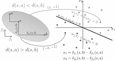
relative distance constraints linear classification problem

Figure 1. Transformation of a relative distance constraint for linear combination models into two training instances of the corresponding binary classification problem as de-scribed by Cheng et al. [3].

2.1.3 Linear Support Vector Machine (LibLinear)

The third approach takes a very different perspective. As described by Cheng et al. [3], the learning task can be re-formulated as a binary classification problem, which opens the possibility to apply a wide range of sophisticated clas-sification techniques such as (linear) Support Vector Ma-chines (SVMs). Figure 1illustrates this idea to rewrite each relative distance constraintd(s, a)< d(s, b)as

m X

i=1

wi(δfi(s, b)−δfi(s, a)) = m X

i=1

wixi=wTx>0 (8)

wherexiis thedistance differencewith respect to facetfi.

The positive training example(x,+1)then represents the satisfied constraint whereas the negative example(−x,−1)

represents its violation (i.e., inverting the relation sign). For these training examples, the normal vector of the hy-perplane that separates the positive and negative instances contains the adapted facet weights. As in [12], the Lib-Linearlibrary is used here, which finds a stable separating hyperplane but still suffers from the so far unresolved prob-lem that the non-negativity of the facet weights cannot be enforced.

2.2 Metric Learning

Alternative approaches to weighting predefined facet dis-tance measures include direct manipulation of parametrized vector distance measures. All features are concatenated to a single combined feature vector per clip. We model a clip’s feature vector by g(a) : N 7→ RN. This

corre-sponds to assigning a single facet to each feature dimen-sion. Frequently, the mathematical form of Mahalanobis metrics is used to specify a parametrized vector distance measure. In contrast to the approaches described in the pre-vious section, adaptation is performed in the (combined) feature space itself: Given two feature vectorsa = g(a),

b=g(b)∈RN, the family of Mahalanobis distance

mea-sures can be expressed by

dW(a,b) =

q

(a−b)T_{W(a−b), (9)}

whereW∈RN×N is a positive semidefinite matrix,

Euclidean metric, Mahalanobis metrics allow for linear trans-formation of the feature space when accessing distance. An important property of this approach is that the number of adjustable parameters directly depends on the dimen-sionality N of the feature space. As this number grows quadratically withN, many approaches restrict training to theNparameters of a diagonal matrixW, only permitting a weighting of the individual feature dimensions.

2.2.1 Linear Support Vector Machine (SVMLight)

The SVM approach explained in Section 2.1.3 has been shown as well suited to learning a Mahalanobis distance measure: Schultz et al. [10] adapted a weighted kernelized metric towards relative distance constraints. We follow the approach of Wolff et al. [13], where a linear kernel is used. This simplifies the approach of Schultz et al. to learning a diagonally restricted Mahalanobis distance (Equation 9).

Like the SVM for the facet distances, a large margin classifier is optimized to the distance constraints. Here, for each constraint(s, a, b), we replace the facetdistance differencevectorxinEquation 8with the difference of the pointwise squared1 feature difference vectorsx = (s−

b)2−(s−a)2.

Given the vectorw=diag(W),wi≥0and slack

vari-ablesξ(s,a,b)≥0, optimization is performed as follows:

min

w,ξ

1 2w

T_w+c· X

(s,a,b)

ξ(s,a,b) (10)

s.t.∀(s, a, b) wTx(s,a,b)≥1−ξ(s,a,b)

Here,cdetermines a trade-off between regularization and the enforcement of constraints. For the experiments below, the SVMlightframework2 is used to optimize the weights

wi. As forLibLinear,wi≥0cannot be guaranteed.

2.2.2 Metric Learning to Rank

McFee et al. [9] developed an algorithm for learning a Ma-halanobis distance from rankings.3 Using the constrained regularization of Structural SVM, the matrix Wis opti-mized to an input of clip rankings and their feature vectors. Given a relative distance constraint(s, a, b)(seeEquation 1), the corresponding ranking assigns a higher ranking score toathan tob, when querying clips. For a setXof training query feature vectorsq∈X ⊂RN and associated training

rankingsy_q∗, Metric Learning to Rank (MLR) minimizes

min

W,ξ tr(W

T_{W) +c}1

n

X

q∈X

ξq, (11)

s.t. ∀q∈X, ∀y∈Y \ {y∗_q}:

HW q, yq∗

≥HW(q, y) + ∆(yq∗, y)−ξq,

withWi,j ≥ 0 andξq ≥ 0. Here, the matrixWis

reg-ularized using the trace. Optimization is subject to the constraints creating a minimal slack penalty of ξq. c

de-termines the trade-off between regularization and the slack penalty for the constraints below. HW(q, y)4 assigns a

1_(a2₎

i:= (ai)2

2_{http://svmlight.joachims.org/}

3_{http://cseweb.ucsd.edu/˜bmcfee/code/mlr/}

4_{For simplification, HW(q, y) substitutes the Frobenius product} hW, ψ(q, y)i_Fin [9].

score to the validity of rankingy given the queryqwith regard to the Mahalanobis matrixW. This enforces W

to fulfill the training rankingsy∗_q. The additional ranking-loss term∆(y_q∗, y)assures a margin between the scores of given training rankingsy∗q and incorrect rankingsy. The

method is kept efficient by selecting only a few possible alternative rankingsy ∈Y for comparison with the train-ing ranktrain-ings: A separation oracle is used for predicttrain-ing the worst violated constraints (see [6]). In our experiments, an MLR variantDMLRrestrictsWto a diagonal shape.

3. EXPERIMENT DESIGN

3.1 TheMagnaTagATuneDataset

MagnaTagATuneis a dataset combining mp3 audio, acous-tic feature data, user votings for music similarity, and tag data for a set of 25863 clips of about 30 seconds taken from 5405 songs provided by the Magnatune5 _{label. The}

bun-dled acoustic features have been extracted using version 1.0 of theEchoNest API6. The tag and similarity data has been collected using the TagATune game [7]. TagATune is a typical instance of an online “Game With A Purpose”. While users are playing the game mainly for recreational purposes, they annotate the presented music clips. The tag data is collected during the main mode of the game, where two players have to agree on whether they listen to identi-cal clips. Their communication is saved as tag data. The bonus mode of the game involves a typical odd one out survey asking two players to independently select the same outlier out of three clips presented to them. The triplets of clips presented to them vary widely in genre, containing material from ambient and electronica, classical, alterna-tive, and rock.

3.2 Similarity Data

The comparative similarity data inMagnaTagATunecan be represented in a constraint multigraph with pairs of clips as nodes [8, 12]. The vote for an outlierkin the clip triplet

(i, j, k)is transformed into two relative distance constraints:

(i, j, k)and(j, i, k). Each constraint(s, a, b)is represented by an edge from the clip pair(s, a)to(s, b). This results in 15300 edges of which 1598 are unique. In order to adapt similarity measures to this data, the multigraph has to be acyclic, as cycles correspond to inconsistencies in the similarity data. TheMagnaTagATunesimilarity data only contains cycles of length 2, corresponding to contradictive user statements regarding the same triplet. In order to re-move these cycles, the contradicting multigraph edge num-bers are consolidated by subtracting the number of edges connecting the same vertices in opposite directions. The remaining 6898 edges corresponding to 860 unique rela-tive distance constraints constitute the similarity data we work with.7

5_{http://magnatune.com/}

6_{http://developer.echonest.com/}

7_{In [12], the authors report that the number of consistent constraints is}

3.3 Data Partitioning

In order to assess the training performance of the approaches described in Section 2, we compare two cross-validation variants to specify independent test and training sets.

A straightforward method, randomly sampling the con-straints into cross-validation bins and therefore into combi-nations of test and training sets has been used on the dataset before by Wolff et al. [13]. We use this standard method (sampling A) to perform 10-fold cross validation, sampling the data into non-overlapping test and training sets of 86 and 774 constraints respectively

For the second sampling, it is considered that two con-straints were derived from each user voting, as such are related to the same clips. Assigning one of such two con-straints to training and the remaining one to a test set might introduce bias by referring to common information. In our second validation approach, (sampling B) it is assured that the test and training sets also perfectly separate on the clip set. The 860 edges of the MagnaTagATune similar-ity multigraph connect 337 components of three vertices each. These correspond to the initial setup of clip triplets presented to the players during theTagATunegame.

As the removal of one clip causes the loss of all similar-ity information (maximally 3 constraints) within its triplet, the sampling of the test data is based on the triplets rather than the constraints. On the 337 triplets, we use 10-fold cross validation for dividing these into bins of 33 or 34 triplets. Due to the varying number of 2-3 constraints per triplet, the training set sizes vary from 770-779 constraints, leaving the test sets at 81-90 constraints.

For evaluation of generalization and general performance trends, the training sets are analyzed in an expanding sub-set manner. We start with individual training sub-sets of ei-ther 13 constraints (sampling A) or 5 triplets (sampling B), corresponding to 11-15 constraints. The size of the train-ing sets is then increased exponentially, includtrain-ing all the smaller training sets’ constraints in the larger ones. Con-straints remaining unused for each of the smaller training set sizes are used for further validation, and referred to as

unused training constraints. For both sampling methods, all test and training sets are fixed, and referred to as sam-pling Aandsampling B.

3.4 Features and Facets

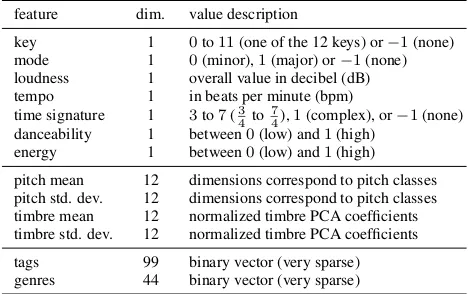
As features, we use those defined in [12] plus the genre features used by Wolff et al. [13]. This results in the set of features shown inTable 1.

Of the 7 global features, “danceability” and “energy” were not contained in the original clip analysis information of the dataset but have become available with a newer ver-sion of theEchoNest API. Furthermore, the segment-based features describing pitch (“chroma”) and timbre have been aggregated (per dimension) resulting in 12-dimensional vec-tors with the mean and standard deviation values. This has been done according to the approach described in [4] for the same dataset. The 99 tags were derived from annota-tions collected through theTagATunegame [7] by applying

feature dim. value description

key 1 0to11(one of the 12 keys) or−1(none) mode 1 0(minor),1(major) or−1(none) loudness 1 overall value in decibel (dB) tempo 1 in beats per minute (bpm)

time signature 1 3to7(3₄ to7₄),1(complex), or−1(none) danceability 1 between0(low) and1(high)

energy 1 between0(low) and1(high) pitch mean 12 dimensions correspond to pitch classes pitch std. dev. 12 dimensions correspond to pitch classes timbre mean 12 normalized timbre PCA coefficients timbre std. dev. 12 normalized timbre PCA coefficients tags 99 binary vector (very sparse) genres 44 binary vector (very sparse)

Table 1. Features for theMagnaTagATunedataset. Top rows: Globally extractedEchoNestfeatures. Middle rows: Aggregation ofEchoNestfeatures extracted per segment. Bottom row: Manual annotations from TagATune game and theMagnatunelabel respectively.

the preprocessing steps described in [12]. The resulting bi-nary tag vectors are more dense than for the original 188 tags but still very sparse. The genre labels were obtained from theMagnatunelabel as described by Wolff et al. [13]. A total of 42 genres was assigned to the clips in the test set with 1-3 genre labels per clip. This also results in very sparse binary vectors.

For the facet-based approaches described inSection 2.1, two different sets of facets are considered consisting of 26 and 155 facets respectively. In both sets, the 7 global fea-tures are represented as individual facets (using the dis-tance measures described in [12]). As the genre labels are very sparse, they are combined in a single facet us-ing the Jaccard distance measure. The set of 155 facets is obtained by adding 99 tag facets (as in [12]) and a sin-gle facet for each dimension of the 12-dimensional pitch and timbre features. For the set of 26 facets, the pitch and timbre feature are represented as a single facet each (combining all 12 dimensions). Furthermore, 14 tag-based facets are added of which 9 refer to aggregated tags that are less sparse (solo, instrumental, voice present, male, fe-male, noise, silence, repetitive, beat) and 5 compare binary vectors for groups of related tags (tempo, genre, location, instruments, perception / mood). This results in a realis-tic similarity model of reasonable complexity that could still be adapted manually by a user. The more complex model with almost six times as many facet weight param-eters serves as the upper bound of the adaptability using a linear approach for the given set of features.

4. RESULTS

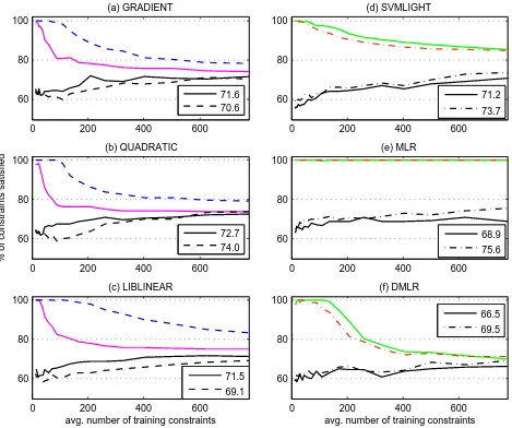
con-straints. Further tests on the unused training data repro-duce the results on the static test sets shown here. As shown in Figure 3, all algorithms are able to satisfy the initial training constraints. With the exception of MLR, (see Section 4.2), the training performance decreases for growing training sets, asymptotically approaching the test set performance. Such effects have been shown in [13] not to contradict good generalization results.

4.1 Impact of Model Complexity

For the facet-based linear approaches (Figure 3, left), a strong impact of the number of facet weight parameters can be observed. Whilst the performance for the model with 155 facets is significantly superior on the training data, it is generally worse on the test data. Only for a high number of training constraints, the simpler model with 26 facets can be matched or slightly outperformed. This is a strong indicator for model overfitting. With its many parameters, the complex model adapts too much to the training data at the cost of a reduced ability to generalize. In contrast, the simple model is able to generalize much quicker. This is especially remarkable for the quadratic programming ap-proach with the quickest generalization of all apap-proaches. Its adaptation performance on the test data also comes clos-est to the training performance, which can be seen as an upper bound. It appears as if this limit is increased by about 5%, if 155 facets are used instead, but more train-ing examples would be needed to get closer to this value. Here lies great potential for future research: By adapting the model complexity (i.e., the number of parameters) de-pending on the number of training examples and the per-formance on some unseen constraints, the ability of simple models to quickly generalize could be combined with the superior adaptability of more complex ones.

4.2 Effects of Similarity Sampling

For most of the algorithms tested, the effect of choosing sampling A or sampling B is small. Best performing are MLR (samling A) and quadratic programming(m= 155) for sampling B. Except for MLR, decrease in test set per-formance is limited to 1% when trained with the clip-sepa-rating sampling B. In the right column ofFigure 3, the met-ric learning algorithms are compared. The bottom black curves represent the test set results for sampling A (dashed,

· – ·) and sampling B (solid, —). The training perfor-mances for these samplings are plotted on the top of the graphs. While SVMlight(d) andDMLR(f) only loose 2-3% in performance, MLR (e) drops by more than 6%. Exclu-sively among the algorithms tested, the fully parametrized MLR(e) variant shows a 100% training performance for all training sizes. In line with results from Wolff et al. [13,14], the algorithm generalizes well on the similarity data with sampling A. Even with further permutations of the data, this capability to generalize reduces significantly when us-ing MLR with our samplus-ing method B, possibly caused by the lack of feature reoccurence in the training data.

5. CONCLUSIONS

The results of the experiment show that all approaches can adapt a similarity model to training data and generalize the learned information to unknown test data. Training perfor-mance curves can be used as an indicator for the maximal generalization outcome to expect, which depends on the number of facets and the features used. Sensitivity with re-spect to the sampling method of the test data was observed for MLR, which requires further investigation. Another promising direction for future work is to dynamically adapt the model complexity, e.g., by regularization. The feature data and sampling information are available online8 _for

benchmarking of approaches developed in the future.

6. REFERENCES

[1] K. Bade, J. Garbers, S. Stober, F. Wiering, and A. N¨urnberger. Supporting folk-song research by au-tomatic metric learning and ranking. InProc. of IS-MIR’09, 2009.

[2] K. Bade, A. N¨urnberger, and S. Stober. Everything in its right place? learning a user’s view of a music collec-tion. InProc. of NAG/DAGA’09, Int. Conf. on Acous-tics, 2009.

[3] W. Cheng and E. H¨ullermeier. Learning similarity functions from qualitative feedback. InProc. of EC-CBR’08, 2008.

[4] J. Donaldson and P. Lamere. Using visualizations for music discovery. Tutorial atISMIR’09, 2009.

[5] D. P. W. Ellis, B. Whitman, A. Berenzweig, and S. Lawrence. The quest for ground truth in musical artist similarity. InProc. of ISMIR’02, 2002.

[6] T. Joachims, T. Finley, and C.-N.J. Yu. Cutting-plane training of structural SVMs. In Machine Learning, 2009.

[7] E. Law and L. von Ahn. Input-agreement: a new mech-anism for collecting data using human computation games. InProc. of CHI ’09, 2009.

[8] B. McFee and G. Lanckriet. Heterogeneous embedding for subjective artist similarity. InProc. of ISMIR’09, 2009.

[9] B. McFee and G. Lanckriet. Metric learning to rank. In

Proc. of ICML’10, 2010.

[10] M. Schultz and T. Joachims. Learning a distance metric from relative comparisons. InNIPS, 2003.

[11] S. Stober. Adaptive distance measures for exploration and structuring of music collections. InProc. of AES 42nd Conference on Semantic Audio, 2011.

[12] S. Stober and A. N¨urnberger. An experimental com-parison of similarity adaptation approaches. InProc. of AMR’11, 2011.

[13] D. Wolff and T. Weyde. Adapting metrics for music similarity using comparative judgements. InProc. of ISMIR 2011, 2011.

[14] D. Wolff and T. Weyde. Adapting Similarity on the MagnaTagATune Database InACM Proc. of WWW’12, 2012.

0 100 200 300 400 500 600 700 60

65 70 75

avg. number of training constraints

% of test constraints satisfied

MLR 75.58% SVMLIGHT 73.72%

LIBLINEAR 72.21% GRADIENT 72.21% QUADRATIC 71.74% DMLR 69.53%

Figure 2. Performance comparison of facet-based approaches (with 26 facets) and metric learning. Values are averaged over all 20 folds of sampling A. The baseline at 63% refers to the mean performance of random facet weights (n= 1000).

0 200 400 600

60 80 100

avg. number of training constraints (c) LIBLINEAR

71.5

69.1

0 200 400 600

60 80 100

(a) GRADIENT

71.6 70.6

0 200 400 600

60 80 100

% of constraints satisfied

(b) QUADRATIC

72.7 74.0

0 200 400 600

60 80 100

(e) MLR

68.9

75.6

0 200 400 600

60 80 100

avg. number of training constraints (f) DMLR

66.5

69.5

0 200 400 600

60 80 100

(d) SVMLIGHT

71.2

73.7

Figure 3. Detailed performance of the individual approaches under different conditions. Top curves show training performance, bottom curves and legend show test set performance. Left column (a, b, c): Performance of the facet-based approaches using 26 facets (—) and 155 facets (– –). Comparison based on sampling B. Right column (d, e, f):