Interactive visual analysis of temporal cluster structures

City, University of London Institutional Repository

Citation:

Turkay, C., Parulek, J., Reuter, N. and Hauser, H. (2011). Interactive visual

analysis of temporal cluster structures. Computer Graphics Forum, 30(3), pp. 711-720. doi:

10.1111/j.1467-8659.2011.01920.x

This is the unspecified version of the paper.

This version of the publication may differ from the final published

version.

Permanent repository link:

http://openaccess.city.ac.uk/3617/

Link to published version:

http://dx.doi.org/10.1111/j.1467-8659.2011.01920.x

Copyright and reuse: City Research Online aims to make research

outputs of City, University of London available to a wider audience.

Copyright and Moral Rights remain with the author(s) and/or copyright

holders. URLs from City Research Online may be freely distributed and

linked to.

Eurographics / IEEE Symposium on Visualization 2011 (EuroVis 2011) H. Hauser, H. Pfister, and J. J. van Wijk

(Guest Editors)

Volume 30 (2011), Number 3

Interactive Visual Analysis of Temporal Cluster Structures

C. Turkay1, J. Parulek1, N. Reuter2, and H. Hauser1

1_{Department of Informatics, University of Bergen}2_{BCCS, University of Bergen}

Abstract

Cluster analysis is a useful method which reveals underlying structures and relations of items after grouping them into clusters. In the case of temporal data, clusters are defined over time intervals where they usually exhibit structural changes. Conventional cluster analysis does not provide sufficient methods to analyze these structural changes, which are, however, crucial in the interpretation and evaluation of temporal clusters. In this paper, we present two novel and interactive visualization techniques that enable users to explore and interpret the structural changes of temporal clusters. We introduce the temporal cluster view, which visualizes the structural quality of a number of temporal clusters, and temporal signatures, which represents the structure of clusters over time. We discuss how these views are utilized to understand the temporal evolution of clusters. We evaluate the proposed techniques in the cluster analysis of mixed lipid bilayers.

Categories and Subject Descriptors (according to ACM CCS): Computing Methodologies [I.3.m]: Computer Graphics—Miscellaneous

1. Introduction

With the advance of data acquisition and simulation systems, large amounts of data with a high number of dimensions and temporally varying values are produced. In various fields like bioinformatics, financial analysis and engineering, it is of great importance to explore and understand the groups of data which share common characteristics over time. These groups are usually analyzed further to gain insight into the processes that are governed by these common characteris-tics. Cluster analysis is a widely used method to discover grouping structures in both static and time-varying data. This analysis results in a set of clusters, each of which represents a group of similar items with respect to certain features of the data. However, when performing cluster analysis on tempo-ral datasets, interpreting and evaluating the resulting clusters is not as straightforward as it is with static data.

Most of the algorithms developed for clustering time se-ries (temporal) data are either modifications of the static data clustering algorithms, or time-series are converted into static representations such that existing algorithms can be used [Lia05]. Therefore, these clustering algorithms focus mainly on the design of a proper distance function to use in clustering or in the conversion of the data into fea-ture vectors of lower dimensionality. These custom distance functions and conversion operations applied to large,

high-dimensional time series may easily produce low-quality clusters [WSH06]. As a consequence, the interpretation and evaluation of clusters become a very important part of clus-ter analysis. Current methods for clusclus-ter assessment, how-ever, are mainly tailored for static data [Lia05], yielding a need for new mechanisms to analyze temporal clusters.

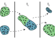
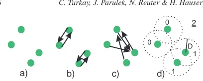
In the following, we illustrate a simple situation where advanced analysis techniques are required to understand the variation of time-dependent cluster structures. We consider a simple scenario as illustrated in Fig.1. In this setting, two well separated and equally sized groups merge into a sin-gle, heterogeneous group at time t1and split into two groups again at time t2. This simple scenario demonstrates a typi-cal example of structural changes which clusters can exhibit over time. Also note that, clustering different time intervals (i.e., t0, t1or t2) yields completely different clusters.

conse-t0 t1 t2

Figure 1: An example of structural changes in clusters of

temporal data. Two well-separated clusters (at t0) merge into a single group at t1and split into two groups again at t2.

quently discard or update the clusters. The analysis of these variations are not really addressed by the current methods and techniques in cluster analysis. In order to interpret and evaluate temporal clusters, the analyst has to answer at least two questions; firstly, "How does the quality of clusters vary over time?" and secondly, "What type of structural changes do clusters exhibit?".

In this paper, we propose two novel and interactive visu-alization techniques to analyze temporal clusters. We firstly introduce the temporal cluster view that visualizes the struc-tural quality of temporal cluster sets over time. Secondly, we present temporal signatures which are visual summaries of temporal cluster structures. The cluster view provides mech-anisms to visualize and interactively analyze a set of tem-poral clusters that are computed from different time inter-vals. This view also encodes silhouette coefficients [Rou87], which are quite widely used cluster structure metrics. They are used to evaluate the structural quality of cluster sets. Temporal signatures are representations of statistical prop-erties of clusters over time. These propprop-erties are based on cluster cohesion which represents the tightness of its items, and cluster homogeneity which correspond to the uniformity of the distribution of the member items [TSK06].

When used in conjunction, these two views provide in-tuitive mechanisms to analyze and evaluate temporal ters. They are utilized to explore structural changes in clus-ters; namely, splitting, merging, and changes in cluster size. We present these two views in an interactive visual analysis framework. To summarize, our contributions in this paper are:

• The temporal cluster view, visualizing a number of tempo-ral clusters together with their structutempo-ral quality variation.

• Temporal signatures, that are visual representations of the structural changes of groups over time.

• Interactive visual analysis procedures for temporal cluster analysis with the help of these two views.

2. Related Work

Our work relates to the analysis of temporal clusters using interactive techniques and visual representations for

tempo-rally varying structures. Thus, the related literature is pre-sented in three subsections:

Analyzing clusters – Vectorized radial visualizations are used in exploring different clustering results by projecting data records on a vectorized cluster space [SGM08]. This approach proves to be useful in validating the clusters when a number of cluster sets for the same dataset exist. Rinzivillo et al. proposes a visually guided clustering called progres-sive clustering [RPN∗08], where the clustering is done with different distance functions in successive steps. In hierarchi-cal clustering explorer [SS02], Seo and Shneiderman use an interactive dendogram, coupled with a color mosaic to rep-resent clustering information in a linked visualization. They propose a cluster comparison view where two clustering re-sults can be compared. However, their method is only suited for clusters of static data. In a recent study, Lex et al. in-troduce the MatchMaker [LSP∗10], visualizing and com-paring multiple groups of dimensions to represent cluster memberships. Their cluster visualization method is similar to our temporal cluster view, however, their solution does not provide information on the structural quality of clus-ters over time. Moreover, their method is designed for static clusters only. In the MultiClusterTree [VLL09], Long and Linsen discuss how clusterings are utilized to analyze multi-dimensional data. They use a radial layout, linked with sev-eral other views to explore hierarchical clusters. Telea and Auber [TA08] visualize changes in code structures using a flow layout where they try to identify steady code blocks and when certain splits in the code occur.

C. Turkay, J. Parulek, N. Reuter & H. Hauser / Interactive Visual Analysis of Temporal Cluster Structures 3

Visual representations of temporal data – In this paper, we provide visual a representation of the structural changes of temporal clusters. There is a large number of studies on how to represent temporal data in visualization [WAM01, Moe05]. One of the important studies which represents tem-poral changes visually is the ThemeRiver [HHWN02] by Havre et al. The authors provide a visual representation of thematic changes in document collections over time. The ThemeRiver visualizes a single value per item and proposes a cumulative representation for each time step. In our tempo-ral signatures, however, we encode a number of tempotempo-rally varying statistics that are not suitable for a cumulative visu-alization due to their different scales.

In this paper, we extend the state of the art in the visual analysis of temporal clusters with the temporal cluster view, that integrates temporal clusters into interactive visual anal-ysis procedures, and temporal signatures that visualize the temporal structure of clusters.

3. Overview

The proposed solution for analyzing temporal clusters is based on a new temporal cluster view (in the following just "cluster view") and temporal signatures. Firstly, we intro-duce the cluster view, that visualizes the quality of clus-ters together with structural changes that are related to item-cluster and cluster-cluster relationships. Secondly, we present temporal signatures, which are visual summaries of the statistical properties of clusters over time. The variations of these statistical properties reveals structural changes in groups of items.

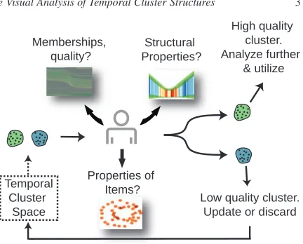
These two views are utilized in an interactive visual anal-ysis (IVA) cycle to analyze temporal clusters. Prior to the analysis, the analyst constructs a set of temporal clusters using a clustering algorithm. Information from the cluster view and the temporal signatures are combined with infor-mation on properties of items as provided by conventional views. The resulting insight is used to interpret and/or vali-date the clusters. This analysis is performed iteratively until sufficient clusters and insight in group relations is achieved. Fig.2is an overview illustration of our solution.

We present our solution in an IVA framework where we incorporate different types of linked views: histograms, scat-terplots, parallel coordinates, (for regular variables), and functions graphs and animated scatterplots for temporal vari-ables. In order to update these temporally varying views syn-chronously, we use a global time parameterτ. We define the dataset of independent variables (items) as O={o1, . . . ,on}, where each item has a set of m= p+q dependent val-ues F(oi) = [f1(oi), . . . ,fp(oi),gp+1(oi,t), . . .,gp+q(oi,t)]. Here, f represents regular variables and g represents time-series which are defined over time interval[0,t′]. We define a temporal cluster cias:

ci={Ici,Tci: Ici⊆O,Tci= [t0,t1],0≤t0≤t1≤t′} (1)

Memberships, quality?

Structural Properties?

Properties of Items?

Low quality cluster. Update or discard

High quality cluster. Analyze further

& utilize

Temporal Cluster

Space

Figure 2: An overview of our approach. A subset of

tem-poral clusters are analyzed using our techniques and con-ventional IVA tools in terms of their structural changes and quality variations. Plausible clusters are analyzed to derive more insight on data. Low quality clusters are updated or discarded.

In order to obtain such clusters, the analyst first defines a time interval T and then uses a clustering algorithm to cluster the data in T . This clustering operation is performed k times using different time intervals and/or item subsets which are determined by the user. We refer to the set of clusters ob-tained at each such step as a clustering Cjand the set of all the clusterings as U={C0, ..,Ck}where Cjis defined as:

Cj={c1, ..,cnj:∀ca,cb(Tca=Tcb∧ca6=cb⇒ca∩cb=∅)} (2) with nj as the total number of clusters in Cj. Additionally, we do not necessarily expect Cj to include all the items in O, i.e.,Sc∈Cj⊆O. Note that in a clustering, there are no overlapping clusters in terms of their items. However, it is possible that temporal spans of clusterings can overlap. In this paper, we use both hierarchical and k-means cluster-ing [TSK06]. As these algorithms are originally developed for static data, we modified the distance measures as sug-gested by Liao [Lia05]. Our solution is well-suited to tem-poral versions of hierarchical and partitioning clustering al-gorithms, as they operate on distances between items. How-ever, there exist also other algorithms which operate on den-sities and statistical models [Lia05]. To generalize our ap-proach to a wider-variety of algorithm results, different qual-ity metrics needs to be included into the analysis procedure.

1

₂

3

4

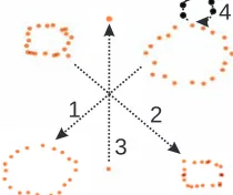
Figure 3: In this artificial dataset, two groups move towards

each other following the paths 1 and 2. One point follows path 3 and one item shortly gets away from its group (4).

∩represents the intersection and¬represents the not oper-ator. The result of this combination is a composite brush B, which is computed "in parallel" as the user makes brushes. Individual brushes biare combined into composite brushes Bi using the selected S by Bi= S(Bi−1,bi) starting with B1=S(b0,b1). For simplicity, in the following, we denote the final set of brushed items as BL={IL,TL}. Note that, our definitions of a brush and a cluster (1) is the same, i.e., b=

{I,T}=c. This enables the interpretation of clusters directly as brushes in our system. Due to the fact that non-continuous selections with respect to time would cause an additional complexity in the temporal analysis and related calculations,

∪operator on time results in a single continuous time in-terval. The resulting time interval encapsulates both input intervals, i.e.,[t0,t1]∪[t2,t3] = [min(t0,t2),max(t1,t3)]. One other exception in the brushing mechanism is related to the

∩operator in the temporal cluster view. In this view, when two brushes are combined using∩, the item groups are in-tersected as expected with∩. The temporal spans, however, are joined using∪. This modification enables the use of the

∩operator between clusters defined over non-overlapping temporal spans.

In order to demonstrate our approach in the following, we consider an artificial dataset (Fig.3). In this dataset, two groups, composed of 20 points each, merge and split at cer-tain points in time. There is a point that moves vertically from the bottom to the top. Additionally, one point shortly gets away from its group and returns back at the first half of the sequence. Prior to the analysis of this dataset, a number of clusterings are added to U . In order to avoid extra com-plexity in the analysis, we use all the items in consecutive clustering operations.

4. The Temporal Cluster View

The proposed temporal cluster view enables the visual ex-ploration of clusters which are defined over different time intervals. It visually depicts how cluster memberships evolve over time. Moreover, it encodes cluster quality metrics and enables cluster level selections.

In the cluster view, each vertical axis visualizes a cluster-ing Ck, where k indicates the order of the clustering in the view, i.e., for the leftmost axis, k=1 (Fig.4a). Each rectan-gle on an axis corresponds to cluster cki in Ckand each curve between the axes represents a single data item, oi. When the user selects a cluster c in this view, Icand Tcare handled by the selection mechanism as any other brush b with the above mentioned exception related to the∩operator.

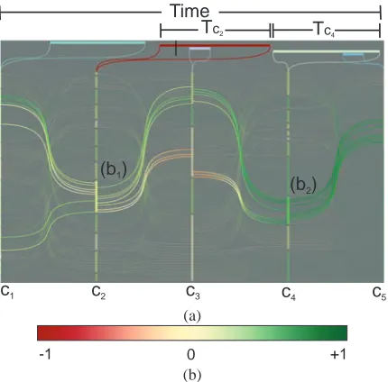
We visualize the temporal span of clusters in order to link this view to the other temporally updating views. In Fig.4a, five clusterings C1−5, performed on different time intervals, are visualized together with their temporal span on top. A black cursor is displayed at the top of the view to indicateτ. Temporal span of the clusterings, which are defined atτ, are highlighted by a saturated red color at the top of the view, e.g., C2in Fig.4a. Here, brushes b1and b2 are combined using the∩operator, selecting the intersection of the items and the union of the temporal spans.

In order to encode information about the structural qual-ity of clusters, we utilize the silhouette coefficient [Rou87], which is a popular method in data mining for evaluating the structural quality of clusters. Silhouette values ski are com-puted per each item of cluster ck_i and they are in the range [−1,1]. Items close to cluster centers have higher values, and items on the borders of a cluster with close neighboring clus-ters have values close to 0. Moreover, when an item has a sil-houette value close to−1, this item is wrongly placed in this cluster as an artifact of the clustering algorithm. In cluster view, we use silhouette values to color code curves and clus-ter rectangles. The color coding map, extracted from Color-Brewer [Bre09], is included in Fig.4b. The color of a single curve is interpolated between ski and ski+1and each cluster rectangle is colored according to the average of the skivalues of its members. Here, green colored curves and/or rectan-gles represent high-quality clusters (with respect to silhou-ette values).

In the cluster view, ordering is crucial for the ease of in-terpretation. Firstly, we order clusterings Ckaccording to the "start" of their time intervals TCk. Secondly, the c

k i on each axis are ordered with a greedy algorithm in order to min-imize overlapping curves between clusters. This ordering starts with the first clustering C1placed randomly. The al-gorithm then continues with the bottom-most cluster c1₁of C1and finds the cluster x∈C2which has the biggest overlap with c1₁, i.e., arg max_x∈C2

c

1 1∩x

. Then x is placed to the first

out-C. Turkay, J. Parulek, N. Reuter & H. Hauser / Interactive Visual Analysis of Temporal Cluster Structures 5

c

c

c

c

c

Time

T

(b )

(b )

T

(a)

-1 0 +1

(b)

Figure 4: (a) Five clusterings visualized in the cluster view.

The temporal span of each clustering is visualized on top. Brushes b1and b2are made to select two clusters. (b) Color coding for silhouette values.

come for the requirements of our solution. Finally, we or-der the items in the clusters. All the members of the clusters are first grouped according to the branches between Ckand Ck+1, where a branch represents overlapping items between two clusters, i.e., ck_i∩ck_j+1. As the final step in this ordering, all the items in a single branch are organized in an ascend-ing order with respect to sk_i values. The effect of ordering on the perception of cluster relations and cluster quality is illustrated in Fig5.

Although our clustering definition (2) allows for items that are not members of any clusters, the clustering algo-rithms we use in this paper assigns all the items to clusters. In case of items which are not in a cluster (can be referred to as outliers), these items are grouped together and visualized just like any other cluster in the cluster view. If the analyst plans to focus on these outliers, this group of outlier items can be visualized in a distinctive color in the cluster view.

5. Temporal Signatures

In order to explore the structural changes in temporal clus-ters, we rely on a qualitative approach based on structural statistics, which is easy to interpret, calculate, and visual-ize. Fig.6demonstrates the proposed measures. We utilize a group coherence measure that is based on mutual distances between items in ILfor every time step in TL. Note that ILcan consist of any group of items that are selected by the brush combinations in the framework. Here, we compute average

a)

b)

Figure 5: Ordering cluster view improves the overall

per-ception of cluster quality. Before (a) and after ordering (b).

distance boundaries, which can be thought of as comput-ing the extent covered by points IL—referred to as cluster diameter [ELL09]. The minimum average distance Mintavg and maximum average distance Maxtavg are calculated for all time steps separately as follows:

Mintavg= ∑

|IL| i=1d

t min(oi) |IL|

, (3)

where d_mint (oi) =min({dt(oi,oj)|oi,j∈IL∧oj6=oi})and t represents a single time step. Maxtavg is computed like-wise with max instead of min in equation (3). Per each time step, we additionally compute the sum of number of items "closer" to each other than a distance threshold D. This num-ber, which we refer to as vicinity measure V , describes the compactness (cohesion) of the group [TSK06]. D is a free parameter, which users can interactively change according to the Minavgand Maxavgvalues. Vt(D)is defined by:

Vt(D) =

|IL|

∑

i=1

{j|oj∈IL∧oj6=oi∧dt(oi,oj)<D}

. (4)

For equations (3) and (4), the Euclidean distance is preferred for dt(·,·), which is defined as: dt(oi,oj) =

q ∑q

k=1 gk(oi,t)−gk(oj,t)2

a) b) c) d)

D

1

2

1 0

0

Figure 6: For four 2D points (a), we compute minimum

dis-tances (b), maximum disdis-tances (c), and vicinity measure V (d). V is the sum of neighboring items within a sphere of radius D (0+0+1+1=2).

The temporal signature view computes the above defined metrics for the currently selected group of items (not nec-essarily from a cluster) over the selected time interval to construct the visualization. Fig.7(left) shows an example of such a temporal signatures view, where IL contains all the items for the whole time span of the dataset. The up-per bound represent maximum average distances, while the lower one represent minimum average distances. We also compute the standard deviations of these distances and ren-der them in a transparent green band around the actual min-imum and maximal values. Moreover, we utilize the space between the boundaries to display V values by color intensi-ties. The saturated blue colors represent sparsely distributed items, while the saturated red colors represent packed items, i.e., higher number of neighboring items. The color scaling is done according to the minimum and the maximum values of V for the current ILand TL. In Fig.7(left), we can observe an instability between Minavgand Maxavgvalues, where the band gets thinner in the middle as time progresses. This is due to the fact that the groups at t0 cross each other at t1 making the overall cluster diameter smaller.

Both standard deviations, stdev(Minavg) and stdev(Maxavg), encodes cluster homogeneity. In Fig.7, we select first IL=c1, then IL=c2, and eventually IL=c1∪c2 over TL= [t0,t1]. The signature of cluster c1 indicates a high quality cluster due to the stable values of the metrics. However, cluster c2 contains an outlier (Fig. 3-4), that is recognized through the peaking standard deviations. In general, stdev(Minavg) reveals outliers. stdev(Maxavg) is mainly associated with cluster homogeneity where lower values identify tightly packed items or groups of such tightly packed items. For instance, although group c1∪c2, separates at t0, the resulting stdev(Maxavg) values do not vary when c1and c2merges at t1, except for the outlier in c2.

For all the views in Fig.7, we specify D=max{Minavg}, which means that there is a number of items above D for all the time steps. This choice of D reveals only the most com-pact configuration of the items over the whole time interval. In the rightmost signature view in Fig.7, it can be seen that items are in the most compact form at t2(saturated red color) where c1and c2merges.

Instead of arbitrary groups of items, the analyst can prefer to directly brush clusters. In this case, the signature view enables the user to perform a number of analysis tasks on clusters:

• A single cluster can be visualized to evaluate its temporal structural variations.

• A number of clusters can be brushed using S operators to explore the resulting group’s behaviors.

• While a single cluster is selected, the temporal selection (TL) can be expanded using other brushes. The resulting signature view visualizes how this cluster behaves over time intervals where it is not defined.

6. Temporal Cluster Analysis Procedures

Temporal-cluster analysis aims to find a plausible set of clus-ters and understand the structural variations of these clusclus-ters. The analysis starts with visualizing the selected clusterings in the cluster view and continues with selecting a number of clusters and investigating the corresponding temporal signa-tures. As a result of the interpretations of these two views, the analyst draws one of these conclusions; validate a clus-ter, update the temporal span of a cluster or discard a cluster. In order to draw such conclusions, interpretation of silhou-ette values and discovering where structural changes (like splitting and merging) take place is quite important.

Interpreting silhouette values – Silhouette values are higher when the clusters are well-separated and more coher-ent. Therefore, in regions with not so apparent clusters (i.e., where the distribution of items is more uniform), the silhou-ette values are generally close to zero or even below zero. In

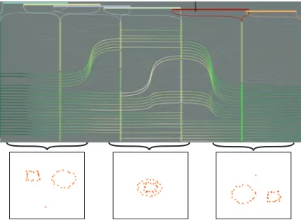
Fig.8, we can see a clear example of such a situation. Here,

the example dataset (Fig.3) is clustered over consecutive time intervals (C1−6). As the distribution of items where two groups meet is quite uniform, we see that the colors of items and clusters turn to yellow. However, near the beginning and at the end of the sequences, the overall cluster quality is high, and this is clearly visible from the colors of C1and C6. This observation yields to the fact that clusters performed over the merging interval are lower in structural quality and therefore, have to considered with more care when further analysis is performed on them.

Merging and splitting – Two of the important behavior of clusters are merging and splitting. To analyze these behav-iors, we firstly brush a cluster by∩operation, which may represent a cluster that is about to split or to be created as a union of several other clusters. Secondly, we observe the accompanied temporal signatures view, which reveals this structural tendencies.

C. Turkay, J. Parulek, N. Reuter & H. Hauser / Interactive Visual Analysis of Temporal Cluster Structures 7

t0

[t0,t1]} t1

t2 Max

stdev(Max)

D

Min

Time

Distance

stdev(Min)

avg

avg

t0 t1 t2 min(V) max(V)

[t0,t1]}

[t0,t1]} c1 c2

{c ,1

{c ,2

{c U₁ c2,

Figure 7: Left: Temporal signatures view. The upper bound represents maximum average distance, the lower represents

min-imum average distance and the vicinity measure is represented with the color map depicted on the bottom right. The dotted line represents the threshold distance D. The standard deviation is rendered through the transparent green color. Circles mark changes due to movement 4 in Fig.3. Right: Signature views computed for clusters c1, c2and c1∪c2over time interval[t0,t1].

Figure 8: Variation of silhouette values. Group structures

change as items move over time. These variations are clearly visible in cluster view by observing the color changes.

and C2. The signatures view is then automatically updated for IL=IC2 and[TC1∪TC3]. A notable tendency is that the band between the Minavg and Maxavg gets smaller towards TC2 (cluster merging) and gets large again at TC3 (cluster splitting). We can additionally observe that ILhas the most compact form where both groups merge and a sparse form where the groups are separated by observing V values.

To generalize, we follow a set of informal rules in evalu-ating the clusters using our views:

• Items in a cluster should not have many branchings in cluster view

• Cluster rectangle and item curves should be in saturated green

• In a signature of a cluster, values of Minavgand Maxavg

and the thickness of the band between them should not deviate

• Signatures should mostly contain red values in the band (i.e., high V values)

7. Case Study: Analysis of Molecular Dynamics of Mixed Lipid Bilayers

Molecular modeling of biological membranes is one of the application fields where analysis of temporal clusters is par-ticularly useful. Cell membranes separate the interior of cells from the environment and are mostly constituted of a mix-ture of different lipids. The lipids can form microdomains or clusters with other membrane components. Such mi-crodomains are relevant for signal transduction or cell apop-tosis to name but a few [FSH10]. Lipid bilayers are widely used to model and study cell membranes, and molecular dy-namics (MD) simulations are utilized as powerful tools to describe their atomic structure and dynamic behavior. These simulations run on a mixture of different types of lipids that form different cluster sets. These lipid clusters can lead to inhomogeneity in biological membranes [BR10].

Here we use a dataset obtained from MD sim-ulation of a mixed lipid bilayer [BR10], constituted of DMPC (dimirystoilphosphatidylcholine) and DMPG (dimirystoilphosphatidylglycerol) lipids composed of 1640 time steps. Each lipid is represented by one particle, local-ized at the position of the phosphorus atom. Additionally, we work on a set of clusterings{C1, . . . ,Cn}that are computed as the final step of the simulation phase.

t=t2

t2 t4

t=t0

t0

t=t1

t=t4

t1

(b ) (b )

(b ) 1

2

3

a) b)

X X

X

X X

X

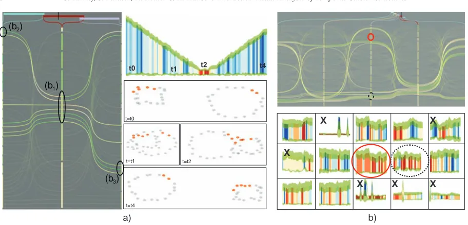
Figure 9: a) Cluster merging-splitting behavior. A cluster is selected with b1and the time selection is enlarged by brushes b2 and b3. Merging occurs around the smaller band in the middle, which gets larger at end of the sequence due to splitting in signature view. b) Searching for a plausible cluster. Two good signatures are identified (circles). The dashed circle is discarded due to its structural instability in cluster view (shown with the selection on the right). The red circled cluster is picked for further analysis. Moreover, the observed signatures allow to discard clusters (X) according their structure.

We start the analysis by displaying the clusterings in the cluster view. Then we assess the cluster quality, firstly, by brushing individual clusters by∩operation according to sil-houette values, and secondly, assessing the cluster coherence via the signature view. Here, we use the set of rules described in Section6. Fig.9b displays a set of signatures for the ob-served clusters C1−5 defined over sequential time intervals TC1−5.

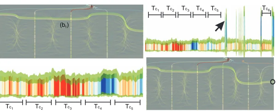
In Fig.9b, although the signature for the cluster marked with dotted circle represents a good cluster; the cluster struc-ture over time is not stable due to branching in cluster view. Therefore, this cluster is not picked for further analysis. Dis-carded clusters are marked with an X in the figure. Neverthe-less, we found a cluster (marked with a red circle in Fig.9b) that has a plausible signature and exhibits a stable struc-ture in the neighboring clusterings. We continue our analysis with this cluster c in C3(Fig.10). As the next step, we en-large the time selection, from TL=TC3to TL= [TC1∪TC5]. The corresponding signature Fig. 10 (left-bottom) depicts the stability of cluster c even for the remaining intervals. The stability is observed by the band width between min-imum average distance Minavgand maximum average dis-tance Maxavg. The group extend is preserved over TLsince stdev(Maxavg)has the same width for the whole time. How-ever, stdev(Minavg)exhibits certain instabilities which are caused by oscillation movements of cluster boundary lipids that gets away from the group for a few time steps. Addi-tionally, we continue by extending time interval TLwith a

brush on time domain (not shown in the figure) to analyze how stable this group is over a larger time interval. With this update, we observe that the signature changes rapidly for lat-ter regions (Fig.10(top-right)). This limits the time extend of this cluster to the first peak (arrow). However, later on, we can see that the vicinity values, depicted by colors, are close to red again, identifying that the same group is form-ing. Since we observe this region where the cluster can be defined, we add clustering C6for this region of interest. We see in Fig.10(bottom-right) that cluster c is formed again, even for this small interval.

bilay-C. Turkay, J. Parulek, N. Reuter & H. Hauser / Interactive Visual Analysis of Temporal Cluster Structures 9

Tc₅

Tc6

Tc1

Tc1

Tc2

Tc2

Tc3

Tc3

Tc4

Tc4 Tc5

(b )1

Figure 10: Lipid cluster development. Top left: Coherent cluster c=b1in all clusterings, C1−5. Bottom left: The signature view for c with extended time interval to showcase signatures in remaining clustering intervals TL= [TC1∪TC5], where it expresses high stability. Top right: We extend TLto search for "existing" boundaries (arrow) for cluster c, where we mark another coherent interval TC6. We add cluster C6, where we observe that items in b1reforms cluster c again at TC6(circle).

ers. During this case study, we came across a number of additional analysis tasks like: identifying the threshold de-viations for the "good" lipid clusters, analysis of vanishing clusters and determining the time when the overall system stabilization takes place. These are potential tasks where our analysis framework can be utilized. In general, our collab-orators find the procedure to be faster, more powerful and more reliable than traditional approaches which are usually based on distance criteria applied to each frame of the se-quence.

8. Conclusion

In this paper, we introduce two novel visualization tech-niques for the interactive visual analysis of temporal clus-ters. We firstly introduce cluster view, which interactively vi-sualizes a number of clusters defined on temporal intervals. This view visualizes the variation of the structural quality of clusters by representing the changes of silhouette coeffi-cients. Cluster view visualizes the temporal span of clusters in order to enable the exploration of clusters over time. Sec-ondly, we present temporal signatures which are visual rep-resentations of the structure of a group of items over time. This view encodes a number of time-varying statistical prop-erties of a group to depict its structural transformations. We show how these views enable an intuitive analysis of tem-poral clusters, where the analyst is able to determine the va-lidity of the clusters and interpret the relations that cause structural changes in clusters. To the best of our knowledge, our solution is the first interactive visual approach to analyze the structural changes in cluster-cluster and item-cluster re-lations of temporal datasets.

We integrated our visualizations into an IVA environment where we performed visual analysis of temporal clusters. Cluster view enables cluster level interactions and when used in combination with temporal signatures view, it pro-vides a mechanism to explore temporal clusters in terms of their structural properties. We describe analysis procedures which enables the analyst to explore the quality of clusters over time and explore the structural changes exhibited by clusters. As a consequence of these analyses, the clusters are either validated, updated or discarded. The analyst then con-tinues with the further analyses of high quality clusters.

We evaluated our methodologies on the analysis of molec-ular dynamics simulation, where the analyst is trying to build hypotheses on the grouping behaviors of lipid-bilayers. We show that our methods reveals certain groups which exhibit stable behavior over distinct time intervals. Such behavior patterns provides the basis to make hypotheses on the be-havioral properties of lipid bilayers.

As a future work, we plan to extend our temporal signatures with more robust statistics and different quality metrics, which can provide deeper insight on the structure of groups of items. Another future direction is to create abstract representations of the structural changes and encode them in the form of an event based visualization system.

Acknowledgments

References

[AAB∗_{10] ANDRIENKO G., ANDRIENKO N., BREMM S.,}

SCHRECKT., VON LANDESBERGERT., BAK P., KEIMD.: Space-in-time and time-in-space self-organizing maps for explor-ing spatiotemporal patterns. Computer Graphics Forum 29, 3 (2010), 913–922.2

[AAR∗_{09] ANDRIENKOG., ANDRIENKON., RINZIVILLOS.,}

NANNIM., PEDRESCHID., GIANNOTTIF.: Interactive visual clustering of large collections of trajectories. In Visual Analytics

Science and Technology, 2009. VAST 2009. IEEE Symposium on

(2009), IEEE, pp. 3–10.2

[BR10] BROEMSTRUPT., REUTER N.: Molecular Dynamics Simulations of Mixed Acidic/Zwitterionic Phospholipid Bilay-ers. Biophysical journal 99, 3 (Aug. 2010), 825–833.7,8

[Bre09] BREWERC. A.: http://www.colorbrewer.org/, 2009.4

[ELL09] EVERITTB. S., LANDAUS., LEESEM.: Cluster

Anal-ysis, 4th ed. Wiley Publishing, 2009.5

[FSH10] FANJ., SAMMALKORPIM., HAATAJAM.: Formation and regulation of lipid microdomains in cell membranes: Theory, modeling, and speculation. FEBS letters 584, 9 (2010), 1678– 1684.7

[GRVE07] GROTTELS., REINAG., VRABECJ., ERTLT.: Vi-sual verification and analysis of cluster detection for molecular dynamics. IEEE Transactions on Visualization and Computer

Graphics 13, 6 (2007), 1624–1631.2

[HHWN02] HAVRES., HETZLERE., WHITNEYP., NOWELL

L.: Themeriver: Visualizing thematic changes in large document collections. IEEE Transactions on Visualization and Computer

Graphics 8 (January 2002), 9–20.3

[KW01] KAUFMANNM., WAGNERD.: Drawing graphs:

meth-ods and models. Springer Verlag, 2001.4

[Lia05] LIAOW.: Clustering of time series data–a survey. Pattern

Recognition 38, 11 (2005), 1857–1874.1,3

[LSP∗_{10] LEX A., STREIT M., PARTL C., KASHOFER K.,}

SCHMALSTIEGD.: Comparative analysis of multidimensional, quantitative data. Visualization and Computer Graphics, IEEE

Transactions on 16, 6 (2010), 1027 –1035.2

[Moe05] MOEREA.: Time-varying data visualization using in-formation flocking boids. In Inin-formation Visualization, 2004.

INFOVIS 2004. IEEE Symposium on (2005), IEEE, pp. 97–104.

3

[MW95] MARTINA. R., WARDM. O.: High dimensional brush-ing for interactive exploration of multivariate data. In VIS ’95:

Proceedings of the 6th conference on Visualization ’95

(Wash-ington, DC, USA, 1995), IEEE Computer Society, p. 271.3

[Rou87] ROUSSEEUWP.: Silhouettes: a graphical aid to the in-terpretation and validation of cluster analysis. Journal of

compu-tational and applied mathematics 20 (1987), 53–65.2,4

[RPN∗_{08] RINZIVILLOS., PEDRESCHID., NANNIM., GIAN} -NOTTIF., ANDRIENKON., ANDRIENKOG.: Visually driven analysis of movement data by progressive clustering.

Informa-tion VisualizaInforma-tion 7, 3 (2008), 225–239.2

[RWH∗_{10] RUBELO., WEBERG., HUANGM.-Y., BETHELE.,}

BIGGINM., FOWLKESC., LUENGOHENDRIKSC., KERANEN

S., EISENM., KNOWLESD., MALIKJ., HAGENH., HAMANN

B.: Integrating data clustering and visualization for the analysis of 3d gene expression data. Computational Biology and

Bioin-formatics, IEEE/ACM Transactions on 7, 1 (2010), 64 –79.2

[SGM08] SHARKO J., GRINSTEING., MARXK.: Vectorized radviz and its application to multiple cluster datasets. IEEE

trans-actions on Visualization and Computer Graphics (2008), 1444–

1427.2

[SS02] SEOJ., SHNEIDERMANB.: Interactively exploring hier-archical clustering results. IEEE Computer 35, 7 (2002), 80–86.

2

[SS05] SEBORGA., SINGHALA.: Clustering multivariate time-series data. Journal of chemometrics 19, 8 (2005), 427.1

[STH∗_{09] SHIK., THEISELH., HAUSERH., WEINKAUF T.,}

MATKOVICK., HEGEH., SEIDELH.: Path line attributes-an information visualization approach to analyzing the dynamic be-havior of 3d time-dependent flow fields. Topology-Based

Meth-ods in Visualization II (2009), 75–88.5

[TA08] TELEAA., AUBER D.: Code flows: Visualizing struc-tural evolution of source code. Computer Graphics Forum 27, 3 (2008), 831–838.2

[TSK06] TANP., STEINBACHM., KUMARV.: Introduction to

data mining. Pearson Addison Wesley Boston, 2006.2,3,5

[VLL09] VANLONGT., LINSENL.: MultiClusterTree: Interac-tive Visual Exploration of Hierarchical Clusters in Multidimen-sional Multivariate Data. In Computer Graphics Forum (2009), vol. 28, John Wiley & Sons, pp. 823–830.2

[VWVS99] VANWIJKJ., VANSELOWE.: Cluster and calendar based visualization of time series data. In infovis (1999), Pub-lished by the IEEE Computer Society, p. 4.2

[WAM01] WEBERM., ALEXAM., MÜLLERW.: Visualizing time-series on spirals. In proceedings of the IEEE Symposium on

Information Visualization (2001), Citeseer, p. 7.3

[WSH06] WANGX., SMITHK., HYNDMANR.: Characteristic-based clustering for time series data. Data Mining and