Vakhnenko, V.O. and Parkes, E.J. (2012) Special singularity function for
continuous part of the spectral data in the associated eigenvalue
problem for nonlinear equations. Journal of Mathematical Physics, 53
(6). ISSN 0022-2488 , http://dx.doi.org/10.1063/1.4726168
This version is available at
https://strathprints.strath.ac.uk/40092/
Strathprints is designed to allow users to access the research output of the University of Strathclyde. Unless otherwise explicitly stated on the manuscript, Copyright © and Moral Rights for the papers on this site are retained by the individual authors and/or other copyright owners. Please check the manuscript for details of any other licences that may have been applied. You may not engage in further distribution of the material for any profitmaking activities or any commercial gain. You may freely distribute both the url (https://strathprints.strath.ac.uk/) and the content of this paper for research or private study, educational, or not-for-profit purposes without prior permission or charge.
Any correspondence concerning this service should be sent to the Strathprints administrator:
The Strathprints institutional repository (https://strathprints.strath.ac.uk) is a digital archive of University of Strathclyde research outputs. It has been developed to disseminate open access research outputs, expose data about those outputs, and enable the
Special singularity function for continuous part of the spectral data in the
associated eigenvalue problem for nonlinear equations
V. O. Vakhnenko and E. J. Parkes
Citation: J. Math. Phys. 53, 063504 (2012); doi: 10.1063/1.4726168 View online: http://dx.doi.org/10.1063/1.4726168
View Table of Contents: http://jmp.aip.org/resource/1/JMAPAQ/v53/i6
Published by the American Institute of Physics.
Related Articles
Soliton-like solutions to the ordinary Schrödinger equation within standard quantum mechanics
J. Math. Phys. 53, 052102 (2012)
Integrability of nonlinear wave equations and solvability of their initial value problem
J. Math. Phys. 53, 043701 (2012)
Spontaneous soliton generation in the higher order Korteweg–de Vries equations on the half-line
Chaos 22, 013138 (2012)
The quasi-periodic solutions of mixed KdV equations
J. Math. Phys. 53, 033508 (2012)
Soliton interactions in some semidiscrete integrable systems
J. Math. Phys. 53, 033507 (2012)
Additional information on J. Math. Phys.
Journal Homepage: http://jmp.aip.org/Journal Information: http://jmp.aip.org/about/about_the_journal
Top downloads: http://jmp.aip.org/features/most_downloaded
JOURNAL OF MATHEMATICAL PHYSICS53, 063504 (2012)
Special singularity function for continuous part of the
spectral data in the associated eigenvalue problem for
nonlinear equations
V. O. Vakhnenko1,a)and E. J. Parkes2,b)
1Institute of Geophysics, National Academy of Sciences of Ukraine, 01054 Ky¨ıv, Ukraine 2Department of Mathematics and Statistics, University of Strathclyde, Glasgow G1 1XH,
United Kingdom
(Received 3 September 2011; accepted 18 May 2012; published online 11 June 2012)
The procedure for finding the solutions of the Vakhnenko-Parkes equation by means of the inverse scattering method is described. The continuous spectrum is taken into account in the associated eigenvalue problem. The suggested special form of the singularity function for continuous part of the spectral data gives rise to the multi-mode solutions. The sufficient conditions are proved in order that these solutions become real functions. The interaction of the N periodic waves is studied. The procedure is illustrated by considering a number of examples. C 2012 American
Institute of Physics. [http://dx.doi.org/10.1063/1.4726168]
I. INTRODUCTION
Various physical phenomena in engineering and physics may be described by nonlinear evolution equations. Looking for exact solutions to completely integrable equations is a difficult task. In recent years, a few methods for obtaining the exact solutions of nonlinear evolution equations have been suggested. One of the fundamental direct methods is undoubtedly the Hirota bilinear method1,2 which possesses significant features that make it practical for the determination of multiple-soliton solutions. However, the direct methods can be applied only for finding the solitary wave solutions or the traveling-wave solutions. In this sense, the inverse scattering method is the most appropriate way of tackling the initial value problem although its employment is a fairly difficult procedure.3–5
In this paper, we will consider the nonlinear evolution equation
WX X T+(1+WT)WX =0. (1)
This equation arises from the Vakhnenko equation2,6–8
∂ ∂x
∂
∂t +u ∂ ∂x
u+u=0 (2)
through the transformation9,10
u(x,t)=U(X,T)=WX(X,T),
x=x0+T +W(X,T), (3)
t=X.
The corresponding governing equation forU, namely
U UX X T −UXUX T+U2UT =0 (4)
is given in Ref.9.
a)E-mail:[email protected]. b)E-mail:[email protected].
Equations (1), (2), and (4) arose as a result of describing high-frequency perturbations in a relaxing medium.8Following the papers,11–13hereafter (1) (or equivalently (4)) is referred to as the Vakhnenko-Parkes equation (VPE).
Recently the Hirota method2,9,10as well as the inverse scattering method14have been applied to obtain the exactN-soliton solutions of the VPE. In this paper, we use the inverse scattering transform method to study the periodic solutions of the VPE (1) associated with the continuous part of the spectral data.
In Sec. II, we formulate the spectral problem for the VPE by adapting the results given by Caudrey15and by Kaup.16In Sec.III, we find the solutions corresponding to the continuous part of the spectral data. In Sec.IV, we find the real N-mode solutions forN=1, 2, 3, 4. Our results are summarized in Sec.V.
II. THE SPECTRAL PROBLEM FOR THE VPE
In order to use the inverse scattering method, one first has to formulate the associated eigenvalue problem. In Ref.14, it is shown that the pair of equations
ψX X X+WXψX −λψ=0, (5)
3ψX T+(WT +1)ψ=0 (6)
is associated with the VPE (1) considered here. Note that the inverse scattering transform problem is related to a spectral equation of third order (5). The inverse problem for third-order spectral equations has been considered by Caudrey15 and Kaup.16 We adapt the results obtained by these authors to the present problem and describe a procedure for using the inverse scattering transform method to find the solutions of the VPE that are associated with the continuous part of the spectral data.
We use the general theory of the inverse scattering problem forNspectral equations which has been developed by Caudrey in Ref.15. According to Ref.15the spectral Eq. (5) can be rewritten in the form
∂
∂Xψ =[A(ζ)+B(X, ζ)]·ψ (7)
with
ψ =
⎛
⎝
ψ ψX ψX X
⎞
⎠, A= ⎛
⎝
0 1 0 0 0 1
λ0 0
⎞
⎠, B= ⎛
⎝
0 0 0
0 0 0
0−WX 0
⎞
⎠. (8)
The matrixAhas the eigenvaluesλj(ζ) and left- and right-eigenvectors ˜vj(ζ) andvj(ζ), respectively
(j=1, 2, 3). In the case considered here we define
λj(ζ)=ωjζ, λ3j(ζ)=λ,
vj(ζ)=
⎛
⎝
1
λj λ2j
⎞
⎠, v˜j(ζ)=
λ2j λj 1 , (9)
whereωj=e2πi(j−1)/3are the cube roots of 1.
The solution of the linear Eq. (5), or equivalently Eq. (7), has been obtained by Caudrey15 in terms of Jost functionsφj(X, ζ) which have the asymptotic behaviour
j(X, ζ)=exp{−λj(ζ)X}φj(X, ζ)→vj(ζ) (10)
asX→ − ∞.
063504-3 V. O. Vakhnenko and E. J. Parkes J. Math. Phys.53, 063504 (2012)
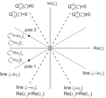
FIG. 1. The regular regions for Jost functionsφ1(X, ζ) in the complexζ-plane. The dashed lines with singularity functions
Q1j(ζ′) determine the boundaries between regular regions. The dotted lines are the lines where the poles appear.
φ1(X,ζ) (as well as 1(X,ζ)). In the general case, it is necessary to take into account both the bound state spectrum and the continuous spectrum. According to the relation (6.20) in Ref.15, the solution of (7) is as follows:
1(X, ζ)=1−
K
k=1 3
j=2
γ1(kj)exp{[λj(ζ
(k) 1 )−λ1(ζ
(k) 1 )]X}
λ1(ζ (k)
1 )−λ1(ζ)
1(X, ωjζ
(k) 1 )
+ 1
2πi
3
j=2
Q1j(ζ′)
exp{[λj(ζ′)−λ1(ζ′)]X}
ζ′−ζ
±
1(X, ωjζ′)dζ′. (11)
Equation (11) contains the spectral data, namelyKpoles with the quantitiesγ1(kj)for the bound state spectrum as well as the functionsQ1j(ζ′) given along all the boundaries of regular regions for the
continuous spectrum. The boundaries between regions, where the Jost functionφ1(X, ζ) is regular, appear at Re(λ1(ζ′)−λj(ζ′))=0 over allj=1 (Ref.15) (see Fig.1). The singularities on boundaries of these regions within the complexζ-plane are taken into account by the third term in the relation (11). The integral in (11) is along all the boundaries (see the dashed lines in Fig.1).
The bound state spectrum is associated with soliton solutions; in this caseQ1j(ζ)≡0 in (11).
The procedure for finding the exactN-soliton solution of the VPE via the inverse scattering method is described in Ref.14. In Sec.III, we study the solutions of the VPE which follow from the continuous part of the spectral data.
III. THE SOLUTIONS ASSOCIATED WITH THE CONTINUOUS PART OF THE SPECTRAL DATA
Now we consider only the continuous spectrum of the associated eigenvalue problem, i.e., we assume that at least some of the functionsQ1j(ζ′) are nonzero, whileγ
(k)
1j ≡0 in Eq. (11). At each
fixedj=1 the functionsQ1j(ζ′) characterize the singularity of 1(X,ζ). This singularity can appear only on boundaries between the regular regions on theζ-plane. The condition Re(λ1(ζ′) − λj(ζ′))
=0 determines these boundaries.15 According to Ref.15, we find that for
1(X,ζ) the complex
ζ-plane is divided into four regions by two lines:
(i)ζ =ω2ξ, where Q(1)12 =0, Q (1) 13 ≡0, (ii)ζ = −ω3ξ, where Q
(2)
12 ≡0, Q (2) 13 =0,
(12)
whereξ is real (see Fig.1). Analysis shows that the direction of the integration in (11) is such that
Let us consider the singularity functionsQ1j(ζ′) on the boundaries, on which the Jost function φ1(X, ζ) is singular, in the form (n=1, 2, ...,N) on the lineζ′=ω2ξ,
Q(1)12(ζ′)= −2πi
N
n=1
q12(2n−1)δ(ζ′−ζ1′),
Q(1)13(ζ′)= −2πiN
n=1
q13(2n−1)δ(ζ′−ζ′ 1)≡0,
(13)
and on the lineζ′= −ω3ξ,
Q(2)12(ζ′)= −2πi
N
n=1
q12(2n)δ(ζ′−ζ2′)≡0,
Q(2)13(ζ′)= −2πiN
n=1
q13(2n)δ(ζ′−ζ′ 2).
(14)
For the singularity functions (13) and (14), the relationship (11) is reduced to the form (M=2N),
1(X, ζ)=1−
M
m=1 3
j=2
q1(mj)exp{[λj(ζ ′
m)−λ1(ζm′)]X} ζ′
m−ζ
× 1(X, ωjζm′). (15)
As follows from the relationship (15) and the formula
φ1X(X, ζ)=
i
√
3[φ1X(X,−ω2ζ)φ1(X,−ω3ζ)
−φ1X(X,−ω3ζ)φ1(X,−ω2ζ)] (16)
given in Ref.14, for example, the singularities in the form (13) and (14) appear in pairsζ2′n−1=ω2ξn,
ζ2′n = −ω3ξn. From (16), considering the limitsζ →ζm′ andX→ − ∞, it also follows immediately
that
q12(2n−1)ω2=q (2n)
13 , with n=1,2, ...,N. (17)
We call attention to the fact that, at the special choice of the singularity functionQ1j(ζ′) for
continuous part of the spectral data as in (13) and (14), the second term on the right-hand side of the relation (15) is similar in mathematical structure to the second term in relation (5.5) from Ref.14. Indeed, the formal substitutionsξm=iξm,q1(mj)=γ
(m)
1j transform the second term in (15) into the
second term in (5.5) from Ref.14. Since there is this transformation, we can apply the procedure developed for solving theN-soliton interaction to obtain the solutions connected with the continuous part of the spectral data for the associated eigenvalue problem.14,15 According to Ref.14(see Eqs. (5.11)– (5.15) therein), we can find 1(X,ζ) and can connect 1(X,ζ) with the solutionW(X), by expanding 1(X,ζ) as an asymptotic series inλ−11(ζ) (see Eq. (5.11) in Ref.14) as follows:
1(X, ζ)=1− 1 3λ1(ζ)
[W(X)−W(−∞)]+O(λ−12(ζ)). (18)
On the other hand, by defining
m(X)=
3
j=2
q1(mj)exp{λj(ζm′)X} 1(X, ωjζm′), (19)
we may rewrite the relationship (15) as
1(X, ζ)=1−
M
m=1
exp{−λ1(ζm′)X} ζ′
m−ζ
063504-5 V. O. Vakhnenko and E. J. Parkes J. Math. Phys.53, 063504 (2012)
From (18) and (20), the following key relationship can be derived (see also Eq. (6.38) in Ref.15):
W(X)−W(−∞)= −3
M
m=1
exp{−λ1(ζm′)X}m(X)
=3 ∂
∂X ln(detM(X)). (21)
HereM(X) is the 2N × 2Nmatrix given by elements
Mml(X)=δml−
3
j=2
q1(mj)exp{[λj(ζ ′
m)−λ1(ζl′)]X} ζl′−ωjζ′
m
. (22)
Now let us consider theT-evolution of the spectral data. By analyzing the solution of Eq. (6) whenX→ − ∞, we find thatφi(X,T,ζ)=exp [−(3λi(ζ))−1T]φi(X, 0,ζ). Hence theT-evolution of the scattering data is given by the relationships (withm=1, 2, ...,M)
qi j(m)(T)=qi j(m)(0) exp{[−(3λj(ζm′)−1
+(3λ1(ζm′))−
1 ]T}, λj(T)=λj(0).
(23)
Consequently, the final result for the solution of the VPE, when we consider the spectral data from the continuous spectrum, as well as taking into account theirT-evolution, is as follows:
W(X,T)=3 ∂
∂X ln (detM(X,T))+const. (24)
The 2N × 2NmatrixM(X,T) is defined as follows:
Mml(X,T)=δml−
3
j=2
q1(mj)(0)exp{[−(3λj(ζ
′ m)−
1
+(3λ1(ζm′))−
1]T
+[λj(ζm′)−λ1(ζl′)]X} ζl′−ωjζ′
m
, (25)
with the relations (n=1, 2, ...,N)
λ1(ζ2′n−1)=ω2ξ2n−1, λ2(ζ2′n−1)=ω3ξ2n−1, q (2n−1)
12 =ω2β2n−1, q (2n−1) 13 =0,
λ1(ζ2′n)= −ω3ξ2n−1, λ3(ζ2′n)= −ω2ξ2n−1, q (2n)
12 =0, q
(2n)
13 =ω3β2n−1. (26)
As will be clear from the examples in Sec.IV, the solution (24) and (25) includeNfrequencies from the continuous part of the spectral data. For this reason, the solution (24) and (25) will be referred to as the N-mode solution of the VPE. Evidently, these discrete modes emanate from the special choice (13) and (14) of the singularity functionsQ1j(ζ′) for continuous part of the spectral data.
For the solution (24) and (25), there areNarbitrary constantsξnandNarbitrary constantsβn.
The constantsξn are real, while the constantsβn, in the general case, are complex. The solution
(24) obtained through the matrix (25) is, in general, a complex function. Consequently, there is a problem in selecting the real solutions from the complex solutions. It turns out that we can obtain the real solutions by means of restriction of arbitrariness in the choice of the constantsβi. For the N-mode solution, we have succeeded in finding these restrictions.
IV. REAL PERIODIC SOLUTIONS OF THE VPE
1. In order to obtain the one-mode solution of the VPE (1), we need first to calculate the 2 × 2 matrixM(X,T) according to (25). For the matrix elementsMkl(X,T), we have
M11 =1−i√ω2β1 3ξ1
exp[−i√3ξ1X+(i
√
3ξ1)−1T],
M12 = −ω23ξβ1
1 exp[2ω3ξ1X+(i
√
3ξ1)−1T],
M21 =ω22ξβ1
1 exp[−2ω2ξ1X+(i
√
3ξ1)−1T],
M22 =1−i√ω3β1 3ξ1
exp[−i√3ξ1X+(i
√
3ξ1)−1T],
(27)
so that its determinant is
detM=1+c1exp(−i
√
3ξ1X+(i
√
3ξ1)−1T)
2
, (28)
wherec1= − iβ1 2√3ξ1
.
As has already been noted, the singularity functions in the form (13) and (14) give rise to a single frequency for the continuous part of the spectral data. Hence, once the expression (28) has been substituted into the key formula (24), (24) must provide us with the one-mode solution.
The condition that WX is real requires a restriction on the constant β1 (if the constantξ1 is arbitrary, but real). We have succeeded in obtaining this restriction (see Appendix), namely that the constant c1, which in general is the complex-valued one c1 = |c1|exp (iχ1), should possess unit modulus |c1| = 1, while the arbitrary real constant χ1 defines an initial shift of solution
X1=χ1/(
√
3ξ1) so that
detM =
1+exp
−i√3ξ1(X−X1)+
T
i√3ξ1
2
. (29)
The final result for one mode of the continuous spectrum is the solution (24) with (29), namely,
W = −3√3ξ1tan
√
3
2 ξ1(X−X1)+
T
2√3ξ1
+const. (30)
The corresponding solution forU =WX (withUgoverned by (4)) was obtained recently by
other methods, for example, by the sine-cosine method,17the (G′/G)-expansion method,13 and the extended tanh-function method.17–19However, only the approach developed here and the solution in the form (24) and (25) enable us to study the interaction the periodicN-mode waves.
2. Let us consider the two-mode solution of the VPE. In this caseM(X,T) is a 4 × 4 matrix. We will not give the explicit form of this matrix here, but we find its determinant
detM(X,T)=(1+q1+q2+b12q1q2)2, (31) where
qi =ciexp[−i
√
3ξiX+(i
√
3ξi)−1T], ci = −
iβi
2√3ξi ,
b12 =
ξ
2−ξ1
ξ2+ξ1
2 ξ2 1 +ξ
2 2 −ξ1ξ2
ξ2 1 +ξ
2 2 +ξ1ξ2
, b12 ≥0. (32)
In Appendix, the restrictions on the constantsci= |ci|exp (iχi) for real solutions are found. The real
constantsχidefine the initial shifts of solutionsXi =χi/(
√
3ξi). The analysis in considerable detail
shows (see Appendix) that the relations|c1| = |c2| =1/
√
b12are sufficient conditions in order that
Wmay become real. Consequently, the real solution describing the interaction of two periodic waves for the VPE is defined by the key relationship (24), where
detM(X,T)=
1+√1
b12
q1+ 1
√
b12
q2+q1q2
2
063504-7 V. O. Vakhnenko and E. J. Parkes J. Math. Phys.53, 063504 (2012)
andb12is as in (32), whileqishould contain the phase shiftsXi =χi/(
√
3ξi) as in (34), namely
qi =exp
−i√3ξi(X−Xi)+(i
√
3ξi)−1T. (34)
3. ForN=3 in relationship obtained from (25)
detM(X,T)=(1+c1q1+c2q2+c3q3+c1c2b12q1q2
+c1c3b13q1q3+c2c3b23q2q3
+c1c2c3b12b13b23q1q2q3)2 (35)
withqi,cias in (32) and
bi j =
ξ
j−ξi ξj+ξi
2ξ2
i +ξ
2
j −ξiξj ξ2
i +ξ
2
j +ξiξj
, bi j =bj i, (36)
we writeci = |ci|exp (iχi), then the argumentsχi determine the initial phase shifts of mode Xi
=χi/(
√
3ξi). As is proved in Appendix, the conditions on the constantsc1(or the same onβi) are
|c1| =1/
b12b13, |c2| =1/
b12b23, |c3| =1/
b13b23. (37)
Hence, the three-mode solution is the relation (24) with
detM =
1+√ 1
b12b13
(q1+q2q3)+ 1
√
b12b23
(q2+q1q3)
+√ 1
b13b23
(q3+q1q2)+q1q2q3
2
. (38)
Here the phase shiftsXiare taken into account inqiby way of (34).
4. ForN=4 the restrictions are as follows (see Appendix):
|ci| =
4
j=i b−
1 2
i j , bi j =bj i, i =1,2,3,4. (39)
The determinant for a real solution (24) is as follows:
detM =
1+√ 1
b12b13b14
(q1+q2q3q4)
+√ 1
b12b23b24
(q2+q1q3q4)
+√ 1
b13b23b34
(q3+q1q2q4)
+√ 1
b14b24b34
(q4+q1q2q3) (40)
+√ 1
b13b14b23b24
(q1q2+q3q4)
+√ 1
b12b14b23b34
(q1q3+q2q4)
+√ 1
b12b13b24b34
(q1q4+q2q3)+q1q2q3q4
2
.
V. CONCLUSION
We have adapted and applied the inverse scattering method to the Vakhnenko-Parkes equation in order to find the solutions that are associated with the continuous spectrum of the spectral problem. The special form of the singularity function for continuous part of the spectral data enabled us to obtain the multi-mode solutions. The sufficient conditions have been proved in order that the solutions become real functions. We have described how to define the interaction of the multi-mode periodic waves. The procedure has been illustrated by considering a number of examples.
ACKNOWLEDGMENTS
V.O.V. is grateful to K. P. Kutsevol for stimulating criticism and helpful discussions.
APPENDIX: THE CONDITIONS ON THE CONSTANTSciFOR REAL SOLUTIONS
We use the caseN=4 as an example to prove the restrictions on the constants, at which the so-lutionW(X,T) is real. We will consider the auxiliary function f =√detM(X,T) for convenience, namely
f =1+c1q1+c2q2+c3q3+c4q4+c1c2b12q1q2
+c1c3b13q1q3+c1c4b14q1q4+c2c3b23q2q3
+c2c4b24q2q4+c3c4b34q3q4+c1c2c3b12b13b23q1q2q3
+c1c2c4b12b14b24q1q2q4+c1c3c4b13b14b34q1q3q4
+c2c3c4b23b24b34q2q3q4
+c1c2c3c4b12b13b14b23b24b34q1q2q3q4. (A1)
We here redefine the valuesci= |ci|, since the argumentsχican always be introduced in the variables qi=exp (iθi) withθ = −
√
3ξi(X−Xi)−(
√
3ξi)−1T. The solution (21) then has a form
W(X,T)=6 ∂
∂X ln(f)+const. (A2)
The functionfis complex-valued, i.e.,
f = fRe+ifI m = |f|exp(iχf), fRe=Re(f),
fI m =Im(f), tan(χf)= fI m/fRe, (A3)
hence,
W(X,T)/6= ∂
∂X ln(|f|)+i ∂χf
∂X +const. (A4)
If we succeed in making∂2χ
f/∂X2≡0 by the choice of the constantsci, then the solutionW(X,T)
063504-9 V. O. Vakhnenko and E. J. Parkes J. Math. Phys.53, 063504 (2012)
Let us writefImandfRein explicit forms
fI m =c1sin(θ1)+c2sin(θ2)+c3sin(θ3)+c4sin(θ4)
+c1c2b12sin(θ1+θ2)+c1c3b13sin(θ1+θ3)
+c1c4b14sin(θ1+θ4)+c2c3b23sin(θ2+θ3)
+c2c4b24sin(θ2+θ4)+c3c4b34sin(θ3+θ4)
+c1c2c3b12b13b23sin(θ1+θ2+θ3) (A5)
+c1c2c4b12b14b24sin(θ1+θ2+θ4)
+c1c3c4b13b14b34sin(θ1+θ3+θ4)
+c2c3c4b23b24b34sin(θ2+θ3+θ4)
+c1c2c3c4b12b13b14b23b24b34sin(θ1+θ2+θ3+θ4),
fRe=1+c1cos(θ1)+c2cos(θ2)+c3cos(θ3)+c4cos(θ4)
+c1c2b12cos(θ1+θ2)+c1c3b13cos(θ1+θ3)
+c1c4b14cos(θ1+θ4)+c2c3b23cos(θ2+θ3)
+c2c4b24cos(θ2+θ4)+c3c4b34cos(θ3+θ4)
+c1c2c3b12b13b23cos(θ1+θ2+θ3) (A6)
+c1c2c4b12b14b24cos(θ1+θ2+θ4)
+c1c3c4b13b14b34cos(θ1+θ3+θ4)
+c2c3c4b23b24b34cos(θ2+θ3+θ4)
+c1c2c3c4b12b13b14b23b24b34cos(θ1+θ2+θ3+θ4).
Now we select a factor sin(12(θ1+θ2+θ3+θ4)) from fIm and a factor cos(12(θ1+θ2+θ3+θ4)) fromfRe. This can be done if the following conditions are satisfied:
c1=c2c3c4b23b24b34, c2=c1c3c4b13b14b34,
c3=c1c2c4b12b14b24, c4=c1c2c3b12b13b23,
c1c2b12=c3c4b34, c1c3b13=c2c4b24, c1c4b14=c2c3b23,
c1c2c3c4b12b13b14b23b24b34=1. (A7)
It turns out that all these relations are valid, when
c1= 1
√
b12b13b14
, c2= 1
√
b12b23b24
,
c3= 1
√
b13b23b34
, c4= 1
√
b14b24b34
. (A8)
The conditions (A8) enable us to reduce bothfImandfReto the forms
fI m =2gsin(12(θ1+θ2+θ3+θ4)),
where
g = √ 1 b12b13b14
cos12(θ1−θ2−θ3−θ4)
+√ 1
b12b23b24 cos1
2(θ2−θ1−θ3−θ4)
+√ 1
b13b23b34 cos1
2(θ3−θ1−θ2−θ4)
+√ 1
b14b24b34
cos12(θ4−θ1−θ2−θ3) (A10)
+√ 1
b13b14b23b24 cos1
2(θ1+θ2−θ3−θ4)
+√ 1
b12b14b23b34 cos1
2(θ1+θ3−θ2−θ4)
+√ 1
b12b13b24b34
cos12(θ1+θ4−θ2−θ3) .
Now it is readily seen from (A3) that
χf = 12(θ1+θ2+θ3+θ4) (A11)
and as a consequence we have
∂2χf ∂X2 =
∂2χf
∂X∂T =0. (A12)
Hence, as follows from (A4), the four-mode solution of the VPE can be reduced to real form with four real constantsXiand four real constantsξi(see (41)).
Without proof here we give the following conditions on the constants ci that ensure the real N-mode solution of the VPE:
|ci| = N
j=i b−
1 2
i j , bi j =bj i, i =1, ..., N, (A13)
whereas theNconstantsξidetermine the valuesbijand theNconstantsXithroughβidefine the phase
shifts of the separate modes. Note that these relations are sufficient conditions, but not necessary ones.
1R. Hirota,The Direct Method in Soliton Theory(Cambridge University Press, 2004). 2A. M. Wazwaz,Phys. Scr.82, 065006 (2010).
3M. J. Ablowitz and H. Segur,Solitons and the Inverse Scattering Transform(SIAM, 1981).
4B¨acklund Transformations, the Inverse Scattering Method, Solitons, and Their Applications, edited by R. M. Miura
(Springer, 1976).
5S. P. Novikov, S. V. Manakov, L. P. Pitaevskii, and V. E. Zakharov,Theory of Solitons: The Inverse Scattering Methods
(Plenum, 1984).
6V. A. Vakhnenko,J. Phys. A25, 4181 (1992).
7E. J. Parkes,J. Phys. A26, 6469 (1993).
8V. O. Vakhnenko,J. Math. Phys.40, 2011 (1999).
9V. O. Vakhnenko and E. J. Parkes,Nonlinearity11, 1457 (1998).
10A. J. Morrison, E. J. Parkes, and V. O. Vakhnenko,Nonlinearity12, 1427 (1999).
11M. L. Gandarias and M. S. Bruz´on, “Symmetry reductions and exact solutions for the Vakhnenko equation,” inProceedings
of XXI Congreso de Ecuaciones Diferenciales y Aplicacions, XI Congreso de Matim´atica Aplicada, Ciudad Real, 21-25 Septiembre 2009, pp. 1–6.
12P. G. Est´evez,Theor. Math. Phys.159, 762 (2009).
063504-11 V. O. Vakhnenko and E. J. Parkes J. Math. Phys.53, 063504 (2012)
14V. O. Vakhnenko and E. J. Parkes,Chaos, Solitons Fractals13/9, 1819 (2002). 15P. J. Caudrey,Physica D6, 51 (1982).
16D. J. Kaup, Stud. Appl. Math.62, 189 (1980).
17E. Yusufoglu and A. Bekir,Chaos, Solitons Fractals38, 1126 (2008).
18E. J. Parkes,Appl. Math. Comput.217, 3575 (2010).