Assessing parameter uncertainty on coupled models using
minimum information methods
Tim Bedforda, Kevin J Wilsona,∗, Alireza Daneshkhahb
a
Department of Management Science, University of Strathclyde, Glasgow, G1 1QE, UK b
Cranfield Water Science Institute, Cranfield University, Vincent Building, Cranfield, Bedford, MK43 0AL
Abstract
Probabilistic inversion is used to take expert uncertainty assessments about observable model outputs and build from them a distribution on the model parameters that captures the uncertainty expressed by the experts. In this paper we look at ways to use minimum information methods to do this, focussing in particular on the problem of ensuring con-sistency between expert assessments about differing variables, either as outputs from a single model, or potentially as outputs along a chain of models. The paper shows how such a problem can be structured and then illustrates the method with two examples; one involving failure rates of equipment in series systems and the other atmospheric dispersion and deposition.
Keywords: Minimum information, coupled models, expert judgement, Probabilistic Risk Analysis, Gaussian plume.
1. Introduction
An important element of Probabilistic Risk Analysis is assessment of uncertainty in model outputs. Physical models do not perfectly represent the phenomena they are meant to describe for many reasons: lack of complete understanding of the physical phenomena, deliberate simplifications in the model (for example, because of the need to run the model quickly), inadequate choice of model parameters, and so on.
Bedford and Cooke [1] stress the importance of assessing uncertainties for observable quantities when using probability. Since it is typically model outputs that are observ-able quantities, and many model parameters are not directly observobserv-able (maybe having no direct physical interpretation) it is therefore necessary to consider ways of taking probability distributions that describe the uncertainty in model output quantities and “back-fitting” these to generate a distribution on the model parameters so that this matches the uncertainty specified for the output parameters in the following sense: If we randomly choose a set of model parameters and compute the model outputs then those
∗Corresponding author, tel: +44 141 548 4578, fax: +44 141 552 6686
Email addresses: [email protected](Tim Bedford),[email protected]
(Kevin J Wilson),[email protected](Alireza Daneshkhah)
outputs are also random. The distribution of the outputs obtained is called the push-forward of the distribution on the model parameters and should match the uncertainty for the observable quantities.
The problem of Probabilistic Inversion (PI) is simply the problem of computing a distribution on the model parameters with the property that its push forward matches that specified for the distribution on the observable quantities. See Bedford and Kraan [2] and Kurowicka and Cooke [3] for different approaches to this problem. Having defined an uncertainty distribution on the the model parameters, this then allows us to make predictions, incorporating our uncertainty, on model outputs for any set of model inputs. The probabilistic inversion problem is typically either under- or over-specified. This means that the constraints imposed by the output distributions are either not sufficiently strong to lead to a single solution to the PI problem, or they are mutually contradictory, and give rise to an infeasible problem.
Previous approaches have used minimally informative distributions to solve the prob-lem of under-specification, and have either ignored the probprob-lem of infeasibility or used slightly ad-hoc approaches to deal with it. This paper develops the ideas proposed in Bedford [4] to use minimum information methods [5, 6] to provide guidance in the specifi-cation of constraints that are not infeasible. It also gives a method to map out the feasible region for the constraints. Minimum information methods use constraints on expected values rather than quantile information, though we discuss how quantile information can be incorporated.
The paper generalizes the context given above to one of “coupled” models, that is, the situation where we have several models which are sequentially linked in the sense that the outputs of the first are the inputs of the second, and so on. Hence specifications may be made of distributions of input and output parameters, and the distributions on the model parameters are supposed to push forward to these.
The main contribution of this paper is therefore to show how the minimum infor-mation approach can be used to generate solutions to the PI problem in the context of coupled models. The rest of the paper is structured as follows. In Section 2 we provide the mathematical setup to the problem, considering coupled models and minimum in-formation modelling. In Section 3 we outline the solution to the continuous PI problem for coupled models and in Section 4 we give the equivalent solution to the discretized problem. Section 5 investigates the specification of feasible constraints for the coupled PI problem and considers the effect of fixing the constraints. In Sections 6 and 7 we provide two examples; the first considering the failure rates of machines located in series and the second based on the dispersion and deposition problem considered by Kraan in [7]. Finally, in Section 8, we give some conclusions and a discussion of areas for further work.
2. Mathematical set up
2.1. Coupled models
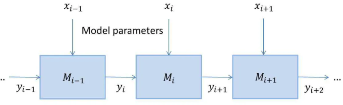
We consider modelsMi taking input parametersyi and giving output parametersyi+1.
Figure 1: A diagram illustrating the form of coupling of models.
illustration of this situation is given in Figure 1.
Some of the parameters may be directly measurable. Some we might be able to choose. However, often the model parameters are not known directly and we have to infer them, or infer uncertainty distributions over them. The inputs and outputs of the models are observable quantities in principle, and we may therefore be able to use expert judgement to assess distributions or expected values. In probabilistic inversion we try to find a distribution for the parameters that matches (when propagated through the model) the distributions specified by the experts for the observable quantities.
As noted above, the PI problem is typically either over- or under-constrained. Over-constraint happens because the quantities to be assessed are typically functionally related through the model, so it easy for experts to provide information on observables that is mutually inconsistent (assuming the model is correct). Under-constraint happens because there is consistency but there is still not enough information to uniquely determine the distribution on the parameters. In our approach we use a minimum information property to solve the problem of under-constraint, and a sequential approach to expert elicitation to avoid the problem of over-specification.
2.2. Minimum Information Modelling
Suppose we have continuous random variableX, which could be multi-dimensional, and two densities,f1(·) andf2(·). Then the relative information off1(·) tof2(·) is a measure
of how similar the two distributions are. It is defined as
I(f1|f2) =
Z
f1(x) log
f
1(x)
f2(x)
Iff1(·) =f2(·) then the relative information is zero. It then increases as the deviation
between the two distributions becomes greater.
In the problems considered in this paper we wish to find the distribution,f1(·), which
has minimum information, with respect to the background distributionf2(·), subject to
some real valued functions h1. . . , hk taking expectations α1, . . . , αk. These are known as theconstraints. The choice of background distribution is an important consideration as this specifies whatf1(·) should look like in the absence of more specific information.
Typical choices might be the uniform, log-uniform and Normal distributions (but this can be subject to sensitivity analysis as we discuss later).
The minimum information distribution is therefore, in some sense, the “simplest” dis-tribution which satisfies the required criteria. If, relative to the background disdis-tribution, this distribution exists then it is unique and takes the form, Lanford [8],
f(x) =
expnPk
i=1λihi(x)
o
Z(λ) , (1)
for Lagrange multipliersλ= (λ1, . . . , λk) (depending onα1, . . . , αk), whereZ(λ) is the
normalising constant. An important contribution of this paper is a procedure which provides a method of specifying the constraints using expert elicitation which ensures such a unique minimally informative solution exists. We can approximate this density arbitrarily well using discrete densities
p(xj)∝exp
( k
X
i=1
λihi(xj)
)
, (2)
wherexj, j = 1, . . . , n is a suitable discretization of x. A derivation of these results is outlined in Bedford and Wilson [9].
We see that, for minimum information problems, constraints are naturally specified as expectations on functions of the parameters. We can incorporate quantile assessments as the expert judgement by specifying the hi’s as indicator functions in terms of the quantile functions of the parameters. An example is given in Bedfordet al[10] and the technique is used in the failure rates example in Section 6.
We shall now consider how to evaluate the feasible values of constraints when the specifications of those constraints are made sequentially. Initially we consider the con-tinuous problem.
3. The Continuous Problem
Consider a collection of parameters from a deterministic model or sequence of models, denotedX. In generalX could have a large number of dimensions. Suppose that expert elicitation results in the specification of the expectations of some functions,h1, . . . , hp, of
these parameters, denotedα1, . . . , αp. These are the constraints in the problem. We wish
to find the distribution with minimum information which satisfies these expectations. As we saw in the previous section this minimum information distribution has a density atxwhich is proportional to
exp
( p
X
i=1
λihi(x)
)
for some parametersλ1. . . , λp. We can define the functionφ:Rp→Rp so thatφgives
the expected values obtained from choosing the minimum information distribution with parametersλ1, . . . , λp. That is,
φ(λ1. . . , λp) = (α1, . . . , αp).
In particular,
φ(λ1, . . . , λp) =
Rh
1(x) exp{Piλihi(x)}dx
R
exp{P
iλihi(x)}dx
,· · · ,
R
hp(x) exp{P
iλihi(x)}dx
R
exp{P
iλihi(x)}dx
.
The functionφis invertible and has good analytical properties.
We wish to specifyα1and use this to explore the possible valuesα2can take. Having
done this the next step is to find the possible values for α3 having specified α1, α2.
We can continue in this way, evaluating the possible specifications of each expectation consistent with previously specified values, until all of the required expectations have been set. Doing this stepwise allows us to guide the expert in making allowable choices for the constraints.
To see how this can be achieved, initially consider functionsψ1, ψ2, . . . , ψp which are defined, in terms ofφ= (φ1, . . . , φp), as
ψ1(λ1) = φ1(λ1,0, . . .),
ψ2(λ1, λ2) = (φ1(λ1, λ2,0, . . .), φ2(λ1, λ2,0, . . .)),
and so on. Since eachφiis monotone,ψ1, ψ2, . . . , ψpare monotone. Thereforeψ1, ψ2, . . . , ψp are invertible and so we can invertψ1to obtainψ1−1. This allows us to calculateλ1from
a givenα1, for example using Newton’s method. We can also use this relationship to
explore the possible values ofα1.
Having specified α1 =α∗1 we would like to find the values of λ1, λ2 for a particular
α2. That is, we are interested in
ψ−1
2 |α1=α∗1 (α2) = (λ1, λ2). (3) Thus we are mapping image(ψ2)∩ {α1 = α∗1} → R2. This is a map of one variable.
Initially, having specifiedα1=α∗1, we can identify a value ˜α2so that
ψ−1
2 |α1=α∗1 (˜α2) =
λ(1)1 ,0
,
by taking ˜α2 = E[h2(X)] under the distribution with parameters (λ(1)1 ,0). We can use
this as a starting value for exploring the range of possible values forα2. The range can
then be explored using the inverse function in (3). Having found the set of feasible values we specify the value ofα2=α∗2 in this range and useψ−21as above to find (λ
(2) 1 , λ
(2) 2 ).
The general step begins with the specification of α1 =α∗1, . . . , αn−1 =α∗n−1 having
been made. The relevant conditional mapping is then
ψ−1
n |α1=α∗1,...,αn−1=α∗n−1(˜αn) =
λ(n−1)
1 , . . . , λ (n−1) n−1 ,0
.
This is used to explore the space of possible values forαn. Having specifiedαn=αn∗ we use it to calculate (λ(1n), . . . , λ(nn)). We see thatλ(
j)
It is clear from the above formulation that the order the specifications are made is going to have an effect as we are considering expectations one at a time. This is discussed in Section 7.3. To solve such problems in practice we work with the discrete version of the problem. This is set out in the next section.
4. The discretized problem
Suppose we have discretized at points x1, . . . , xm. In two dimensions these could be
points on the square. As before we have constraints on some functionsh1, . . . , hp in the form of expected valuesα1, . . . , αp. The minimum information distribution has mass at
pointxj which is proportional to exp(Piλihi(xj)).
We replace integrals by sums in the definition ofφ. That is,
φ(λ1, . . . , λp) =
P
jh1(xj) exp{
P
iλihi(xj)}
P
jexp{
P
iλihi(xj)}
, . . . ,
P
jhp(xj) exp{Piλihi(xj)}
P
jexp{
P
iλihi(xj)}
!
.
Now, since we have a simple, analytic formula forφ, we can determineDφ, the matrix of derivatives with respect to theλ’s. This is ap×pmatrix with elements
∂φk
∂λl =
P
jhk(xj)hl(xj)Aj
P
jAj
−[
P
jhk(xj)Aj]×[Pjhl(xj)Aj] [P
jAj]2
,
where Aj = exp{Piλihi(xj)}. As long as Dφ is of full rank then we can invert it, numerically, to obtain the matrix of derivatives with respect to theαk’s.
This enables us to work out, to first order, using Newton’s method for example, how the Lagrange multipliers change when we keepα1, . . . , αk−1fixed, and changeαkslightly. When we approach the boundary of the convex set of possibleαk values, the Lagrange multipliers go to plus or minus infinity.
This enables us to work out which parameter vector gives a particular constraint vector. Hence we can systematically map out the ranges of allowed expectations as follows.
1. With the first function h1 we take λ1 = ±N, where N is some large number, to
obtain upper and lower bounds onα1.
2. The expert chooses α1. We calculate, numerically by inversion, what the
corre-spondingλ1 is, denotedl1.
3. For the next function h2 we take λ1 = l1 and λ2 = 0. This means that our
starting value forα2 is whatever we had for the expectation value with respect to
the minimum information distribution we used in Step 1.
4. Using this as a starting value forα2we increaseα2, keepingα1fixed, and work out
the corresponding values of λ1 and λ2 using (Dφ)−1. When λ1, λ2 become large
we have reached the largest feasibleα2.
5. We repeat Step 4 decreasingα2 from its initial value.
We shall illustrate this methodology by applying it to two examples; the first a model of atmospheric dispersion and dispersion and the second a model assessing the failure rates of machines in series. However, first we consider the mapping out of the feasible regions for multiple constraints.
5. Investigation of the feasible region for the constraints
We can investigate the convex set of possible combinations of different constraints known as the feasible region. To do so consider the normalising constant from (1). It is
Z(λ) =
Z
exp
( X
i
λihi(x)
)
dx,
for vectorxand parametersλ= (λ1, . . . , λp). Taking logs and differentiating with respect
to Lagrange multiplierλi recovers the expectations defined previously,
d dλi
logZ(λ) =
R
hi(x) exp{P
iλihi(x)}dx
R
exp{P
iλihi(x)}dx
= Eλ[hi(x)].
If we differentiate a further time with respect to the sameλi we obtain the variance of the constraint function associated with this expectation,
d2
dλ2
i
logZ(λ) =
R
h2
i(x) exp{
P
iλihi(x)}dx
R
exp{P
iλihi(x)}dx
−
Rhi(x) exp{P
iλihi(x)}dx
R
exp{P
iλihi(x)}dx
2
= Varλ(hi(x))≥0.
Let us define the function g to be the vector of the constraint functions, so that g = (h1(x), . . . , hp(x)). Then the expectation ofgis simply Eλ[g] = (Eλ[h1(x)], . . . ,Eλ[hp(x)]).
If we make the assumption thatg is bounded then Eλ[g] is also bounded. We know that there is a uniqueλassociated with any possibleαin the convex hull ofg. We also see that each expectation Eλ[hi(x)] is increasing as λ increases. This will allow us to map out the feasible region of Eλ[g].
Considerλ1. . . , λpin the sphere of radius 1, p
X
i=1
λ2
i ≤1. (4)
If we take as our starting point the sphere with unit radius defined by (4) this will map out a region of values, corresponding to thisλ, for Eλ[g]. If we then multiply the vector (λ1, . . . , λp) by somer >1, so that we have r×(λ1, . . . , λp), we are now in the sphere
defined by
p
X
i=1
(rλi)2≤r2.
That is, we are moving outward in a radial direction. From this we obtain a new, larger, region for Eλ[g]. As r becomes large this region will tend to the overall feasible region for Eλ[g].
Table 1: The possible outcomes, background distribution and contributions to the MI solution for the coin tossing example.
{X, Y} 0,0 0,1 1,0 1,1 Background dist. 1/4 1/4 1/4 1/4
eλihi(x,y) 1 1 eλ1 eλ1+λ2
5.1. Coin tossing example
Suppose we have two coins and that we suspect that each is biased. LetX, Y represent one realisation for each coin of a single toss. That is,
X, Y =
(
1, if heads,
0, if tails,
with probabilitiespX, pY. We also suspect that the tosses are not independent. Further suppose that the functions we are going to ask an expert to specify areh1=xandh2=
xy. We know the form of the minimum information distribution in this case. A sensible measure to take as the background distribution would appear to be (1/4,1/4,1/4,1/4) on the four different possible outcomes of the two tosses.
Table 1 sets out each of the outcomes, the associated background distribution and the minimum information terms found analytically. From this we can calculateZ(λ). It is
Z(λ) = 1 4(2 +e
λ1+eλ1+λ2).
If we take logarithms then differentiate we obtain the expectations of each of the func-tions. They are
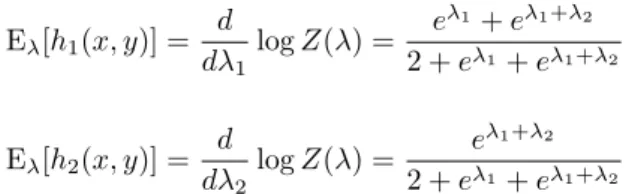
Eλ[h1(x, y)] =
d dλ1
logZ(λ) = e
λ1+eλ1+λ2 2 +eλ1+eλ1+λ2, and
Eλ[h2(x, y)] =
d dλ2
logZ(λ) = e λ1+λ2 2 +eλ1+eλ1+λ2.
We can use these equations to map out the feasible region for the expectation of g = (h1(x, y), h2(x, y)). We begin with r = 1 and then increase it gradually up tor = 10.
The results are given in Figure 2 for r = 1,2,3,10. We see that, as r increases, the region becomes larger until, whenr= 10, it is covering the entire feasible region for g. Some pseudo-code illustrating how to explore the feasible region in this way is given in Algorithm 1 in the Appendix.
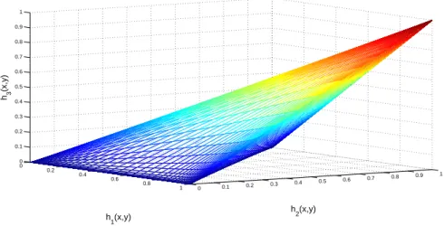
We can also carry out such an investigation in 3 dimensions. Suppose thatX, Y are defined as above but now we are interested in the expectations associated with three functions, namely
h1(x, y) =x, h2(x, y) =y, h3(x, y) =xy.
We can apply the methodology as above. The functionZ(λ) is now given by
Z(λ) =1 4(1 +e
λ1 +eλ2
0 0.1 0.2 0.3 0.4 0.5 0.6 0.7 0.8 0.9 1 0
0.1 0.2 0.3 0.4 0.5 0.6 0.7 0.8 0.9 1
h
1(x,y) h2
(x,y)
Figure 2: The feasible region for the expectation ofggivenr= 1,2,3,10.
Taking logarithms and differentiating we can find the expectations of the three functions of interest. They are
Eλ[h1(x, y)] = e
λ1+eλ1+λ2+λ3 1 +eλ1+eλ2+eλ1+λ2+λ3,
Eλ[h2(x, y)] = e
λ2+eλ1+λ2+λ3 1 +eλ1+eλ2+eλ1+λ2+λ3, and
Eλ[h3(x, y)] =
eλ1+λ2+λ3
1 +eλ1+eλ2+eλ1+λ2+λ3.
We can then use these three expressions to evaluate the convex region associated with a sphere in (λ1, λ2, λ3) of radius 1 and expand this, moving outwards along the radius,
until we are satisfied we are evaluating the entire feasible region for the three constraints. A plot of this, for a radiusr= 10, is given in Figure 3.
5.2. The discretized case
As, in practice, we usually solve the minimum information problem in a discretized version of the parameter space we now consider such a discretized space in the context of exploring the feasible region of Eλ[g]. In this case the quantityZ(λ) is
Z(λ) =X j
exp
( X
i
λihi(xj)
)
,
and the expectation ofhi(x) is
Eλ[hi(x)] = d
dλi
logZ(λ) =
P
jhi(xj) exp{
P
iλihi(xj)}
P
jexp{
P
iλihi(xj)}
0 0.2
0.4 0.6
0.8
1 0 0.1 0.2 0.3 0.4 0.5 0.6 0.7 0.8 0.9 1 0
0.1 0.2 0.3 0.4 0.5 0.6 0.7 0.8 0.9 1
h
2(x,y)
h
1(x,y) h3
(x,y)
Figure 3: The feasible region for the expectation ofgin the three dimensional example.
We then proceed, evaluating the feasible region beginning on a sphere of radius 1 and moving outwards in a radial direction, in the same manner as in the continuous case.
5.3. Fixed constraints
Suppose we have two constraints,α1 and α2. Let us further suppose that we fixα2 for
all time at some value ˜α2. What effect does this have? Consider the mappingφ, in terms
ofZ(λ1, λ2), as
φ:
d dλ1
logZ(λ1, λ2), d
dλ2
logZ(λ1, λ2)
.
Fixingα2= ˜α2 is equivalent to fixing
d
dλ2logZ(λ1, λ2) = ˜α2. (5)
Now, when we considerα1, which is given by
d dλ1
logZ(λ1, λ2) =α1,
it is a function of bothλ1 and λ2. However, (5) has fixed the relationship betweenλ1
andλ2 and so λ1 is now an implicit function of λ2. Thus α1 is now a function of one
variable, and any value it takes will be “on the curve” betweenλ1andλ2implied by (5).
6. Example: Failure rates of machines in series
Suppose we have two machines,M1, M2, which are physically co-located and, within a
larger process, are to be used in series. In this sense the two machines are then coupled as the physical outputs of one machine will become the physical inputs of the next machine. Suppose we are interested in the failure rates of the two machines,λ1(t), λ2(t)
respectively. In particular, we wish to evaluate the uncertainty distributions over the failure rates of the machines. It would seem reasonable that the failure rates,λ1(t), λ2(t),
would not be statistically independent as a result of the coupled nature of the machines and their physical co-location. For example, if it were not built into the modelling process elsewhere, an extreme weather event at the location of the machines would likely cause both to fail. This would result in the failure rates of the machines being correlated.
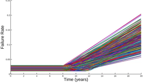
A simple model for the failure rate of machines which captures a constant failure rate due to random failures for a proportion of the lifetime of a machine or component and an increasing failure rate as a result of degradation beyond a certain age was proposed by van Gestel [11]. An illustration of the form of the model is given in Figure 4.
Figure 4: A simple model for the failure rate of machineiincorporating three parameters, (Hi, Ti, θi).
In Figure 4 we see that the model contains three parameters, (Hi, Ti, θi). An ad-vantage of the model is that each of the parameters has an intuitive meaning;Hi is the failure rate of machineiunder purely random failures, Ti is the time at which machine
with a negative gradient prior to the constant random failures section. This would add two additional parameters to the model, the changepoint time between early life and random failures and the angle of the gradient in early life. However, for this illustrative example, we shall consider the simpler three-parameter model.
If we return to the coupled machines we see that we have 6 parameters in total and so our parameter set isx= (H1, T1, θ1, H2, T2, θ2). The changepoint time parameter of
the first model,T1, is an observable quantity and so an expectation on it can be elicited
directly and will not affect the inference on the other parameters in the model. We could also ask experts about their expectation on the probability that the first failure of machine 1 was afterT1. This is given by the expectation of Pr(t > T1) = exp{−H1T1}.
We discuss how to elicit such quantities in Section 6.1. Thus, the first two constraints on machine 1 are given by
h1,1(x) =T1, h1,2(x) = exp{−H1T1}.
We would also like to elicit some information concerningθ1in order that we can evaluate
the uncertainty on all of the machine 1 parameters. We can do so by asking the expert to assess the expected probability that machine 1 will have failed in the first year after it enters the ageing state. That is, we evaluate the expectation of Pr(t < T1+ 1| t ≥
T1) = [R(T1)−R(T1+ 1)]/R(T1). This gives the third constraint as
h1,3(x) =
exp{−H1T1} −exp
−H1T1−
1
2(H1+ tanθ1)
exp{−H1T1}
=
1−exp
−1
2(H1+ tanθ1)
.
It is clear that the specification of the first constraint will affect the possible values for the second and third constraints and so it will be important to perform the steps sequentially as in the previous example. We can also ask the expert to specify the same values for machine two giving three further constraints;
h2,1(x) =T2, h2,2(x) = exp{−H2T2},
h2,3(x) = exp{−H2T2}
1−exp
−1
2(H2+ tanθ2)
.
As the failure rates of the machines will not, in general, be statistically independent, we are also interested in the joint behaviour of the different elements of the failure rates. To consider the correlations between the different elements we shall define a further constraint function relating parameters of the two machines. This is simply the probability that the difference between the times the two machines start ageing is less than one year. To define this probability we set the constraint equal to the indicator function for the event of interest. That is,
h(1,2),1(x) =
(
1, if|T1−T2|<1,
6.1. Eliciting failure rate information from experts
The elicitation of expert judgements for probabilistic models should always be carried out on observable quantities [12, 1]. In the case of the failure rate model for machines considered here it is not reasonable to elicit information from experts about expectations on the failure rates directly. When he proposed the model, van Gestel [11] elicited information for a single machine from experts by asking them for the changepoint time between random failures and ageingTi, the percentage of random failures per time period
Hi and the mean time to failure.
Our minimum information approach differs as it is specified in terms of expected values. Our first proposed constraint for each machine is the expectation of the change-point time between random failures and the start of ageing. It is felt that engineers with experience of observing the failure behaviour of large numbers of similar machines over long time periods would be comfortable with this. The second constraint we have used for each machine is the expected probability that the first failure of the machine is after ageing starts. This is observable in the sense that the expert could be asked to specify this as the average proportion of machines which would not fail in this time over very large datasets. The third constraint for each machine, the expected probability that the machine will have failed a year after entering the ageing state given that it had not failed up to this time, can be elicited in a similar way.
The constraint which considers the relationship between failures in the two models is of a different form to the other constraints. Rather than asking the expert for an expected value directly, it instead asks the expert for a probability found as the expectation of an indicator variable. This probability is that ageing in the two machines begins less than a year apart. This is an observable quantity as the point at which a machine starts ageing is observable.
6.2. Simulating from the minimum information distribution
Making specifications on these 7 constraint functions sequentially will uniquely determine the minimum information distribution over the parameters of the failure rate functions for the two machines. Let us denote this distributiong(x). We can then simulate from this distribution which gives us uncertainty distributions on the two failure rates of the machines. To do so we apply the following steps.
• Sample a uniform random variableu= (u1, . . . , u6), whereui ∼U(0,1).
• A sample from the MI distribution, ˜x, can then be found. The first sampled parameter is ˜x1 = G−11(u1), where G−11(·) is the inverse cumulative distribution
function ofx1. The rest of the parameters are then sampled sequentially as
˜
xi=G−i 1(ui|x˜1, . . . ,x˜i−1),
whereG−1
k (· | ·) is the relevant one dimensional, conditional, cumulative distribu-tion funcdistribu-tion.
• This gives one realisation ofλ1(t) andλ2(t), the failure rates of the two machines.
• Repeat this a large number of times which gives uncertainty distributions onλ1(t)
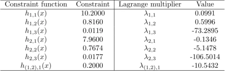
Constraint function Constraint Lagrange multiplier Value
h1,1(x) 10.2000 λ1,1 0.0991
h1,2(x) 0.8160 λ1,2 0.5996
h1,3(x) 0.0119 λ1,3 -73.2895
h2,1(x) 7.9600 λ2,1 -0.1346
h2,2(x) 0.7674 λ2,2 -5.1478
h2,3(x) 0.0177 λ2,3 -106.5014
h(1,2),1(x) 0.2000 λ(1,2),1 -10.5432
Table 2: The constraints on the parameters of the failure rates of the two machines.
Some pseudo-code to do this is given in Algorithm 3 in the Appendix. We would also like to calculate the predictive distribution of the failure rate for each machine. The failure rate of machineiat timet is given by
λi(t) =
(
Hi, t < Ti,
Hi+ tanθi(t−Ti), t≥Ti.
We can use this and the relationship thatRi(t) = exp{−Rt
0λi(s)ds}to find the reliability
of machineiat time t. This is
Ri(t) =
exp{−Hit}, t < Ti,
exp
−Hit− 1
2tanθi(t−Ti)
2
, t≥Ti.
The density oftcan be calculated from the reliability asfi(t) =∂/∂t[1−Ri(t)]. In this case, again, we can find this analytically. It is
fi(t) =
Hiexp{−Hit}, t < Ti,
[Hi+ tanθi(t−Ti)] exp
−Hit− 1
2tanθi(t−Ti)
2
, t≥Ti.
The predictive distribution of the failure rate can now be calculated, from evaluations
j = 1, . . . , J of the simulation at times tk, k = 1, . . . , K resulting in reliability Ri,j(tk) and densityfi,j(tk), as
λi(tk) =
PJ
j=1fi,j(tk)
PJ
j=1Ri,j(tk)
. (6)
6.3. Numerical Illustration
Suppose that we have elicited the expectations of the constraints given in the previous section for the two machines using the sequential method outlined in the paper and illustrated explicitly in the next example. The resulting constraints for the minimum information distribution are given in the left hand side of Table 2.
each dimension. All background distributions are taken to be uniform. The choice of background distribution will be investigated further later in this example. The resulting minimum information distribution has Lagrange multipliers as given in the right hand side of Table 2.
In the previous section we gave a method for sampling from the distribution on the failure rate over the three parameters for a single machine. A plot of 100 samples of (H1, T1, θ1) taken from the minimum information distribution with the Lagrange
multi-pliers from Table 2 is given in Figure 5.
0 2 4 6 8 10 12 14 16 18 20
0 0.05 0.1 0.15 0.2 0.25
Time (years)
Failure Rate
Figure 5: Realisations of the failure rate of machine 1 resulting from 100 samples from the minimum information distribution.
We see that there is uncertainty evident in all three parameters of the failure rate function. The height of the constant rate prior to the change point varies in the samples, though by a relatively small amount. There is also variation in the changepoint time between the constant and linear sections of the plot which represents the uncertainty on
T1. The greatest uncertainty is in the linear section of the plot. The uncertainty in T1
andθ1both contribute to this.
It is important to check that the ranges used for the background distributions of the parameters are sufficiently large. We do not wish for the majority of the density for any parameter to be close to the boundaries of this background distribution. Doing so would indicate that the range of the background distribution should be increased. In general this can be checked by plotting the marginal densities of the parameters. In this case a simple heuristic is to consider the simulated parameter values in Figure 5. As long as there aren’t a large number of simulated values close to the background distribution boundaries then the ranges of the distributions are sufficient. This is the case in this example.
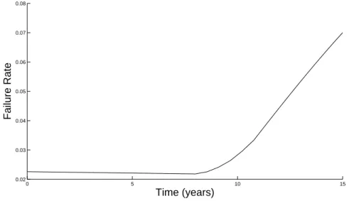
samples from the minimum information distribution for this example. It is given for machine 1, for the first 15 years of life, in Figure 6.
0 5 10 15
0.02 0.03 0.04 0.05 0.06 0.07 0.08
Time (years)
Failure Rate
Figure 6: The predictive distribution of the failure rate for machine 1 calculated using the 100 samples.
We see that the predictive distribution is smoother than the individual realisations from the simulation. In particular the changepoint between random failures and ageing is fairly smooth This is due to the averaging of the simulations in (6). We also see a slight non-linear quality to both sections of the failure rate in the predictive distribution. This is again as a result of averaging over non-linear quantities in (6).
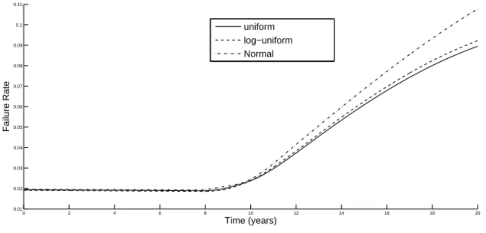
We can also use this example to examine the effect of the assumption of background distribution on the minimum information solution. In Figure 7 we see the predictive distribution for the failure rate of machine 1 under uniform, log-uniform and Normal background distributions for each of the parameters. All three choices of background distribution give a similar shape in the random failure period of the machine’s life. The uniform and log-uniform distributions also give very similar solutions in the ageing section of the plot. The predictive distribution using Normal background distributions is further from these in this section. This illustrates the way in which a sensitivity assessment can be made of the degree to which the distribution depends on assumptions made about the background distribution in the minimum information method. In this case it shows that the background distribution makes little difference except in the tail.
7. Example: Atmospheric dispersion and deposition
7.1. One-stage dispersion model
0 2 4 6 8 10 12 14 16 18 20 0.01
0.02 0.03 0.04 0.05 0.06 0.07 0.08 0.09 0.1 0.11
Time (years)
Failure Rate
uniform log−uniform Normal
Figure 7: The predictive distribution of the failure rate for machine 1 calculated using the 100 samples under uniform, log-uniform and Normal background distributions.
power plant. One commonly used model to describe such a process is the Gaussian plume model. This model is based on simplifying assumptions such as a constant wind direction, no plume rise and the land over which the contaminant is travelling being fairly even, [7].
The model is defined in terms of the downwind distance x from the source, the crosswind displacement y and the vertical displacement z. It then assumes that the plume concentration is of Gaussian form,
C(x, y, z) = Q0
2πuσy(x)σz(x)exp
− y 2
2σ2
y(x) exp
−(z−H) 2
2σ2
z(x)
+ exp
−(z+H) 2
2σ2
z(x)
,
whereC(x, y, z) is the time integrated concentration of the contaminant at (x, y, z),Q0
is the initial quantity of contaminant released,uis the windspeed andH is the centreline of the plume. The two standard deviations,σy(x) andσz(x), are the lateral and vertical plume spreads at x respectively. They are commonly assumed to follow deterministic power law models,
σy(x) = ayxby,
σz(x) = azxbz,
for unknown parameters ay, by, az, bz. That is, both lateral and vertical plume spreads are functions of the downwind distance.
Let us consider the lateral plume spread. The parameters of the power law model,
ay andby, do not have simple physical interpretations. They can be inferred from tracer experiments but this is unreliable. As they are unobservable we cannot elicit their values from experts. However,σyis observable. Having elicited a distribution forσywe can then use this to define probability distributions overay, by. This is probabilistic inversion.
concentration ratio,
C(x,0, H) = Q0 2πσyσzu
,
which is the Gaussian plume model evaluated aty= 0, z=H, is. Taking expectations and rearranging, if we elicit E[C(x,0, H)] from the expert, then
2πu Q0
E[C(x,0, H)] = E
1
ayazxby+bz
.
Since our notation is slightly different to that used up to now it is worth considering how this model fits into the framework we have adopted above. The model consists of three elements (C, σy, σz), so its outputs are the plume concentration and the lateral and vertical plume spreads. The model inputs areQ0,uandH. The model parameters
are (x, y, z), the place we are interested in plume concentration, which we choose, and
ay, by, az, bz which are unknown, and whose distributions will be inferred through PI.
7.1.1. Numerical illustration
Suppose we are interested in two downwind distances, 1km and 2km from the source. We could ask the expert for the expected lateral plume spreads and the concentration ratios at each of these distances. That is, the expert specifies,
E(σy,1) = E(ay) =α1, E(σy,2) = E(ay2by) =α2,
E
1
ayaz
=α3, E
1
ayaz2by+bz
=α4,
as described above for the plume spreads and ratios at 1km and 2km respectively. How-ever, the range of possible values forα2will depend on the chosenα1, the possible values
for α3 depend on α1 and α2 and so on. We shall find the minimum information
dis-tribution satisfying the constraints above using the methodology set out in Section 4. Some pseudo-code for defining a minimum information distribution in this way is given in Algorithm 2 in the Appendix.
The background distributions we use to find this minimum information distribution are taken to be uniform with respect to log(ay) log(az), by, bz. This follows work in Kraan and Bedford [2]. The discretizations take 50 points in each dimension with suitable ranges chosen for each parameter. The ranges used for the background distributions are
logay,logaz∈(0,4), by, bz∈(0,2).
Initially, given these ranges for the parameters, the possible ranges the expectations can take are
α1∈(1,55), α2∈(1,218),
α3∈(0,1), α4∈(0,1).
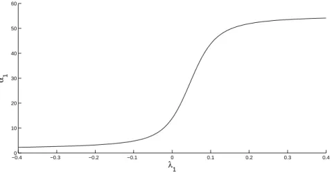
All are found by calculating the expectationαi for large positive and negative values of the relevantλi. Figure 8 indicates the range of possible values of the first constraintα1
and how they relate to the value ofλ1. We see that for large positive and negative λ1,
−0.40 −0.3 −0.2 −0.1 0 0.1 0.2 0.3 0.4 10
20 30 40 50 60
λ1 α 1
Figure 8: The possible range ofα1and corresponding values ofλ1.
We wish to find an initial value for α2 so we can calculate its range under this
specification for α1. Keeping λ1 = 0.116 and setting λ2 = 0 gives the expectations
α1= 45, α2= 97.691. Using this as a starting point we can calculate the range of values
α2 can take given thisα1. This is
α2|α1= 45∈(45,180).
We can see that some values which were possible originally are now not.
We can calculate the range of possible values forα2 given different specifications of
α1. Figure 9 shows these as points for 5 chosen values ofα1 and compares these to the
feasible region mapped out using the methods described in Section 5. We see that the two different methods are in agreement. The possible range of α2 is smallest for low
values ofα1 and larger for high values. It is always reduced from the original possible
range of (1,218).
Let us suppose that the expert, on receipt of this information, specifiesα2= 80. The
parameters of the minimum information distribution become
λ1= 0.1401, λ2=−0.0128.
Note thatλ1has changed asα1now depends on bothλ1 andλ2. Using these parameter
values andλ3= 0 leads to an initial expectation ofα3= 0.0082. From this we calculate
the range of possible values forα3. They are
α3|(α1= 45, α2= 80)∈(0.00336,0.186).
Again this is reduced from the original range.
If the expert specifiesα3= 0.0105 then the parameters of the minimum information
distribution areλ1 = 0.1425, λ2=−0.0128, λ3= 2.3025. Repeating this process for the
final constraint gives a feasible range of
0 10 20 30 40 50 60 0
50 100 150 200 250
α1
α2
Figure 9: The feasible region ofα2evaluated for different specified values ofα1.
This is significantly smaller than the initial possible range of (0,1). Therefore this process will be useful in guiding the expert to make a plausible choice forα4. If the expert settles
on α4 = 0.0038 then the final parameter values are λ1 = 0.1315, λ2 = −0.0124, λ3 = −0.4500, λ4= 4.8963.
7.2. Two-stage coupled dispersion and deposition model
Another quantity of interest when a contaminant is released into the atmosphere is how much of it is deposited into the ground at different distances from the source. This is known as deposition. Two different types are considered generally depending on the absence or presence of rain; dry and wet deposition.
Dry deposition can be measured in terms of the time integrated surface contamination at (x, y,0). This measures how much contaminant is deposited into the ground from the plume and is given by
Cd(x, y,0) = vdC(x, y,0),
= vd
Q0
πσyσz exp
−
y2
2σ2
y
+ H
2
2σ2
z
where vd is an unknown parameter called the dry deposition velocity. We can elicit expectations forCd(x, y,0) at different downwind distances and crosswind displacements. We see that the dispersion and deposition models are coupled.
In this two-stage example we shall consider eliciting expectations for the lateral plume spread and the surface contamination at the two downwind distances considered previ-ously and a crosswind displacement of 1km. That is, we elicit the means of
Thus, the first two constraints,α1andα2, are the same as in Section 7.1.1. We also have
α3 = E[Cd(1,1,0)],
α4 = E[Cd(2,1,0)].
We then wish to use these elicited values to define minimum information distributions over the model parameters
Ω = (ay, by, az, bz, vd).
Background distributions will be as previously foray, by, az, bz and uniform on the log-scale forvd as it is multiplicative.
7.2.1. Numerical Illustration
The first two expectations, α1 and α2, will have the same initial possible ranges as
previously. The corresponding initial ranges forα3andα4 are
α3 ∈ [1×10−4,0.1931],
α4 ∈ [1×10−4,0.1931].
We will setα1 = 45 and α2 = 80 as previously. However, first suppose that in order
to do so it is decided that no matter what the values of other constraints α2 must be
80. Therefore when we wish to specify α1, this specification for α2 defines an implicit
relationship forλ1, λ2. A plot of the curve representing this relationship is given in Figure
10.
−0.1 0 0.1 0.2 0.3 0.4 0.5 0.6
−0.03 −0.02 −0.01 0 0.01 0.02 0.03 0.04
λ1
λ2
Figure 10: The curve representing the the implicit relationship betweenλ1 and λ2 having specified
α2= 80.
As before this leads to parameter values of λ1= 0.1401 and λ2 =−0.0128. We now
This includes a new model parametervdas well as all of the dispersion model parameters from the one step example. It also includes the input from the dispersion model, x, as well as a new input,y.
We proceed as in the one step case. Initially we setλ3 = 0 to find a starting point
forα3 of 6×10⁻⁴. Working from this we find the range of possible specifications forα3
given the two constraints, which is
α3|(α1= 45, α2= 80)∈[1×10−4,3.9×10−3].
Suppose that, given this range, the expert specifies α3 = 6.5×10⁻⁴. The parameter
values which satisfy all three specifications areλ1 = 0.1207, λ2=−0.0121, λ3= 0.2459.
We proceed in the same manner for α4. Setting λ4 = 0 gives an initial value forα4 of
2×10⁻⁴. This allows us to calculate the admissible range forα
4given these specifications
for the other constraints. It is
α4|(α1= 45, α2= 80, α3= 6.5×10⁻⁴)∈[1×10−4,6×10−4].
Suppose we selectα4= 2.14×10⁻⁴. Then
λ1= 0.1207, λ2=−0.0121, λ3= 0.0403, λ4= 0.6758.
Thus we have fully defined the minimum information distribution which satisfies the four constraints for this two-stage example in such a way that ensures the expert always gives feasible values.
7.3. Discussion
Within the example we have worked with constraints sequentially, one at a time. In doing so it is clear that the order in which the expectations are specified is of importance. In some cases the order will be clear. For example, in a chain of models in which the output of one model is the input of the next, the constraints follow a natural order. However, this will not always be the case.
In a subjective expert elicitation procedure psychological anchoring occurs when an expert is given a value for an unknown (the anchor) and is then asked to adjust this in light of new information. The adjustment the expert makes has been found, Slovic [13], to be too small in general. Hence the expert is anchored by the original value, whether or not that value is accurate.
By sequentially specifying the expectation values in this minimum information ap-proach we are introducing another form of anchoring, which we shall refer to as quan-titative anchoring. That is, having specified the initial expectation, the expert is then anchored within the reduced range for the second expectation. They are then anchored to the new range for the third expectation given the first two, and so on. Clearly the order in which this takes place could have an effect on the resulting probability distribu-tions for the model parameters. More work is needed to investigate a suitable procedure for deciding on the order to specify the constraints in light of this anchoring.
8. Conclusion
In this paper we have investigated an approach to uncertainty modelling on coupled models in which an expert specifies the values of expectations of observable model outputs and these are used to specify probability distributions on unobservable model parameters. Generally this problem is either over- or under-specified and the methodology developed deals with both situations.
For under-specified problems we have solved for the distribution on the unobservable model parameters which has minimum information. This has been achieved numerically by first discretizing the problem. To avoid over-specification we consider a process of specifying the constraints sequentially. This is useful as it allows us to guide the expert in choosing values that do not conflict with previously chosen values.
The extension of this methodology to coupled models has allowed us to examine the range of possible values constraints can take for a second model, which can have some model inputs and outputs in common with the first model and others unique to itself. Again, the specifications of expectations for model outputs in the first model has an effect on the possible values of constraints in the second model.
The main advantage we see for this approach to modelling is that its flexibility enables us to build in features that we would qualitatively like to see, such as the onset of ageing in the second example or the physical models of the first example. The uncertainty modelling can then be carried out around these qualitative features. Rather than working with models which are mathematically convenient, we can work with models that possess the right qualitative properties.
The main difficulties of working with minimum information distributions are that they require numerical computation. While the curse of dimensionality is applicable here as in any other approach, there are opportunities to speed up numerical computation, for example by using variable grid sizes, and interesting opportunities to develop measures of coherence associated to the Lagrange multipliers.
Acknowledgements
The research in this paper was supported by EPSRC grant EP/E018084/1. The authors are grateful to two referees for comments and suggestions which improved the paper.
Algorithm 1Exploration in a radial direction of the feasible region of a 2 dimensional minimum information distribution.
Set radius tor
Define background distributions for x1, x2
fori←1, . . . , pdo
ei =hi(x1, x2)
end for
Define λ1 as a discretization on [−1,1]
λ(2p)=
p
1−λ2 1
λ(2n)=−
p
1−λ2 1
λ1=rλ1
λ(2p)=rλ(2p) λ(2n)=rλ
(n) 2
λi= (λ1,i, λ
(p) 2,i, λ
(n) 2,i)
fori←1, . . . ,length(λ1)do
α1,i= Eλi[h1(x1, x2)]
α2,i= Eλi[h2(x1, x2)]
end for
Algorithm 2 Defines the minimum information distribution satisfying (E[h1(x)], . . . ,E[hp(x)]) = (e1, . . . , ep).
Set background distributions forx1, . . . , xp
α1=e1
λ(1)1 = 0
fori←2, . . . , ndo
λ(1i)=λ (i−1) 1 −[ψ(λ
(i−1)
1 )−α1]/ψ ′
(λ(i−1)
1 )
end for
forj ←2, . . . , pdo
αj= (αj−1, ej)
λ(1)j = (λ
(n)
j−1,0)
fori←2, . . . , ndo
λ(ji)=λ
(i−1)
j −[ψ(λ
(i−1)
j )−αj]/ψ
′
(λ(i−1)
j )
Algorithm 3Simulation from a minimum information distributiong(x) of a sample of sizeN based on discretizationsxj,kof each variablexj.
fori←1, . . . , N do
(u1, . . . , up) sampled from independent uniform distributions on [0,1]
fork←1, . . . , m do
d1(x1) =g(x1)
D1(x1) =G(x1)
if D1(x1)> u1 then
˜
x1=x1,k
end if end for
forj←2, . . . , pdo fork←1, . . . , m do
dj(xj) =g(xj|˜x1, . . . ,x˜j−1)
Dj(xj) =G(xj|x˜1, . . . ,x˜j−1)
if Dj(xj,k)> uj then ˜
xj=xj,k Stop
end if end for end for end for
References
[1] T. Bedford and R. Cooke. Probabilistic Risk Analysis: Foundations and Methods. Cambridge
University Press, Cambridge, 2001.
[2] B. Kraan and T. Bedford. Probabilistic inversion of expert judgments in the quantification of model
uncertainty.Management Science, 51(6):995–1006, 2005.
[3] Dorota Kurowicka and Roger Cooke. Uncertainty Analysis - with High Dimensional Dependence
Modelling. Wiley, 2006.
[4] T.J. Bedford. Interactive expert assignment of minimally-informative copulae. In B. Lindqvist,
editor,Proceedings of Mathematical Methods in Reliability 2002. 2002.
[5] E. T. Jaynes.Probability Theory: the Logic of Science. Cambridge, 2003.
[6] J. Borwein and A. Lewis. Convex analysis and nonlinear potimization: theory and examples.
Canadian Mathematical Society, 2006.
[7] F.L. Harper, L. Goosens, R. Cooke, J. Helton, S. Hora, J. Jones, B. Kraan, C. Lui, M. McKay, L. Miller, J. Pasler-Sauer, and M. Young. Joint USNRC/CEC consequence uncertainty study: Summary of objectives, approach, application, and results for the dispersion and deposition uncer-tainty assessments. Technical report, NUREG/CR-6244 and EUR 15855 and SAND94-1453, Sandia National Laboratories and Delft University of Technology, Washington DC.
[8] O. E. Lanford. Entropy and equilibrium states in classical statistical mechanics. In A. Lenard,
editor,Statistical Mechanics & Mathematical Problems, volume 20 ofSpringer Lecture Notes in
Physics, pages 1–113. 1973.
[9] T. Bedford and K.J. Wilson. On the construction of minimum information bivariate copula families.
Submitted to Annals of the Institute of Statistical Mathematics, 2012.
[10] T. Bedford, A. Daneshkhah, and K.J. Wilson. Approximate uncertainty modeling with vine copulas.
Submitted to Operations Research, 2012.
[11] P.J. van Gestel. Kmoss, a maintenance optimization support system. InProc. Scand. SRE Symp.,
Studsvik, Sweden, 1990.
[13] P. Slovic. From shakespeare to simon: speculations - and some evidence - about man’s ability to