Contents lists available atSciVerse ScienceDirect
Computer-Aided Design
journal homepage:www.elsevier.com/locate/cad
Learning-based ship design optimization approach
Hao Cui
∗, Osman Turan, Philip Sayer
Department of Naval Architecture and Marine Engineering, University of Strathclyde, Glasgow, G4 0LZ, United Kingdom
a r t i c l e i n f o
Keywords: Machine learning Ship design
Structure optimization Structure analysis Multi-objective optimization
a b s t r a c t
With the development of computer applications in ship design, optimization, as a powerful approach, has been widely used in the design and analysis process. However, the running time, which often varies from several weeks to months in the current computing environment, has been a bottleneck problem for optimization applications, particularly in the structural design of ships. To speed up the optimization process and adjust the complex design environment, ship designers usually rely on their personal experience to assist the design work. However, traditional experience, which largely depends on the designer’s personal skills, often makes the design quality very sensitive to the experience and decreases the robustness of the final design. This paper proposes a new machine-learning-based ship design optimization approach, which uses machine learning as an effective tool to give direction to optimization and improves the adaptability of optimization to the dynamic design environment. The natural human learning process is introduced into the optimization procedure to improve the efficiency of the algorithm. Q-learning, as an approach of reinforcement learning, is utilized to realize the learning function in the optimization process. The objective particle swarm optimization method, multi-agent system, and CAE software are used to build an integrated optimization system. A bulk carrier structural design optimization was performed as a case study to evaluate the suitability of this method for real-world application.
©2011 Elsevier Ltd. All rights reserved.
1. Introduction
Ship design is a complex and distributed process, and with the development of computer applications in ship design, optimization plays an important role in this process. Optimization has been a particularly effective tool in ship structural design and analysis; however, the length of time required for optimization, which often lasts from weeks to months, has been a bottleneck problem for practical applications. Designers always try to reduce the runtime and speed up the convergence of optimization as much as possible. One of the most common methods is to use the designer’s experience to assist the optimization. However, the specialist’s experience and skills depend too much on personal ability, which means that the design process will become very sensitive and the design quality cannot be guaranteed. At the same time, the design conditions and variables often change dynamically during the whole design process, thus making the design very unstable.
This paper presents a new machine-learning-based optimal ship design approach, which introduces the human learning process into the practical ship design and analysis to improve the efficiency of optimization. Reinforcement learning as an important machine learning method is employed here to solve the sensory
∗Corresponding author. Tel.: +44 01415484890; fax: +44 01415522879.
E-mail address:[email protected](H. Cui).
memory and partial short time memory problem due to its satisfactory real-time learning performance. Q-learning, as an idiographic approach of reinforcement learning, is selected and realized via a multi-agent system in this study. This method can guide the direction of optimization via experience learning and can assist the system to further adjust the ship design environment. The proposed method is tested on a real bulk carrier structural design case. The paper begins with an introduction of the work, followed by the background of optimization applications in ship design and structural analysis. Section3presents the new learning-based ship optimization method together with a brief introduction of human learning theory. Section 4focuses on the application of the proposed approach on ship structural design, while the advantages and disadvantages of the application of this method are discussed in Section5.
2. Background
Due to the complexity and dynamics of ship design, naval architects try to use many types of reliable and adaptive approaches to assist in the design work geared at improving the design quality. With the development of CAD and CAE technology in computer science, optimization has become more and more important, both in improving the performance of vessels and in obtaining better economic benefits while satisfying the requirements of rules and regulations. During the 1960s, the
concept of computer-aided ship design began to appear, enabling the computer to play a more important role in ship design [1]. With the rapid popularization and development of computer-aided ship design, this has become an important research direction of ship design. These optimization methods are powerful tools that greatly reduce the complexity of design work and improve the quality of the final solution. As per the available research results, the MOGA (multi-objective genetic algorithm) – one type of heuristics method – appears to be a promising solution to complex ship design optimization problems.
[image:2.595.308.548.58.215.2]Ray and Sha [2] incorporated accepted naval architectural es-timation methods, a decision system handler, a nonlinear opti-mization tool and a containership model for the application. Ray et al., in [3–5], also provided a partial discrete optimization model, a global optimization model and an artificial neural network (ANN) application for ship design, respectively. A back propagation net-work model that undergoes supervised training was accepted, and the structure of the neural nets with the method of implementa-tion was given. Thomas [6,7] used Pareto ranking, MOGA and NPGA to investigate the feasibility of full-stern submarines. Three objec-tives were considered: maximization of the internal volume, mini-mization of the power coefficient for ducted propulsor submarines, and minimization of the cavitation index. Binary representation and different selection techniques were used. Thomas also com-pared several different algorithms and reached the conclusion that MOGA outperforms the other methods in all of the aspects con-sidered. Brown and Thomas [8] used a GA with Pareto ranking for naval ship concept design. Two objectives were considered: maximization of the overall measure of effectiveness (this factor represents customer requirements and relates ship measures of performance to mission effectiveness) and minimization of life-cycle cost. A binary representation and roulette wheel selec-tion with stochastic universal sampling were used. Brown and Salcedo [9] and Brown and Mierzwicki [10]introduced a multi-objective genetic algorithm in naval ship design. Todd and Sen [11] used a variant of MOGA for the pre-planning of containership lay-outs (a large-scale combinatorial problem). Four objectives were considered: maximization of the proximity of containers, mini-mization of the transverse center of gravity, minimini-mization of the vertical center of gravity, and minimization of unloading. A binary representation and roulette wheel selection with elitism based on non-dominance were used. They used the same algorithm for the cutting shop problem in the shipyard [12,13]. Two objectives were considered: minimization of the makespan and minimization of total penalty costs. Ray et al. [14] presented an evolutionary al-gorithm for generic multi-objective design optimization problems. This algorithm was based on nondominance of solutions in the ob-jective space and constraint space and used effective mating strate-gies to improve solutions that were weak in either spaces. Ray and Tsai [15] applied a swarm algorithm for the shape optimization of airfoils on single- and multi-objective optimization. The proposed swarm algorithm was based on a socio-behavioral model, and three different airfoil designs were used as case studies. Peri and Campana [16] proposed a multidisciplinary design optimization of a naval surface combatant and developed high-fidelity models and multi-objective global optimization algorithms in simulation-based design [17]. Ölçer [18] proposed a hybrid approach for multi-objective optimization problems in ship design and shipping. In his study, the software ‘modeFRONTIER’ was used to perform the optimization via MOGA. Boulougouris and Papanikolaou [19] in-troduced a multi-objective optimization of a floating LNG termi-nal and utilized the software ‘modeFRONTIER’ with MOGA. Pinto et al. [20] presented a deterministic method for multi-PSO and ap-plied the method to the multi-objective (two objectives) seakeep-ing of the containership problem. Cui and Turan [21] proposed a new multi-PSO method, HCPSO, and applied it to three objective optimization of ship stability design.
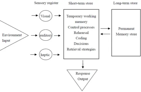
Fig. 1. The model of Atkinson and Shiffrin summarized by Baddeley.
Rigo [22] published a detailed, state-of-the-art paper in 2003 on a structural optimization research field. He introduced the concept and development of ship structure optimization from the 1960s to 2003. In the same paper, Rigo introduced the optimization software LBR-5, while Richir et al. [23] used this software [22] to solve a three-objective optimization problem. The production cost, weight and moment of inertia were selected as objectives, and a two-stage local search heuristic approach (CONLIN) was accepted as the optimization algorithm. Zanic et al. [24] introduced a decision support methodology including optimization for a multi-deck ship structure. Klanac [25] proposed vectorization and constraint-grouping approaches to enhance the optimization of a fast ferry structure. Klanac [26] introduced a two-stage optimization approach for collision simulation. Eamon and Rais-Rohani [27] presented a reliability-based optimization method for a composite advanced submarine sail structure. Jang [28] employed a multi-objective genetic algorithm to solve a two-objective optimization problem. Sekulski [29] used a genetic algorithm to solve the problem of weight minimization of a high-speed vehicle–passenger catamaran structure.
3. Learning-based ship optimal design method
The learning-based ship optimal design method aims to simulate natural human learning to assist ship optimization design. Therefore, the design system can draw experience from design actions automatically to assist the ongoing work. In this method, the ship design process can be analogized to the life of a human. During every single design process, the method will learn the instantaneous experience, and following a particular design exercise, this experience may be valued as very useful knowledge to store in the system. With the increasing number of the design cases, the system will improve its ability step by step via learning.
3.1. Brief introduction of learning theory
Although learning science has been developed since the 1990s [30], the mechanism of human memory storage is very complex, and the detailed process of memory storage has been a vexing subject of research for a long time. In this study, the popular learning model of Atkinson and Shiffrin was accepted along with the improved working memory concept developed by Baddeley [31].
In the memory model of Atkinson and Shiffrin (as shown in
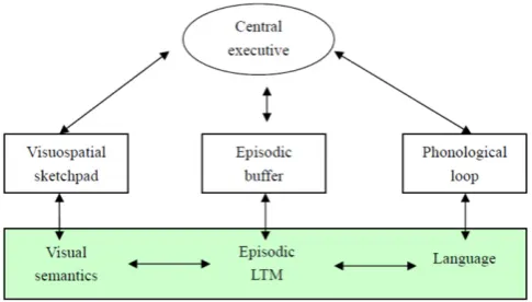
Fig. 2. Multi-component working memory model of Baddeley.
to remember the rules of things. Short-term memory is the most important part of the entire memory process. It selects appropriate sections in the sensory memory to transfer to the long-term memory and will abandon other sections. However, as the most complex part in learning theory, memory is still a subject of debate. In this study, the working memory theory used to describe short-term memory is accepted.
Fig. 2explains the working memory model of Baddeley [32]. Memory is processed by a central executive. Multiple components, which include a visuospatial sketchpad, episodic buffer and phonological loop, activate the central executive to help in remembering. Thus, the working memory functions via many types of perception methods.
3.2. The multi-objective optimization
A general multi-objective optimization problem (also called multiple criteria optimization, multi-performance or vector opti-mization) is to find the design variables that optimize a vector ob-jective function (F
(
Y)
= {
f1(
Y),
f2(
Y), . . . ,
ft(
Y)
}
) over a feasibledesign space. The objective functions are the quantities that the de-signer wishes to minimize, maximize, or attain at a certain value. This problem can be formulated as follows:
Minimize
:
F(
Y)
= {
f1(
Y),
f2(
Y), . . . ,
ft(
Y)
}
Subject to
:
pinequality constraintsgδ(y
)
≥
0, δ
=
1, . . . ,
pqequality constraintshΦ
(
y)
=
0,
Φ=
1, . . . ,
qwhereY
= [
y1,
y2, . . . ,
yn]
is the vector of decision variables.In multi-objective optimization, the objectives are usually in conflict with each other. The aim of multi-objective optimization is to find a solution that is acceptable to decision makers.
Design variables are the numerical quantities for which values are to be chosen in an optimization problem. In most engineering applications, the design variable is controllable by designers according to factual problems. Design variables usually have maximum and minimum boundaries that can be treated as separate constraints.
There are various restrictions from the environment or resources (e.g., physical limitations, time restrictions, etc.) that must be satisfied to develop an acceptable solution in an optimization problem. These restrictions are generally called constraints and may be explicit or implicit.
In multi-objective optimization, the aim is not just to find a sin-gle solution as a global optimization but to find good compromises (or ‘‘trade-offs’’). Here, Pareto optimality is introduced. For a multi-objective optimization problem, any two solutionsy1andy2can have one of two possibilities: one dominates the other or neither dominates. In a minimization problem, without loss of generality,
a solutiony1dominatesy2if the following two conditions are sat-isfied:
∀
γ
∈ {
1,
2, . . . ,
t} :
fγ(
y1)
≤
fγ(
y2)
∃
λ
∈ {
1,
2, . . . ,
t} :
fλ(
y1) <
fλ(
y2).
(1)If any of the above conditions are violated, the solutiony1does not dominate the solutiony2. Ify1dominates the solutiony2,y1 is called the dominated solution. The solutions that are non-dominated within the entire search space are denoted as Pareto-optimal and constitute the Pareto-Pareto-optimal set or Pareto-Pareto-optimal frontier.
3.3. Learning-based ship optimal design
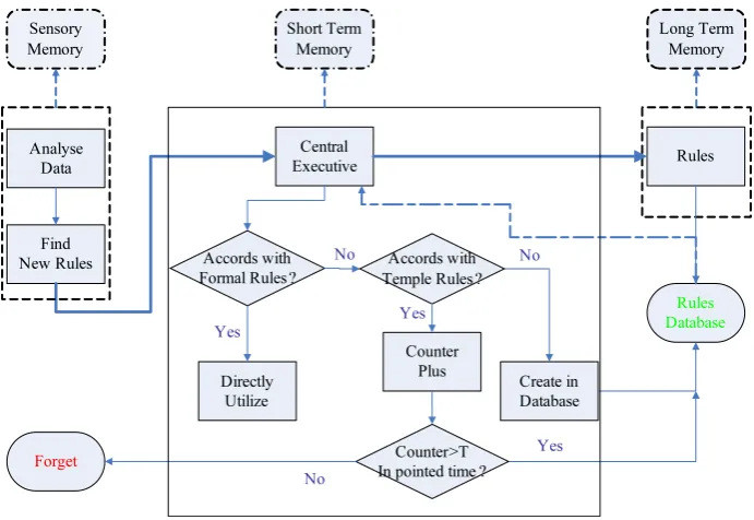
Schank [33] studied dynamic learning and pointed out that to build an expert system, two possible avenues are open. One is to attempt to obtain compiled knowledge of the expert. The other is to attempt to model the raw memory of the expert. This study accepts the latter viewpoint. The entire process of ship design optimization can be divided into three parts according to memory theory. Every part simulates a relevant learning function as shown inFig. 3.
The sensory memory portion, defined by psychologists as immediate memory, is used here to search for new experiences in the optimization process, which are learned by trial and error. For every design process, the design task may be different, and the experience gained from each run may not be suitable for other designs. First, the proposed method should analyze the data and distinguish to what type of design task it belongs. Furthermore, the method should attempt as much as possible to draw rules/relations from data. These rules can be selected for long-term memory in the future and may be abandoned.
Short-term memory, under the working memory theory, is the most important part of this method. This part is managed via a ‘‘central executive’’ center. The central executive first checks the new rule in the database to determine whether it has already been a formal rule. A formal rule here indicates a rule that comes from mature or reliable knowledge, such as classification society rules, regulations of IMO, etc. Formal rules also include the rules that are used in previous designs and which have been proven as reasonable and available recourses. If the new rule is a formal rule that has been stored in the system, it can be directly used. If not, the central executive will continue to check whether the new rule belongs to temple rules. Temple rules indicate rules that have been proven correct at least twice in past design work. Every temple rule has a counter. If the new rule belongs to the temple rules, then the counter of this temple rule will add a value of one. If not, the method will create a new rule and allocate the relative counter, which is zero in this case. The counter in this part is used to check the availability of the rules. The central executive also checks the counter of every temple rule after a predefined time. If the counter exceeds a given value, the central executive will change this temple rule to a formal rule. If the counter cannot match the given value, a time-checking index will be given to this counter. After three iterations of continuous predefined time checking, if the counter of the temple rule still cannot satisfy the given requirement, this temple rule will be removed from the database.
The long-term memory, presented by Baddeley, is used to store information for a sufficiently long time to be accessible over any period lasting more than a few seconds. InFig. 3, the ‘‘long-term memory’’ indicates the rules and regulations system that has been proven to be correct and effective.
Fig. 3. A single run of machine-learning-based ship optimal design.
Fig. 4. Classic reinforcement learning model.
environment. Reinforcement learning can be handled well in real-time learning. In a classic reinforcement learning model, an agent is connected to the environment via perception and action. In the model shown inFig. 4,Bis an agent andT is the environment.
In the first step, agentBreceives an input ‘i’; in the second step, agentBchooses an action ‘a’ to generate an output. This action ‘a’ changes the environmentT, and in the third step, the value of this state transition is communicated to agentBthrough a scalar reinforcement signal, ‘r’. The agent’s behavior,B, should choose actions that tend to increase the long-run sum of the values of the reinforcement signal. It can learn to do this over time by systematic trial and error, guided by a wide variety of algorithms.
Q-learning, an excellent approach to implement real-time learning, is selected in this method to assist the algorithm used to find hidden rules.Q-learning ([34, # 30] and [35]) operates by learning an action-value function that gives the expected util-ity of taking a given action in a given state and following a fixed policy thereafter. As a form of model-free reinforcement learning, which means Q-learning can compare the expected utility of the available actions without requiring a special envi-ronment, the requirement ofQ-learning is flexible with respect to the type of environment. However, this does not mean that
Q-learning is applicable for all situations. Compared to a contin-uous environment, a discrete environment is more suitable for the current development ofQ-learning. Meanwhile, the discrete and finite engineering environment is one important characteristic of
ship design optimization. The combination ofQ-learning and ship design optimization is therefore reasonable.
ForQ-learning, a deterministic Markov decision process (MDP) is one in which state transitions are deterministic. In a nonde-terministic MDP, a probability distribution function defines a set of potential successor states for a given action in a given state. If the MDP is non-deterministic, the iteration of values requires that we determine the action that returns the maximum expected value. Theoretically, value iteration is possible in the context of nondeterministic MDPs. However, in practice, it is computation-ally impossible to find the necessary integrals without additional knowledge or some modification.Q-learning solves the problem by taking the maximum value over a set of integrals. Rather than finding a mapping from states to state values (as in value itera-tion),Q-learning finds a mapping from state/action pairs to values (calledQ-values). Instead of having an associated value function,
Q-learning makes use of theQ-function. In each state, there is a
Q-value associated with each action. The definition of aQ-value is the sum of the (possibly discounted) reinforcements received when performing the associated action and then following the given policy thereafter. Likewise, the definition of an optimal
Q-value is the sum of the reinforcements received when perform-ing the associated action and then followperform-ing the optimal policy thereafter. Eq.(2)is a general expression.
Q
(
xt,
ut)
=
r(
xt,
ut)
+
γ
max ut+1Q
(
xt+1,
ut+1).
(2)From Eq. (2), Q-learning differs from other value iteration reinforcement learning in that it displays the relationship of given actions and expected values of the successor states. It does not require that in a given state, each action be performed and the expected values of the successor states calculated.
The learning process seeks solutions to Eq.(2). Before learning begins,Q-learning returns a fixed value chosen by the designer. Then, each time, the agent is given a reward (the state has changed). New values are calculated for each combination of state
sfromS, which are statement sets and action a fromA, which are action sets. It assumes the old value and makes a correction based on the new information as shown in Eq.(3).
Q
(
st,
at)
←
Q(
st,
at)
+
η
× [
rt+1 [image:4.595.54.265.325.449.2]Fig. 5. Offspring reproduction using a genetic algorithm.
wherertis the reward given at timet
, η (
0< η
≤
1)
is the learningrate, which may be the same value for all pairs. The discount factor
γ
is 0≤
γ <
1. Eq.(3)is equivalent toQ
(
st,
at)
←
Q(
st,
at)(
1−
η)
+
η
[rt+1+
γ
maxQ(
st+1,
at+1)
].
(4)Eq.(4)is the formula used in this study.
NSGAII (Non-dominated sorting genetic algorithm-II) was pro-posed by Baddeley [31] as a fast and elite multi-objective algo-rithm. This algorithm uses the crowding distance parameter to maintain diversity in the population and defines the constraint-dominance principle to function better with constrained optimiza-tion problems.
NSGAII can be divided into three main parts: non-dominated sorting, crowding distance assignment, and offspring selection with respect to fitness and crowding distance. In the sorting procedure, non-dominated individuals are found in the population through Pareto-dominance principle and assigned a rank zero; then, the algorithm begins to seek the next front and so on. The crowding distance assignment is used to penalize individuals that are close to each other.
In NSGAII, the parent and child populations are combined together to select the next offspring using roulette wheel selection and the selection method of the GA. The proposed method employsQ-learning to improve the selection of offspring. Through the offspring reproduction mode of NSGAII, the crossover and mutation operations, which are often used in genetic algorithms, are employed in NSGAII to generate the next-generation population.
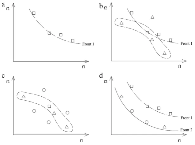
Fig. 5shows a common method of producing offspring using a genetic algorithm. Assume that there are four solutions in the processing of a genetic algorithm, which belong to the same front, as indicated inFig. 5(a) by squares. Now, the task is to produce the next-generation solutions via these four solutions. InFig. 5(b), four children (represented by triangle) are obtained via crossover and mutation operations. Then, the parent (square) and children (triangle) are collected together for sorting, and four of them, which lie within the dashed circle, are selected as new parents, which are defined as the second-generation parents. Then, these four parents are processed via crossover and mutation operations, again to breed new children defined as the second-generation
children. As shown in Fig. 5(c), there are eight solutions now including the four second-generation parents and four children. The algorithm will select four of these eight solutions using a particular selection method to form Front 2 shown inFig. 5(d). Then, the algorithm will iterate this process until it finds the final Pareto-optimal solutions.
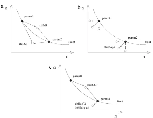
Fig. 6displays the offspring process of a new hybrid algorithm. InFig. 6(a), the offspring are the same four initial points, though an index ofQ-learning, such asIp1−1, is given to these points, which is the index of the parent in the first front; the serial number of this parent is ‘‘1’’. In the initial stage, all indexes are set to 0. Then, four children are produced according to the same GA method, which will also be provided indexes and assigned zero for the index value. At this stage, the parents and children, eight in total, are combined together for comparison in selecting the next generation of parents, which will be used to breed the next generation children. This process in the new hybrid algorithm still accepts the same fitness-based method as that inFig. 5, and in the following step, four candidates from these eight solutions are selected as the second-generation parents; their indexes are set to 1, while those of others are assigned a value
−
1 as shown inFig. 6(b).Fig. 6(c) shows the new second-generation children production process. Compared to Fig. 5(c), the whole area of reproducing children is closer to the range of indexes equaling 1. This is only a schematic diagram; the real operation is processed viaQ-learning.Fig. 6(d) shows the final front of the new hybrid method.Fig. 7 illustrates the detailed offspring generation process in the new hybrid algorithm. The parents are also randomly selected from the parent group. The crossover and mutation operations are processed as other evolutionary algorithms, but this time, only one child is selected as offspring from child1 and child2, as shown in Fig. 7(a). Here we assume that child1 is selected and child2 will be recalculated from the Q-learning approach. The hybrid algorithm will calculate theQ-value in the pointed ranges around parent1 and parent2, and it will then be compared to all calculated
Q-values. The child who has the greatestQ-value child-q-a (in
Fig. 7(b)) will be selected as child-f-2 in the next generation in
Fig. 6. Offspring reproduction in new hybrid algorithm.
Fig. 7. Detailed method of producing offspring in new hybrid algorithm.
4. Case study
Ship structural optimization is an important part of ship design. Like other optimization problems in this field, the time cost has a great influence on structural optimization. For a merchant ship under the current computing environment, ship structural optimization usually lasts several weeks or months.
In this case study, the structural optimization of the midship section of a bulk carrier is carried out. This is a 50,000 DWT handymax bulk carrier (shown inFig. 9), the main dimensions of which are provided asTable 1.
The objectives of this practical optimization focus on the structural weight control and fatigue coefficient. The optimization constraints are set according to common structural rules (CSRs) of the International Association of Classification Societies (ICAS, Consolidated Effective as of 1 July 2009 # 33); the stress and fatigue are also evaluated according to the CSR methods. The first
Table 1
Main dimensions of bulk carrier in case study.
Length (m) 190
Breadth (m) 32.2
Depth (m) 17.5
Design draft (m) 11.2
Scantling draft (m) 12.8
Cargo capacity (m3) 68 000
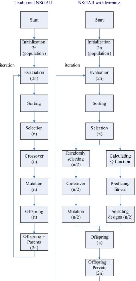
[image:6.595.137.451.304.547.2] [image:6.595.306.553.597.653.2]Fig. 8. The traditional NSGAII and learning-based NSGAII.
a refined mesh in this case. The cumulative fatigue damage D
calculated for the combined equivalent stress should comply with the following criteria:
D
=
j
Dj
≤
1.
0where Dj is the elementary fatigue damage for each loading
condition ‘‘j’’.
The loads in this case study are selected according to the CSR of the IACS and the original design data. If the original design data provide the detailed values of the loads and, at the same time, these values are greater than the values calculated from the CSR, then the original design values will be used; otherwise, the values will be calculated according to the CSR. In certain calculations, values in the design proposal will be used to define the still-water bending moments.
MSW,H
=
MSW,H(
design)
=
1 700 000 kN mMSW,S
=
MSW,S(
design)
=
1 500 000 kN m.
The still-water shear force is also provided by the design proposal:
QSW
(
±
)
=
8.
5920×
104kN.
Other loadings are calculated according to the CSRs. In this case study, the loading case is added via ABAQUS with FORTRAN to assist in simulating loadings. The inertial pressure due to the liquid is not considered in the current situation.
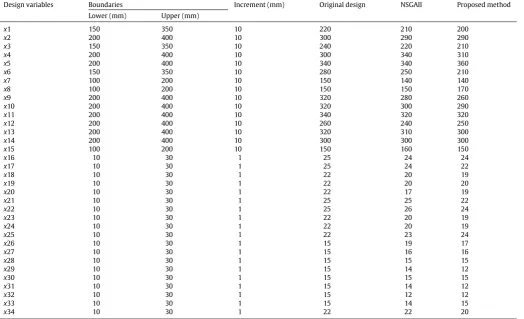
There are 34 design variables (as shown inFig. 10). The design variables fromx1 tox15 are the size of the longitudinal stiffeners and from x16 to x34 are the shell thicknesses in mm. Table 2
lists the minimum and maximum of the design variables together with the changing increments. The upper bound of the longitudinal stiffener is 400 mm, and the lower bound is 100 mm. The increment is 20 mm. The upper bound of the shell thickness is 10 mm, and the lower bound is 30 mm. The increment is 1 mm. The calculation was processed via JAVA coding and ABAQUS. The CAE model was built in ABAQUS (as shown inFig. 11). The parameters of NSGAII are shown inTable 3.
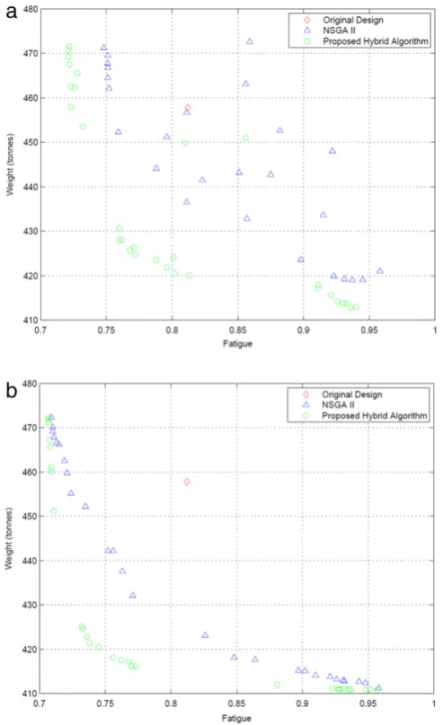
The optimizations were performed in the same computer environment and run four times for both the NSGAII and proposed algorithm. At the end of these four runs, a random sampling method was employed to compare the different algorithms. Here, the results from the third run of both algorithms were selected. Using the proposed method, 3000 different designs were obtained in the design space, with 569 of them being unfeasible designs. Therefore, 2431
(
=
3000−
569)
feasible designs were filtered in the design space to obtain only those designs that belonged to the Pareto front. For NSGAII, 2398 feasible designs were obtained. The selected solutions of the proposed method and NSGAII are listed [image:7.595.122.481.578.743.2]Fig. 10. Design variables of midship structure.
Table 2
Optimization variables with their types, bounds and results.
Design variables Boundaries Increment (mm) Original design NSGAII Proposed method Lower (mm) Upper (mm)
x1 150 350 10 220 210 200
x2 200 400 10 300 290 290
x3 150 350 10 240 220 210
x4 200 400 10 300 340 310
x5 200 400 10 340 340 360
x6 150 350 10 280 250 210
x7 100 200 10 150 140 140
x8 100 200 10 150 150 170
x9 200 400 10 320 280 260
x10 200 400 10 320 300 290
x11 200 400 10 340 320 320
x12 200 400 10 260 240 250
x13 200 400 10 320 310 300
x14 200 400 10 300 300 300
x15 100 200 10 150 160 150
x16 10 30 1 25 24 24
x17 10 30 1 25 24 22
x18 10 30 1 22 20 19
x19 10 30 1 22 20 20
x20 10 30 1 22 17 19
x21 10 30 1 25 25 22
x22 10 30 1 25 26 24
x23 10 30 1 22 20 19
x24 10 30 1 22 20 19
x25 10 30 1 22 23 24
x26 10 30 1 15 19 17
x27 10 30 1 15 16 16
x28 10 30 1 15 15 15
x29 10 30 1 15 14 12
x30 10 30 1 15 15 15
x31 10 30 1 15 14 12
x32 10 30 1 15 12 12
x33 10 30 1 15 14 15
x34 10 30 1 22 22 20
inTable 2 together with the original design; the final objective results are shown inTable 4. The results show that the weight of the structure was reduced significantly, while the fatigue performance of the structure improved at the same time.Table 4shows the half-weight of the whole block and the values in the brackets as the total weights. Due to the symmetry of the ship along the centerline, computation was carried out for only half of the ship. The weight of the whole block was reduced from 915.6 tonnes (original design)
Table 3
Parameters setting in case study for NSGAII.
NSGAII parameters setting
Parameters name Parameters value
SBX (Simulated binary crossover) 10
polynomial mutation 20
crossover probabilities 0.9
mutation probabilities 0.1
Population 30
Generation 100
Table 4
Results of optimization.
Original design
NSGAII Proposed method
Objective 1: weight(t) 457.8 (915.6) 432.1 (864.2) 420.5 (841) Objective 2: fatigue 0.812 0.771 0.745
Fig. 11. CAE model of midship structure.
In comparing the optimal solutions with the original solutions, it can be seen that the structures of the fatigue hot-spot area are evidently strengthened as other structures are reduced. Thus, when the weight of the whole structure is lightened, the fatigue damage index also decreases due to the enhancement in the local structure. In the future, more hot spots should be added to verify this phenomenon.
More importantly, for real design applications, compared to NSGAII, the proposed method converges faster and reduces computation and hence the design time significantly. In ship design, most of the computational time is not consumed in the optimization approach but rather through naval architectural calculations using third-party software. It is important to note that it sometimes takes hours for one fitness calculation. In this study, the solution began converging after the 64th generation in the proposed method, while the NSGAII began converging after the 82th generation (seeFig. 12). This means that the proposed method takes 25% less time in looking for Pareto solutions compared to NSGAII. In a more complex environment, such as that experienced by a real ship, this provides an advantage in terms of completing the design more quickly and thus at a lower cost. In the future, more tests will be conducted to compare the results with those of different algorithms. At the same time, the running times should also be improved.
5. Conclusions
This paper introduces a learning-based ship optimal design method. As an effective tool, machine learning is integrated into general optimization methods to improve the searching ability. Using this method, the process can assist new design development and provide significant time savings.
A real ship design case, the structural optimization of a bulk carrier with two conflicting objectives (weight and fatigue), was carried out. For the operation platform, a JAVA-based optimization system and ABAQUS were integrated into the optimization framework.
Fig. 12. Optimization solutions for case study: (a) the solutions obtained in the 64th iteration, and (b) the solutions obtained in the final iteration.
The proposed algorithm provides an improved design with respect to the original design for every chosen objective by a significant margin and demonstrates the value of this method. In this design case, the proposed algorithm displays better performance in terms of both speed and final results. The proposed algorithm is structured via a multi-agent system, and every agent works remarkably well. It can be concluded that the proposed approach shows great potential and can be applied to similar and even more complex optimization problems in ship design, as well as to related areas within the maritime industry.
References
[1] Nowacki H. Five decades of computer-aided ship design. Computer-Aided Design 2010;42:956–69.
[2] Ray T, Sha OP. Multicriteria optimization model for a containership design. Marine Technology 1994;31:258–68.
[3] Ray T, Gokarn RP, Sha OP. A partial discrete optimization model for preliminary ship design. Journal of Institution of Naval Architects 1994.
[4] Ray T, Gokarn RP, Sha OP. A global optimization model for ship design. Computers in Industry 1995;26:175–92.
[5] Ray T, Gokarn RP, Sha OP. Neural network applications in naval architecture and marine engineering. Artificial Intelligence in Engineering 1996;1:213–26. [6] Thomas M. A Pareto frontier for full stern submarines via genetic algo-rithm. Cambridge (Massachusetts, USA): Ocean Engineering Department, Mas-sachusetts Institute of Technology; 1998.
[image:9.595.44.295.79.161.2][8] Brown A, Thomas M. Reengineering the naval ship design process. In: Proceedings of from research to reality in ship systems engineering symposium. University of Essex. 1998.
[9] Brown A, Salcedo J. Multiple-objective optimisation in naval ship design. Naval Engineers Journal 2003;115:49–61.
[10] Brown A, Mierzwicki T. Risk metric for multi-objective design of naval ships. Naval Engineers Journal 2004;116:55–72.
[11] Todd D, Sen P. A multiple criteria genetic algorithm for containership loading. In: Proceedings of the seventh international conference on genetic algorithms. 1997. p. 674–81.
[12] Todd D, Sen P. Multiple criteria scheduling using genetic algorithms in a shipyard environment. In: Proceedings of the 9th international conference on computer applications in shipbuilding. 1997.
[13] Todd D, Sen P. Tackling complex job shop problems using operation based scheduling. In: The integration of evolutionary and adaptive computing technologies with product/system design and realisation. 1998.
[14] Ray T, Kang T, Seow KC. Multi-objective design optimization by an evolutionary algorithm. Engineering Optimization 2001;33:399–424. [15] Ray T, Tsai HM. A swarm algorithm for single and multi-objective airfoil design
optimization. AIAA Journal 2004;42:366–73.
[16] Peri D, Campana E. Multidisciplinary design optimisation of a naval surface combatant. Journal of Ship Research 2003;47:1–12.
[17] Peri D, Campana E. High-fidelity models and multiobjective global optimisa-tion algorithms in simulaoptimisa-tion-based design. Journal of Ship Research 2005;49: 159–75.
[18] Ölçer A. A hybrid approach for multi-objective combinatorial optimisation problems in ship design and shipping. Computers & Operations Research 2008; 35:2760–75.
[19] Boulougouris E, Papanikolaou A. Multi-objective optimisation of a float LNG terminal. Ocean Engineering 2008;35:787–811.
[20] Pinto A, Peri D, Campana E. Multiobjective optimisation of a containership using deterministic particle swarm optimisation. Journal of Ship Research 2007;51:217–28.
[21] Cui H, Turan O. Application of a new multi-agent based particle swarm optimisation methodology in ship design. Computer-Aided Design 2010;42: 1013–27.
[22] Rigo P. An integrated software for scantling optimization and least production cost. Ship Technology Research 2003;50:135–40.
[23] Richir T, Caprace JD, Lossseau N, Bay M, Parsons MG, Patay S, Rigo P. Multicriterion scantling optimization of the midship section of a passenger vessel considering IACS requirements. In: 10th international symposium on practical design of ships and other floating structure. 2007.
[24] Zanic V, Andric J, Prebeg P. Decision support methodology for concept design of multi-deck ship structures. In: 10th international symposium on practical design of ships and other floating structure. 2007.
[25] Klanac A, Jelovica J. Vectorization and constraint grouping to enhance optimization of marine structures. Marine Structures 2009;22:225–45. [26] Klanac A, Ehlers S, Jelovica J. Optimization of crashworthy marine structures.
Marine Structures 2009;22:670–90.
[27] Eamon CD, Rais-Rohani M. Integrated reliability and sizing optimization of a large composite structure. Marine Structures 2009;22:315–34.
[28] Jang B, Ko D, Suh Y, Yang Y. Adaptive approximation in multi-objective optimization for full stochastic fatigue design problem. Marine Structures 2009;22:610–32.
[29] Sekulski Z. Least-weight topology and size optimization of high speed vehicle-passenger catamaran structure by genetic algorithm. Marine Structures 2009; 691–711.
[30] Sawyer RK. The Cambridge handbook of the learning sciences. Cambridge University Press; 2006.
[31] Baddeley AD. Working memory. Oxford University Press; 1986.
[32] Baddeley AD. The episodic buffer: a new component of working memory? Trends in Cognitive Sciences 2000;4:417–23.
[33] Schank CR. Dynamic memory revisited. Cambridge University Press; 1999. [34] Watkins C. Learning from delayed rewards. University of Cambridge.
1989.