An intelligent and modular adaptive control scheme for automating the milling process

An intelligent and modular adaptive control scheme for

automating the milling process

Luis Rubio

*

, Andrew Longstaff, Simon Fletcher and Alan Myers

Centre for Precision Technologies, University of Huddersfield, UK

*[email protected]

ABSTRACT

This research work describes an intelligent and modular architecture for controlling the milling process. For this purpose, it is taking into account the admissible input cutting parameters given by the stability lobes and restrictions of the system, calculating the quasi-optimal cutting parameters. The quasi-optimal cutting parameters are obtained considering a cost function with multi-objective purpose. Furthermore, parallel multi-estimation adaptive control architecture is proposed in order to allow adaptation of the system when the cutting parameters are changed, for example, due to production requirements. It incorporates an intelligent supervisory system to address the problem of choosing the most adequate control signal at each required time. The fundamental idea of the control system is to work automatically, with a simple interface with the operator, based around the admissible cutting parameter space given by the well-known stability lobes.

KEYWORDS: Milling, Adaptive Control, Optimization

1.

INTRODUCTION

Dynamic complexity of milling processes combined with their exigent performance requirements requires sophisticated and complex control systems. The selection of adequate cutting parameters for multi-objective optimization in milling processes has been the subject of extensive research in manufacturing literature [1-3], where computer aided programming planning, decision support systems and bio-inspired systems have been used to cope with the problem of multi-objective optimization. Moreover, the control of milling forces has been applied successfully in a broad range of milling applications [4-6].

This paper presents an intelligent and modular architecture for controlling the milling process. It is intelligent because finds out parameters of the system. Moreover, it has the ability to learn from previous experience. Its modularity is based on the idea that the control represents one external module which can be implemented in the system. It is based on models of the milling process. The dynamic equation leads to the time-domain and the well-known stability plots and the linearization around the equilibrium points is represented by transfer functions.

multi-objective purpose. In this way, the quasi-optimal cutting parameters can be found automatically based on the multi-criteria of maximising material remove rate and tool life while minimising the surface roughness and maintaining a robust, stable working point. This first toolbox of the modular architecture is designed so the operator can interact with it in a simple and efficient manner, leading to schedule programmed cutting parameters in production.

Furthermore, parallel multi-estimation adaptive control architecture is proposed in order to allow adaptation of the system when the cutting parameters are changed, for example, due to variability in production requirements. It deals with non-linearity, cutting parameter and material dependent milling process factors. Each estimator of the parallel scheme incorporates a recursive least square estimator and produces a control law at the same sampling instant.

The parameters of each transfer function, such as the dynamics and the parameters of the cutting process can vary at each working point and in the transitions between working points. To address this problem, an intelligent supervisory system is presented which selects adequate trajectories in the state space according to design requirements. Furthermore, it is able to learn trajectories and compare them based on a cost function from previous states to generate a knowledge based. This supervisory system closes the control loop. A simulation example is provided to explain how the system acts giving an intuitive understanding of the problem.

2.

SYSTEM DESCRIPTION

Milling processes are well characterized as mechanical systems that are particularly sensitive to acquiring vibrations. In this section, the milling process is modelled as a second order differential equation, which is excited by forces whose inherent terms describe excitation of the modal parameters of the system. This fact results in the conversion of resultant energy into vibrations of the system. Those vibrations are generated under certain cutting conditions depending on the process being carried out, clamping of the workpiece, tool and workpiece materials, etc.

2.1. Self-excited vibrations

The standard milling system can be described as a second order differential equation excited by the cutting forces,

 

 

 

 

M r t B r t C r t F t

 

      (1)

where r t

 





x t

   

,y t



T are the relative displacements between the tool and the workpiece in the XY plane, F t

 





F t_x

   

,F t_y



T, and M B, and C are the modal mass, damping and stiffness matrices respectively, all of them represented in two dimensions. The milling cutting force is represented by a tangential force proportional to the instantaneous chip thickness, and a radial force which is expressed in terms of the tangential force [6],

 

 

t t dc c

F t K a t t and F t_r

 

K_rF t_t

 

(2)

body motion of the cutter. The dynamic part models two subsequent passes of the tool through the same part of the work-piece. The phase shift between two consecutive passes of a tool tooth on the work-piece is widely modelled and represented [6] by,

 

sin



  

sin



  

cos

c r j j j

t t  f   _x t  x t _  _y t  y t _  (3) where f_r is the feedrate,



_j the immersion angle and  is a delayed term defined as

60

t s

N S

  , N_t is the number of teeth and S_s the spindle speed in rpm. Figure 1 pictures this mathematical representation in a drawing.

X Y

x

k

y

k

x

b

y

b

s

N

j 

j

u

j

v

rj

F

tj

F j

tooth

) ( 1  j tooth

) ( 2  j tooth

) (j tooth by left

marks vibration

 



) ( 1 

 

j tooth by left

marks vibration

) ( 2 

 

j tooth by left

marks vibration Workpiece

[image:3.479.101.394.180.377.2]

direction feed

Figure 1: Cross-sectional view of a milling tool [4].

2.2. Machine tool transfer function

The transfer function of the system, in chatter and resonant free zones, can be separated as a series decomposition of the transfer function that relates the actual feed delivered by the drive motor and the resultant force due to the deflection of the tool and, the transfer function that represents the computerized numerical control (CNC). Then, a continuous transfer function which relates both signals, measured resultant force and the actual feed delivered by the drive motor can be shown as a first order dynamic [4],

 

_{ }

 



, ,



1

1

p c dc st ex t

p

a t s c

F s K a r N

G s

f s N S s

  

 

 (4)

where K_c



N mm2



is the resultant cutting pressure constant, a_dc

 

mm is the axial depth of cut, r



 

_st, _ex,N_t



is a non-dimensional immersion function, which is dependent on the immersion angle and the number of teeth in cut, N_t is the number of teeth in the milling cutter, Ss



rpm



the spindle speed and c 1

t s

N S

order system within the range of working frequencies [4]. This transfer function relates the actual, f_a, and the command, f_c , feed velocities,

 

_{ }

 

1 1

a s

c s

f s G s

f s  s

 

 (5)

where _s represents an average time constant.

The combined transfer function of the system is given by,

 

_{ }

 

_

_

_

1 1

p p

c

c c s

F s K

G s

f s  s  s

 

  (6)

with





c dc dc

p

t s

K a r kN s

K  _mm  _{N S}

3.

COST FUNCTION FOR SELECTION OF OPTIMAL

CUTTING PARAMETERS

A novel cost function has been conceived to allow an inference engine to carry out the selection of suitable cutting parameters. The tool cost model for a single milling process can be calculated using the following equation,

 





3 3

1 1 2 2

1,..,3

, , ; , _{i i} c NF

J TOL MRR SURF R c c NF TOL c NF MRR

SURF

         (7)

The cost function has three terms. Each term is composed of a weighting factor

 

c_i , a normalisation factor



NF_i



and the function that defines the process efficiency. These functions are: the life of the tool,TOL; the material remove rate, MRR; and the desired surface finish, SURF. The tool cost function is designed to be directly proportional to the life of the tool and material remove rate and inversely proportional to surface roughness. Hence, optimal solutions will maximiseTOL and MRR while minimisingSURF. These parameters play an important role when selecting cutting parameters since they are usually used as benchmark indices in industries to measure the performance of the system.

The authors describe in [7] the definition of the parameters and the algorithm that automatically manages the selection of adequate cutting parameters. Nine parameters that compose the cost function and two algorithmic methodologies to manage the weighting factors of the cost function are required, depending on production requirements. The paper also discusses restrictions which limit the milling process and some expert skills are included in order to solve the optimization process, giving a complete procedure to obtain quasi-optimal cutting parameters. These definitions are applied in the example application described in section 4 in this paper.

The cost function calculates cutting parameters depending on process requirements. The below explained model reference adaptive control scheme is able to keep the forces below a prescribed upper bound in spite of sudden changes on cutting parameters, spindle speed and depth of cuts, pre-programmed by the optimization algorithm.

4.

MODEL REFERENCE ADAPTIVE CONTROL SCHEME

through an intelligent plan. For this purpose, the trajectory between optimal cutting parameters in the state space parameter is selected.

4.1. State space trajectories generation

Consider q_a 



S_{s a,} ,a_{dc a,} ,f_{c a,}



and q_b 



S_{s b,} ,a_{dc b,} ,f_{c b,}



the points which optimise J

(equation 7) and it is required transition between. Consider the transfer functions _a

a

Na G

D 

and _b b

b

N G

D

 which describe the behaviour of the system in those points. The transfer function which describes the system at equilibrium points between q_a and q_b can be described as:

 

 

_{ }

_{  }

 

(1

_{  }

)

 

1

a b

a b

N s N s N s

G s

D s D s D s

 



 

 

 

 

  (8)

for any





 

0,1 which is dependent on the equilibrium point. This parameterization allows moving around the state space; just adjusting the parameter, provides the system with the capacity to improve transitory states and enhance transitions in between optimal working points travelling through different states in the state space.

The transfer function around each equilibrium point can be defined by an -value in equation 8. The trajectory of the system passes through the different operational points when the system changes from one to other optimal cutting parameters due to process requirements. Then, the linear model with the best approximation to the behaviour of the system at each instant will vary during the switching process. This motivates the idea of considering different linear models of the system, each one associated with one different possible working point in between two optimal cutting parameters of the system to be switched, i.e., with a different value of in equation 8. Furthermore, the objective of the discrete controller is to follow the prefixed dynamics of a reference model. For this reason, it is considered as a discretization for each linear model to design the controller. In this sense, it is defined a set of possible values of  asS_ 



 1, 2 ,.., n



, with



 i 

 

0,1 for1 i n_. Then, the multi-model scheme is composed from different discretization for each working point. The set of discrete transfer functions can be written as.

 

 

 

 

 

 

 

 

_{ }

_{ }

 

'

i i

i B z k B z

H z H z Z h s G s

A z A z

  

 

 



 

  _  _  (9)

for 1 i n_. The different models are used to parameterize the set of controllers which generate the possible control signals. Each discrete control signal is reconstructed through a zero order hold



ZOH



. Then, the effect of the continuous system over the milling system is simulated, obtaining a set of outputs defined as Fp i

 

t for1 i n. Those signals are

compared with the reference continuous output,F_pm

 

t , to obtain a following error, e i

 

t , associated with each discrete linear model. Figure 2 shows the control scheme for the full set of -values. In this figure, there are n blocks, each one consists of basic controllers

Estimated System Estimated System

( )

o

h s

( )

o

h s





(1) , c k

f

( ) , n c k

f

 (1)

( )

c

f

t

F

_p(1)

( )

t

( )

( )

n p

F



t

(1)

( )

e

t

( )

( )

n

e



t

Estimated System

(n )

( )

h

_{ }

s













( )

m

G s



(2) , c k

f

f

_c(2)

( )

t

( )

( )

n c

f



t

(2)

( )

p

F

t

( )

c

f t

F

_{p m,}

( )

t

(2)

( )

[image:6.479.54.435.58.298.2]

e

t

Figure 2: Proposed control scheme.

4.2. Performance index

The supervisory controller evaluates a performance index based on the following error associated to each possible discrete time model. The used index has the following form:

 



_{ }

 

_{ }



 







 

 

_{ }



  , , 1 , 1 1 ' 1 s s s s k

i j k l lT i j

pm p

k l T

l k M k M

lT i j

l k

pm p

l T

l k

J F F d

F F d

               _         









(10)

for 1 i n_, where  (0,1] and M 0 are real parameters of the design.  is a “forgetting factor” that gives more importance to the last sampling instants. Fpm

 

t denotes

the reference continuous output to be followed and F_p i

 

t is the output obtained from simulating the effect of the controller associated with the non-linear milling system.

4.3. On-line updating of the  gain

When the supervision system chooses switching from the active controller, which is associated to the gain of the linear model_old , to another controller associated to the gain of the linear model_new , this switching does not carry out instantaneously. The transition from one  -value to another is implemented over a predetermined number of samples. At the same time, the controller is selected associated to the gain of the linear model



_kact, with

,

act

k old new

k s

t kT in the switching process. For this reason,



_kact could not be one of the possible values of S_and they can take any value in the interval

 

0,1 .

The following algorithm describes the switching mechanism and, in particular, the method of updating the value of the gain



_kact which determines the value,, of the active discrete model used to parameterize the applied controller.

ifk jN_r,then

 imin new

  with _min

 

'

1 arg : 'i_k min _ki

i n

i i J J



 

 

 _  _

 

act

old k







end if

















1

min / ,

max / ,

act

k new old new new old

act

k act

k new old new new old

N if

N if

 

     



     



 _{  }

  

  



where N_ is the number of samples over which the scheme updates the value of



_kact from _old to _new .

4.4. Basic controller

Finally, it is necessary to calculate as many control laws as there are linear discrete models. Moreover, since the active value of



_kact in the active discrete model can be different to the included in S_, it is necessary to calculate n_1 control signals. However, only the control signal associated to



_kact will be used to generate the actual control signal.

In the control scheme, the reference discrete transfer function is calculated as follows: ( ) ( )

( ) [ ( )· ( )]

( ) ( )

m o

m o m

m o

B z A z

H z Z h s G s

A z A z

  (11)

where A z_o

 

is cancelled in order to design a causal controller. Now, define

 

'

 

 i

m m

B z B z k , where   _{ }i

i

k k_ is the gain in equation 11. Then, the polynomials of the controller areT z

 

B_m'

   

z A z_o , and R zi

 

(monic) and Si

 

z which are unique solutions of the Diophantine equation

 

_{ }

 

_{ }

   

_{ }

_{   }

1

i i i i

m o

A z R z k S z A z A z (12)

fulfilling the following conditions on the polynomial grades:

 

 

 

 

 

 

2 1; 2 ' 1

i i

o m

gr S  n gr A  ngr A gr B 

 

 

   

 

 

'

i i

o m

for 1 i n with

 

'

   

1

i i i

R z B z R z at each sampling time. Leading to the

following control law,  

 

 

 

 

 

 

 

 

^ ^

1 1

, ^ , ^ ,

1 1

i k

i i

c k c k p k

i i

k k

T q S q

f f F

R q R q

 

 

 

(13) for1 i n.

with

               

 

1 ;

1

l l l

l l l

k k k

k k o

l l l k k k

P e

arbitrary P



  

 

  

  

 , provided that

^ ^

,

o o

tr A B_ _

  is a co-prime

pair,

                 

   

1 ; 0

1

T

T

l l l l

l l k k k k l l

k k l l l o o

k k k

P P

P P P P

P

 

 

    

 where

   

, ,

l l

p k k p k

e F F



  is the identification error

for the kth sample  l N_ 



1, 2,...,n_



.

An example of implementing the proposed control scheme is described in the next section.

5.

EXAMPLE APLICATION

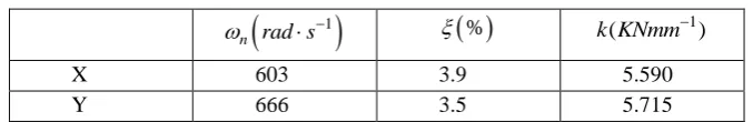
[image:8.479.63.402.362.417.2]

A practical 3-tooth, 30 mm diameter end mill with the modal characteristics in the X and Y directions corresponding to table 1 is chosen for this example. The work-piece is a rigid aluminium block whose specific cutting energy is k_t 600kN mm 1and the proportional factor is taken to bekr 0.07.

Table 1 Modal parameters of the tool.



1



n rad s

 _ 

_

 

_{% k KNmm(} 1₎

X 603 3.9 5.590

Y 666 3.5 5.715

For the model reference control, the transfer function of equation 6 has a cutting pressure selected to be constant and equal to 1200N mm 2 in all range of cutting parameters, the CNC

time constant,  m 0.1msand,  c 1N St s . The continuous model reference system of the

adaptive control is chosen to be a typical continuous second order plant with



0.75 and





2.5 4

n T



  , where Tis the sampling period. Also, it is desirable for the reference force to be maintained at1200N.

For example purposes, it is supposed that the following two cutting parameters represent two Pareto optimal fronts, Ss₁2710andadc10.3710, as point 1, andSs13260,

1 0.4127

dc

a  , as point 2. A more in-depth explanation of how to obtain Pareto optimal cutting parameters is provided by Rubio et al. [7].

Regarding the control scheme, it is taken into account that







1, 0.7, 0.5, 0.3, 0



, being

min 1

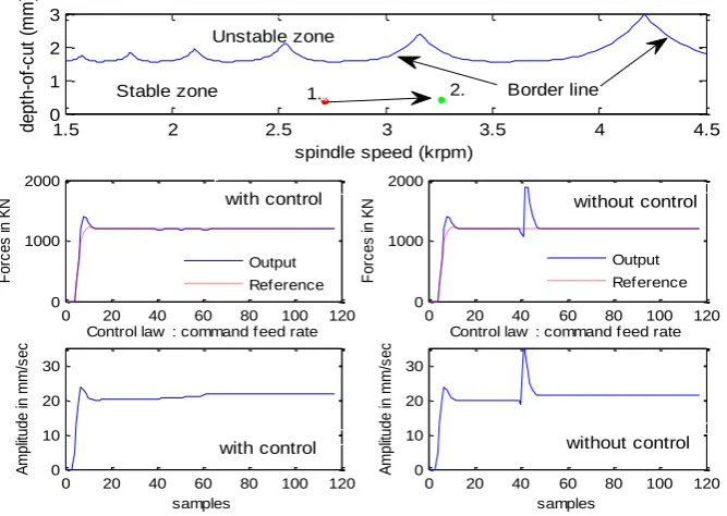
  and_max 0, corresponding with the points 1 and 2, respectively. Figure 3 depicts, from top to bottom, the stability lobes with the situation of the suggested Pareto optimal cutting parameters, the system output (resultant and reference forces) and the programmer feed rate when it is required to change the cutting parameter from point 1 to point 2 with and without applying the controller. The left hand figures show the outputs and control commands when the control scheme is applied. The right side corresponds to the case where the control scheme is not implemented. When the cutting conditions change, a peak appears in the resultant forces. This peak can lead to excessive wear and damage or even breakage of the tool or machine components. Moreover, those peaks can have a detrimental influence on the surface finish of the workpiece. In the proposed control algorithm the cutting forces are maintained constant by adjusting the feed rate according to the presented algorithm.

Then, as shown in figure 3, the Pareto optimal cutting parameters proposed by the self-optimized system are below the stability borderline in the stable zone. Furthermore, the presented controller is able to move automatically around the allowable cutting space parameter, keeping the forces below a prescribed upper limit bound while programming feasible command federate in spite of changes in cutting parameters.

[image:9.479.76.410.362.599.2]

Finally, the implemented controller can also be tuned in order to reduce the overshoot of the transitory state, which could also lead to damage or breakage of the tool or tool-holder and machine components and leave uneven surface finish.

Figure 3: Situation of the programmed cutting parameters in stability lobes, output force signal and control signal with and without applying the control

1.5 2 2.5 3 3.5 4 4.5

0 1 2 3

spindle speed (krpm)

d

e

p

th

-o

f-c

u

t

(m

m

)

0 20 40 60 80 100 120 0

1000 2000

F

o

rc

e

s

in

K

N

0 20 40 60 80 100 120 0

10 20 30

A

m

p

lit

u

d

e

in

m

m

/s

e

c

samples

Control law : command f eed rate

0 20 40 60 80 100 120 0

1000 2000

F

o

rc

e

s

in

K

N

0 20 40 60 80 100 120 0

10 20 30

A

m

p

lit

u

d

e

in

m

m

/s

e

c

samples

Control law : command f eed rate Output

Ref erence

Output Ref erence

1. 2.

Unstable zone

Stable zone

with control

with control

without control

6.

CONCLUSIONS

This paper proposes a novel control scheme for controlling cutting parameters in milling applications. It is composed of two levels. In the first level, the self-optimised cutting parameters layer comprises life of the tool, material remove rate, surface roughness and the robustness of the system. While the second layer, the parallel multi-estimation controller, provides an environment to control the milling process automatically under changes in cutting conditions. The change of the cutting parameters is scheduled by production requirements. For this purpose, an algorithm methodology is proposed in order to automatically adjust the parameter  choosing the most suitable controller among the set designed for each programmed optimal cutting parameters. The designed controller is able to smooth the transition between discrete control models and so reduce the peaks which appear when sudden changes are made in the cutting parameters.

The fundamental idea of the control system is to work automatically, with a simple interface with the operator, based around the admissible cutting parameter space given by the well-known stability lobes. First, the optimization cost function is used to obtain the cutting parameters according to multiple objectives optimization. Secondly, the adaptive control scheme proposes different control laws working in parallel to address the non-linear and changeable milling process. Finally, the supervisory scheme manages the system so it can work automatically in between optimal working points. Simulation results support the performance of the system.

ACKNOWLEDGEMENTS

The authors gratefully acknowledge the UK’s Engineering and Physical Science Research Council (EPSRC) funding of the EPSRC Centre for Innovative Manufacturing in Advance Metrology (Grant Ref: EP/I033424/1).

REFERENCES

[1] F. Cus, and J. Balic, “Optimization of cutting process by genetic algorithm approach,” Robotics and compute-integrated manufacturing , vol. 19, pp. 113-121, 2003.

[2] J.V. Abellan, F. Romeros, H.R. Siller, A. Estrud and C. Vila, "Adaptive control optimization of cutting parameters for high quality machining operations based on neural network," Advance in robotics, Automation and Control, I-tech, Vienna, Austria, 2008.

[3] U. Zuperl, and F. Cus, “Optimization of cutting conditions during cutting using neural networks,” Robotics and computer integrated manufacturing, vol. 19, no. 1-2, pp. 189-199, 2003.

[4] Y. Altintas, Manufacturing automation, Cambridge University Press, 2012.

[5] U. Zuperl, F. Cus and M. Milfelner, “Fuzzy control strategy for an adaptive force control of forces in milling processes,” Journal of Material Proccessing Technology, pp.1472-1478,2005.

[6] L. Rubio, M. De La Sen, and A. Bilbao-Guillerma, "Intelligent adaptive control of forces in milling processes," Proceedings of the 2007 IEEE Mediterranean Conference on Control, and Automation, pp. 1-6, 2007. [7] L.Rubio, M. De La Sen, A.P.Longstaff and S. Fletcher, “Model-based expert system to automatically adapt