Power analysis for generalized linear mixed models in ecology and evolution

Power analysis for generalized linear mixed models in

ecology and evolution

Paul C. D. Johnson

*, Sarah J. E. Barry

, Heather M. Ferguson

and Pie M

uller

€

1

_{Boyd Orr Centre for Population and Ecosystem Health, Institute of Biodiversity, Animal Health and Comparative Medicine,}

University of Glasgow, Graham Kerr Building, Glasgow G12 8QQ, UK;

Robertson Centre for Biostatistics, University of

Glasgow, Boyd Orr Building, Glasgow G12 8QQ, UK;

Department of Epidemiology and Public Health, Swiss Tropical and

Public Health Institute, Socinstrasse 57, PO Box, Basel CH-4002, Switzerland; and

University of Basel, Petersplatz 1, Basel

CH-4003, Switzerland

Summary

1.

‘Will my study answer my research question?’ is the most fundamental question a researcher can ask when

designing a study, yet when phrased in statistical terms

–

‘What is the power of my study?’ or ‘How precise will

my parameter estimate be?’

–

few researchers in ecology and evolution (EE) try to answer it, despite the

detrimen-tal consequences of performing under- or over-powered research. We suggest that this reluctance is due in large

part to the unsuitability of simple methods of power analysis (broadly defined as any attempt to quantify

pro-spectively the ‘informativeness’ of a study) for the complex models commonly used in EE research. With the aim

of encouraging the use of power analysis, we present simulation from generalized linear mixed models (GLMMs)

as a flexible and accessible approach to power analysis that can account for random effects, overdispersion and

diverse response distributions.

2.

We illustrate the benefits of simulation-based power analysis in two research scenarios: estimating the

preci-sion of a survey to estimate tick burdens on grouse chicks and estimating the power of a trial to compare the

effi-cacy of insecticide-treated nets in malaria mosquito control. We provide a freely available

R

function,

sim.glmm

,

for simulating from GLMMs.

3.

Analysis of simulated data revealed that the effects of accounting for realistic levels of random effects and

overdispersion on power and precision estimates were substantial, with correspondingly severe implications for

study design in the form of up to fivefold increases in sampling effort. We also show the utility of simulations for

identifying scenarios where GLMM-fitting methods can perform poorly.

4.

These results illustrate the inadequacy of standard analytical power analysis methods and the flexibility of

simulation-based power analysis for GLMMs. The wider use of these methods should contribute to improving

the quality of study design in EE.

Key-words:

experimental design, sample size, precision, generalized linear mixed model, random

effects, simulation, overdispersion, long-lasting insecticidal net

Introduction

‘Will my study answer my research question?’ is the most

fun-damental question a researcher can ask when designing a

study, yet when phrased in statistical terms

–

‘What is the

power of my study?’ or ‘How precise will my parameter

esti-mate be?’

–

few researchers in ecology and evolution (EE) try

to answer it (e.g. Taborsky 2010). Consequently many,

possi-bly most, studies are underpowered (Jennions & Møller 2003;

Smith, Hardy & Gammell 2011) and likely to be uninformative

or misleading (Ioannidis 2005). Failure to consider power can

also result in overpowered studies. Both under- and

overpow-ering waste resources and can raise ethical concerns (e.g. in

animal studies, by potentially causing needless suffering; and

in disease control by causing potentially promising control

methods to be prematurely dismissed). Hence, researchers

should take all reasonable steps to ensure sufficient, but not

wastefully excessive, power.

Power is defined as the probability of rejecting the null

hypothesis when it is false and is equal to one minus the type II

(false negative) error rate or 1-

b

. In other words, it is the

proba-bility of detecting an effect, given that it exists. It depends on

the sample size, the effect size, the amount of variability in the

response variable and the significance level. Generally, the aim

of a power analysis is to predict the power of a particular

experimental design, or the sample size required to achieve an

acceptable level of power [80% power is conventionally

deemed adequate, although often without justification (Di

Stefano 2003)]. Power analysis therefore exists within the

framework of null hypothesis significance testing (NHST). In

this article, we define power analysis more broadly as any

attempt to quantify prospectively the ‘informativeness’ of a

study (Bolker 2008; Cumming 2013). This definition of power

analysis covers, for example, predicting the precision of an

esti-mate, and could be applied within alternative inference

frame-works such as Bayesian or information theoretic.

A major obstacle to power analysis is that standard

meth-ods are suitable for only the simplest statistical analyses,

such as comparing means using

t

-tests or

, or

propor-tions using

v

tests, and are inadequate when confronted

with the more complex analyses generally required to

ana-lyse ecological data. Such anaana-lyses commonly accommodate

multiple sources of random variation (e.g. within and

between study sites), where random effects models (also

known as mixed effects models) are recommended. In

addi-tion, response measures such as counts that are common in

EE are not readily shoehorned into

t

-tests,

or

v

tests,

and consequently, the associated power analysis methods

are inappropriate. Neither random effects nor count

responses are handled in relatively sophisticated power

analysis software such as

*

(Faul

et al.

2007).

The generalized linear mixed model (GLMM) is an analysis

framework widely used in EE that can accommodate these

complexities. GLMMs allow modelling of diverse response

distributions and multiple sources of random variation termed

random effects, both of which are common in EE (Bolker

et al.

2009; Zuur, Hilbe & Leno 2013). Although analytical

formulae for estimating power are available for the simplest

Gaussian GLMMs (Snijders & Bosker 1993), more general

formulae are not available. A more flexible approach is to use

Monte Carlo simulation (Thomas & Juanes 1996).

Simula-tion-based power analysis has many additional advantages

over analytical power analysis, beyond its greater flexibility. It

is more accurate, conceptually simpler and easy to extend

beyond hypothesis testing (Bolker 2008). Simulation-based

power analysis methods are available for Gaussian GLMMs

(Martin

et al.

2011), but there is a lack of guidance and

soft-ware facilitating power analysis for scenarios with

non-Gauss-ian responses and more complex random effect structures.

The first aim of this study is to illustrate the value of power

analysis in the broad sense of predicting the informativeness of

a study. The second is to present simulation from GLMMs as

a flexible and accessible power analysis method, with examples

taken from two ecological systems where standard power

analysis methods are inadequate: estimating tick density on

game birds and assessment of insecticide-treated nets for

malaria mosquito control.

Materials and methods

P O W E R AN A L Y S IS US IN G S I M U LA T IO N

Estimating the power of a test of a null hypothesis by simulation requires the following steps (Bolker 2008):

1.Simulate many data sets assuming that the alternative hypothesis is true, that is, the effect of interest is not zero. ‘Many’ means enough to give an adequately precise power estimate. As a guide, with 100 simulations and 80% power, the power estimate will fall within 72– 88% with 95% probability, while using 1000 simulations will reduce this range to 775–824%.

2. Using each simulated data set, perform a statistical test of the null hypothesis that the effect size is zero.

3. Calculate the proportion of simulated data sets in which the null hypothesis was rejected. This proportion is the power estimate. The effect of different designs and assumptions (e.g. sample size, effect size, random effect variances) on power can be explored by repeating steps 1_–3 across a range of realistic scenarios.

This scheme can be easily adapted to quantify the informativeness of a study in the broader sense of power analysis defined above. The preci-sion of an effect estimate could be predicted by averaging CI width over the simulated data sets, or, in an information theoretic framework (Burnham & Anderson 2001), the expected difference in the Akaike information criterion (AIC) between models could be estimated.

A N O V E R V I E W O F G L M M S

We focus on counts and proportions because these are common types of response data in EE. First, we introduce generalized linear models (GLMs). Like a standard linear regression model (LM), a GLM mod-els, the relationship between the response of theith observation,yi, and

a set ofppredictor variables or covariates,x1i,. . .,xpiviapregression

coefficients,b1,. . .,bp. Unlike a LM, the response can follow

distribu-tions other than normal (Gaussian), including binomial, Poisson and negative binomial. As in standard linear regression, the predictors, weighted by the regression coefficients, are summed to form the linear predictor,

gi¼b0þ

Xp

m¼1

bmxmi;

where_b0is the intercept. The expected value ofyiand the linear

predic-tor,gi, are related through the link function. For example, in a Poisson

GLM, whereyiPoisð Þki andkiis the expected value ofyi, the link

function isgi=log(ki) (where ‘log’ means the natural logarithm, loge,

throughout the text). If the responses were binomially distributed with

niBernoulli trials andpiprobability of success in each trial, that is

yiBinom nði;piÞ, then we would model the responses using a binomial GLM, usually with a logit (log of the odds) link function,

gi¼logitð Þ pi log

pi 1pi

:

There is often a need to account for additional sources of random variation, for example where observations are clustered within study sites, or where multiple observations are taken over time on each study subject. In such data sets, the assumption of the GLM that theyivalues

are conditionally independent (i.e. independent after adjusting for the effects of covariates) is violated, because clustered observations are cor-related. To account for these correlations, a random effect can be added to the linear predictor, allowing each cluster (e.g. site or individual) to have its own mean value. The resulting model is a GLMM. In the example of intersite variation, we are now modelling the response of theith observation in thejth site,yij. The only change to the model is

the addition of a single random effect,cj, to the linear predictor,

repre-senting the ‘effect’ of thejth site. Now

gij¼b0þ

Xp

m¼1

bmxmijþcj;

wherec_jN 0;r2 c

sites. Multiple random effects can be included, and random effects can take more complex forms that allow greater flexibility in modelling cor-relations between observations (e.g. due to familial cor-relationships or proximity in space or time). GLMMs in which regression coefficients, or slopes, are allowed to vary randomly between clusters are termed random slopes GLMMs. Random intercepts-and-slopes models have been applied to modelling inter-individual variation in regression coefficients both where this variation is the focus of enquiry, as in random regression models (Nussey, Wilson & Brommer 2007), and where it is a nuisance variable that must nevertheless be modelled to guard against overconfident inference (Schielzeth & Forstmeier 2009; Barret al.2013). Power analysis for random inter-cepts-and-slopes GLMMs is beyond the scope of this article, although simulation-based power analysis methods have been developed for

Gaussian random regression models and implemented in thePAMM

package for theRstatistical environment (Martinet al.2011).

S IM UL A T ING F RO M A GL MM

The first step of simulation-based power analysis is to simulate a large number of data sets. When simulating responses from a GLMM, we must assume values for the intercept and the regression coefficients (the fixed effects) and the variances and covariances of the random effects. Estimates of these parameters, or a range of plausible values, will some-times be available from previous studies; otherwise, a pilot study should be conducted. If no data are available, a plausible range of parameter values could, in some cases and with careful justification, be assumed based on knowledge of the study system.

While designing a study, we will often suspect which predictor vari-ables are most strongly related to the response variable. To simulate responses from a GLMM, we must make assumptions about these rela-tionships, which amounts to assuming values for each of the_bm. The

interpretation of thebmdepends on the type of GLMM. In a Poisson

GLMM, they are log relative abundances, or rate ratios, and in a bino-mial GLMM with a logit link they are log odds ratios. Generally, we will have little knowledge of the size of the effect that is the focus of the study, but this is not an obstacle to power analysis because the study should be powered to detect thesmallest biologically meaningful effect, which is purely a question of scientific judgement (see Discussion).

In addition to thebm, we must assume a value for the intercept,b0,

which is the expected value ofgijwhere all thexmijare zero. If setting

thexmijto zero is meaningful–for example, if thexmijrepresent time

from the start of the study, or all but one of the levels of a categorical variable–then the intercept is the value of the linear predictor at base-line or in the reference category, respectively. Thus, in a Poisson GLMM,b0is the log expected count in the baseline or reference

cate-gory, and in a binomial GLMM with a logit link,b0is the logit expected

proportion or prevalence in the baseline or reference category. Next, we must make assumptions about the random effects. In the example of a single between-site random effect, only a single variance needs to be assumed. In more complex models, such as random inter-cepts-and-slopes, multiple random effects and their covariances might need to be considered, but here, we consider only uncorrelated random effects and so assume zero covariance. The value assumed for a random effect variance should be based on an estimate from previous studies or pilot data, where available. Uncertainty around variance estimates can be considerable, and the sensitivity of the power analysis to this uncer-tainty can be assessed by repeating the power analysis across a range of plausible variance values in place of the point estimate.

An additional source of variation that needs to be considered is over-dispersion. Overdispersion is variation exceeding what would be

expected from a given distribution and can be thought of as unex-plained variation. For example, a Poisson distribution with meankalso has variancek. If the variance in a set of counts is greater than the mean then they will not fit a Poisson distribution and are overdispersed. Simi-larly, a set of binomial responses is overdispersed if the variance exceeds

np(1–p), wherenis the number of trials,n>1, andpis the probability of success in each trial. Overdispersion in a GLMM fit can be artefactu-al or reartefactu-al (Zuur, Hilbe & Leno 2013). Artefactuartefactu-al overdispersion arises from model misspecification and has several potential causes including missing or poorly modelled covariates, interactions or random effects; wrong choice of distribution or link function; outliers; and zero-infla-tion. Once these potential causes have been investigated and remedied, any overdispersion that remains is ‘real’ and should be modelled. Fit-ting a Poisson or binomial GLMM that does not allow for overdisper-sion is equivalent to assuming that all of the variation that does not arise from the Poisson or binomial distribution is explained by the fixed and random effects. Biological data rarely justify this assumption, so overdispersion should be considered as a matter of course (but note that overdispersion does not apply to the normal distribution because the variance is independent of the mean). While EE researchers have long been alert to overdispersion in count data (Bliss & Fisher 1953; Eberhardt 1978; O’Hara & Kotze 2010), awareness of overdispersion in binomial data (Crowder 1978; Warton & Hui 2011) is comparatively limited. Various methods of accounting for overdispersion are avail-able, including negative binomial and quasi-Poisson for counts, and beta-binomial and quasi-binomial for binomial data (Bolkeret al.

2009; O’Hara & Kotze 2010; Warton & Hui 2011; Zuur, Hilbe & Leno 2013). Here, we model overdispersion in both Poisson and binomial GLMMs by adding a normally distributed random intercept,eij, to the

linear predictor of each observation, giving

gij¼b0þ

Xp

m¼1

bmxmijþcjþeij;

where eijNð0;r2_eÞ(Elstonet al. 2001; Warton & Hui 2011). By absorbing excess (i.e. unexplained) variation, this random effect per-forms the same role as the residual error term in a linear regression model. Like the random effects variances, the value assumed for the overdispersion variance in the simulation model should be estimated from pilot data.

E X A M P L E S

We illustrate power analysis for GLMMs with two contrasting exam-ples. In the first, the responses are counts and the random effects are nested. This example is a power analysis in the broad sense because the aim is to predict not power but the precision of an estimate in terms of confidence interval (CI) width. The second example, in which the responses are binomial and the random effects are crossed, is a narrow sense power analysis where the aim is to estimate the power of a hypothesis test.

Count response example: estimating tick burden on grouse

chicks

This example is based on an analysis of tick burdens recorded on grouse chicks on an Aberdeenshire moor from 1995 to 1997 (Elston

et al.2001). Our sampling scheme is a simplified version of Elstonet al.

95% confidence limits to the estimate (it is necessary to average because a CI for a Poisson mean estimated from a GLM or GLMM is asym-metrical, due to having been back-transformed from a symmetrical 95% CI on log scale). For example, a 95% CI of 8 to 13 around an esti-mate of 10 ticks per chick has confidence limits that are on average (2+3)/2=25 units from the estimate, giving an adequately precise margin of error of 25/10=25%. The aim of the power analysis is to determine the sampling effort required to give adequate precision. Because we are aiming for 25%expectedmargin of error, and the mar-gin of error is subject to sampling error, we are implicitly prepared to accept a 50% risk of a higher margin of error. If estimating tick burden with poorer precision were expected to have undesirable consequences, the specification could be changed to give greater confidence (e.g. 80% or 90%) of adequate precision. It would be straightforward to adapt the power analysis to estimate the additional sampling effort required.

Predicting the precision to which we can measure tick burden requires the following assumptions (Table 1):

1.The mean tick burden per chick.Mean tick burden is highly variable, ranging from 12 to 111 over the three years. To account for this uncertainty, we simulated mean tick burdens of 1, 5 and 10 ticks per chick.

2.The effect sizes of factors affecting tick burden.Tick burden varies substantially between locations, between broods within locations and between chicks within broods (Elstonet al.2001). We modelled variation between locations, broods and chicks with a random effect at each hierarchical level. These random effects are nested, because each brood belongs to only one location, and each chick to only one brood. As each chick provided only one tick count, the chick-level random effect models overdispersion. We simulated na€ıve (zero) and pessimistic (high) variances for each hierarchical level (Table 1). Pessimistic random effect variances were selected by choosing values towards the upper ends of the 95% CIs in Table 1 of Elstonet al.

(2001).In the interests of simplicity, we did not include any fixed

effects in the simulation model. Fixed effects are introduced in the second example.

3. The number of chicks sampled.We assumed that every brood con-sisted of three chicks and that two broods were sampled at every location. We varied sampling effort by increasing the number of locations sampled from 10 to 200.

The tick burden on theith chick from thejth brood in thekth loca-tion,yijk, was modelled as Poisson distributed, that isyijkPoiskijk . The expected log tick burden, log(kijk), is

gijk¼b0þlkþbjkþeijk;

where_b0is the global mean log tick burden, andlk,bjkandeijkare the

location, brood and chick random effects, which are normally distrib-uted with zero means and variancesr2

l,r2bandr2e, respectively.

Binomial response example: comparing mortality of malaria

mosquitoes exposed to long-lasting insecticidal nets

Long-lasting insecticidal nets (LLINs) are made of fabric with incorpo-rated insecticide which maintains residual activity for several years. LLINs are a key intervention against malaria (Roll Back Malaria Part-nership 2008; World Health Organization 2013b). They provide per-sonal protection from malaria mosquitoes by constituting a physical barrier and community protection by killing potentially infectious mos-quitoes upon contact (Lengeler 2004). To evaluate their insecticidal activity, LLINs are tested in standardized experimental huts (World Health Organization 2013a) against free-flying, wild mosquitoes. The mosquitoes can enter but not leave the huts, allowing assessment of LLIN efficacy under controlled conditions. Despite their importance in large-scale malaria prevention programs, power analysis has not gener-ally been performed for LLIN hut trials. Power analysis for LLIN hut trials is hindered by the difficulty of accounting for the effects of multi-ple sources of variation in mosquito mortality, including variation between huts and over time. We show how simulation can be used to account for these complexities.

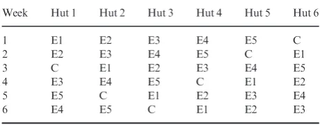
The aim is to optimize the design of an experimental hut trial com-paring mortality in the malaria vectorAnopheles gambiaeamong differ-ent types of LLIN. This is achieved by estimating power across a realistic range of assumptions and designs, identifying those that give adequate (≥80%) power. In this example, six types of LLIN are to be tested in six experimental huts, in accordance with the World Health Organization Pesticide Evaluation Scheme (WHOPES) guidelines (World Health Organization 2013a). To prevent confounding of hut and net effects, the LLIN types are rotated through the huts weekly, so that after six weeks, one Latin square rotation has been completed, with each LLIN type having passed one week in each hut (Table 2). Simple rotation, where net type E2 always follows E1, etc, would lead to confounding between LLIN type and any carry-over effects, so Table 2 presents a design balanced against such effects, where each net type follows each other net type only once (Williams 1949). Data are collected on six nights per week. Nets are replaced after each night so that six replicate nets of each type are used per week. The outcome of interest is mosquito mortality, calculated as the proportion of mosqui-toes entering the hut at night that are found dead in the morning or in the following 24 hours. Any mosquito found alive inside the hut is transferred to an insectary and mortality recorded after a holding per-iod of 24 hours. We aim to estimate the number of six-week Latin square rotations that will be required to give adequate power.

Performing the power analysis requires the following information:

1. The primary aim of the experiment and the consequent primary analysis.This example follows the standard WHOPES design in

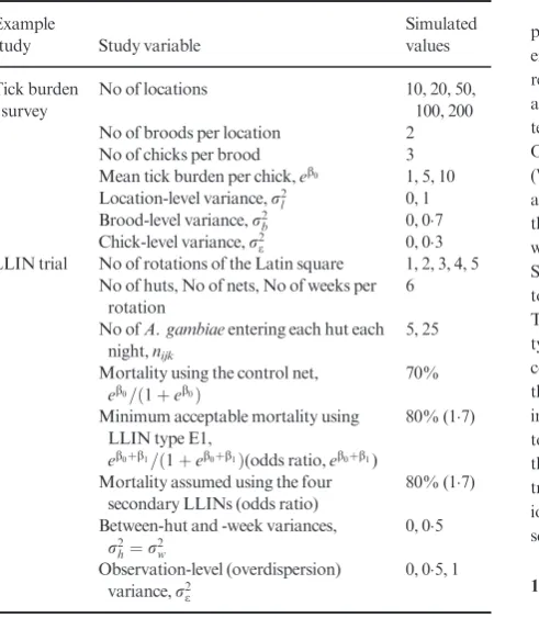
Table 1.Study design choices and effect parameter assumptions for the two example studies

Example

study Study variable

Simulated values

Tick burden survey

No of locations 10, 20, 50,

100, 200

No of broods per location 2

No of chicks per brood 3

Mean tick burden per chick,eb0 _{1, 5, 10}

Location-level variance,r2

l 0, 1

Brood-level variance,r2

b 0, 07

Chick-level variance,r2

e 0, 03

LLIN trial No of rotations of the Latin square 1, 2, 3, 4, 5

No of huts, No of nets, No of weeks per rotation

6

No ofA. gambiaeentering each hut each night,nijk

5, 25

Mortality using the control net,

eb0=ð₁þ_eb0Þ

70%

Minimum acceptable mortality using LLIN type E1,

eb0þb1=ð₁þ_eb0þb1Þ_{(odds ratio,e}b0þb1₎

80% (17)

Mortality assumed using the four secondary LLINs (odds ratio)

80% (17)

Between-hut and -week variances,

r2

h¼r2w

0, 05

Observation-level (overdispersion) variance,r2

e

which multiple net types are tested simultaneously, allowing multiple secondary research questions to be asked. This power analysis, however, is concerned only with the primary aim of the study, which is to evaluate the efficacy, in terms of mosquito mortal-ity, of an experimental LLIN (labelled E1 in Table 2) compared with a positive control LLIN (labelled C in Table 2), which would typically be a WHOPES-recommended LLIN (World Health Orga-nization 2013a). The primary analysis will be a two-tailed test of the null hypothesis that the control and E1 LLIN types cause the same mortality. The other four experimental LLIN types (labelled E2 to E5 in Table 2) do not feature in the primary analysis, but are included in the simulation because they contribute to the estimation of the hut effect.

2. The number of mosquitoes in each treatment group. The total number ofA. gambiaeexpected to be sampled in each of the six treatment groups,n, is the product of the number of nights per week when mosquitoes are collected (six), the number of weeks in one rotation (six), the number of mosquitoes caught per night in each hut (nm)

and the duration of the study in number of six-week rotations (nr),

so thatn =36nmnrThe number of mosquitoes entering a hut is

dif-ficult to predict. We investigated low (nm= 5) and high (nm= 25)

A. gambiaeabundance, which is a realistic range (Malima et al.

2008; Winkleret al.2012; Nguforet al.2014). The study was run fornr=1,. . .5 complete six-week rotations of the nets through the

huts.

3. The mortality in huts using the positive control LLIN type. We assumed a realistic mortality rate of 70% (Malimaet al.2008; Win-kleret al.2012; Nguforet al.2014).

4. The size of the smallest treatment effect worth detecting (the sensitiv-ity of the study). We considered mortality of at least 80% using LLIN type E1 to represent a worthwhile improvement in efficacy relative to the control LLIN. This treatment effect can be repre-sented as an odds ratio of 80₇₀=₌20₃₀1:7. For simplicity, we also assumed 80% mortality with the four secondary LLINs.

5. The impact of non-treatment factors on mortality. Variation in mor-tality among huts and over time is expected, which we simulated as simple random effects between huts and between weeks. The justifi-cation for modelling week-to-week variation as random rather than fixed is that we cannot predict the form of the relationship between mortality and time, so any choice of fixed effect form would be arbi-trary. A random effect is a simple and conservative way of modelling week-to-week variation without foreknowledge of its nature. The hut and week random effects arecompletely crossed, because data are collected from each hut during each week (Table 2). Between-hut and between-week random effect variances of up to 05 are plau-sible based on analysis data from Winkleret al.(2012). In order to limit the number of parameter combinations, we set the variances between huts and between weeks to be equal. We simulated two hut

and week random effect scenarios:r2

h¼r2w¼0, representing a

na€ıve assumption that mortality does not vary between huts or over weeks and a more realistic assumption ofr2

h¼r2w¼0:5. Another potential source of variation in mortality is the six sleepers who rotate nightly through the huts, in accordance with the WHOPES guidelines (World Health Organization 2013a). We ignored this aspect here for the sake of simplicity and assumed that sleepers have no influence on mosquito mortality.

6. The amount of unexplained variation in mortality (overdispersion). We explored three scenarios: a na€ıve assumption of no overdisper-sion (r2

e¼0); realistic overdispersion (r2e¼0:5, similar to the esti-mated value of 04 from analysis of Winkleret al.(2012)); and a pessimistic assumption of strong overdispersion (r2

e¼1).

These assumptions are summarized in Table 1. The GLMM that fits the design described above models the number of dead mosquitoes recorded on theith night from thejth hut in thekth week among the

nijkmosquitoes entering the hut,yijk, as binomially distributed, that is

yijkBinom nijk;pijk

. The log odds of mortality, logit pijk , can be modelled as

gijk¼b0þ

X5

m¼1

bmxmjkþhjþwkþeijk;

where the intercept,b0, is the predicted log odds of mortality when

using the positive control net (type C) andbmis the log odds ratios

representing the difference in the log odds of mortality between the

mth of the five experimental nets (types E1-E5) and the control net. The covariatexmjkis an indicator, or dummy variable, that takes the

value 1 when themth of the five experimental nets is in use and 0 otherwise. For example, when the first experimental net, type E1, is in use,x1jk=1 andx2jk=x3jk=x4jk=x5jk=0, so the log odds of

mor-tality on the ith night in the jth hut in the kth week is

gijk=b0+b1+hj+wk+eijk. The hut random effect,hj, the week random

effect,wk, and the observation-level random effect,eijk, are normally

distributed with zero mean and variancesr2

h,r2wandr2e, respectively.

For simplicity, we simulatednijkas a constant, although in reality this

quantity is random. Simulations of nijk as random indicated that

power was not sensitive to this simplification (data not shown).

S IM UL A T IO N M ET HO D S

All combinations of the parameter values in Table 1 were simulated, giving a total of 120 scenarios for the tick burden survey and 60 for the LLIN trial. For each example study, 1000 data sets were simulated from each scenario. The responses were simulated using a function,

sim.glmm, for the statistical environmentR(R Core Team 2014) which is freely available at https://github.com/pcdjohnson/sim.glmm. The function simulates from Gaussian, Poisson, binomial and negative

binomial GLMMs; a tutorial is provided as Appendix S1. The

simu-late.merModfunction included in recent versions (_≥10) of thelme4 R

package has similar functionality (Bateset al.2014).

The next step is to analyse the simulated data set. Ideally, this should be done using the same methods that would be used for the real data, but this is problematic for non-Gaussian GLMMs because the most reliable method for estimatingP-values and CIs, parametric bootstrap-ping (Faraway 2005), is prohibitively slow for multiple simulations. We have therefore taken the approach of using fast, approximate methods to estimateP-values and CIs, while monitoring performance to identify scenarios where precision and power estimates are unacceptably inac-curate. In such cases, the more accurate methods should be used despite their slowness (see Appendix S1). The definition of ‘unacceptably inac-curate’ is subjective, but would cover, for example, a 95% CI that included the true value with only 85% probability. Small biases are acceptable because power analysis is an inherently approximate

Table 2. Latin square design for trialling one control (C) and five experimental (E1 to E5) types of long-lasting insecticidal net, rotated through six huts over six weeks according to a design balanced against carry-over effects (Williams 1949)

Week Hut 1 Hut 2 Hut 3 Hut 4 Hut 5 Hut 6

1 E1 E2 E3 E4 E5 C

2 E2 E3 E4 E5 C E1

3 C E1 E2 E3 E4 E5

4 E3 E4 E5 C E1 E2

5 E5 C E1 E2 E3 E4

procedure, with results being strongly dependent on uncertain assump-tions. However, in an analysis of real data, where computation time is much shorter because the analysis need be run only once, researchers should use the most accurate methods available, such as parametric bootstrapping (Faraway 2005).

We analysed each simulated data set by fitting the GLMM from which it was simulated using thelme4package (Bateset al.2014) for

R. Wald z CIs around tick burden estimates were calculated as

expðb^₀1:96s_b0Þ;wheres_b0is the estimated standard error of^b₀and 196 is the 975th percentile of the standard normal distribution. The null hypothesis of equal mortality between the standard (C) and experi-mental (E1) net types was tested using a Waldv2-test with one degree of freedom for theb1parameter, with the null hypothesis being rejected

whenP<005. In GLMMs with overdispersion, Wald z CIs and

v2

-tests are expected to give overconfident 95% CI coverage (i.e. true confidence being<95%) and inflated type I error rate (Bolker et al.

2009), leading to overestimation of precision and power. We therefore monitored type I error rate (the proportion of null hypotheses rejected when the null hypothesis is true) and 95% CI coverage (the proportion of 95% CIs that include the true effect size). We also monitored bias in parameter estimation.

Power to detect the difference in mosquito mortality between the two LLIN types was estimated as the proportion of the 1000 simu-lated data sets in which the null hypothesis was rejected. Margin of error in the tick burden example was averaged over the 1000 simulated data sets. Mean computation time per 1000 simulations was 88 min

for the binomial example and 20 min for the Poisson data

exam-ple using a 27 GHz Intel Core i7 processor, parallelizing across 8 processor cores.

Results

C O U N T R E S P O N S E E X A M P L E: E ST IM A T I N G T I C K B U R D E N O N G R O U S E C H I C K S

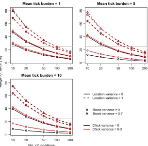
The precision of the estimates was greatly reduced by allowing

counts of ticks on chicks to be non-independent within broods

and locations (Fig. 1). The analysis assuming independence

among chicks (random effect and overdispersion variances

=

0;

black circles and solid lines in Fig. 1) suggests that sampling only

20 locations will be sufficient to keep the expected margin of error

within

25% (below the grey line in Fig. 1) even at the lowest

mean tick burden. Under more realistic assumptions that allow

tick burdens to be correlated at the chick, brood and location

lev-els (red triangles and dashed lines in Fig. 1), the margin of error

doubles. The impact on the study design of considering random

effects is severe. A fivefold increase in sampling effort to 100

loca-tions is required to achieve the desired level of precision,

regard-less of mean tick burden. In contrast to the binomial example (see

below), random effects at all levels, not just overdispersion,

con-tribute to reducing precision.

Of the three random effects, the location effect had the

largest impact on precision. The brood effect also

substan-tially reduced precision, while the effect of the chick (or

over-dispersion) random effect was generally small. We confirmed

that this effect was not simply due to location having the

strongest random effect (

r

l

¼

1) by repeating the simulations

with random effects variances at all levels set to 0

5 (data not

shown).

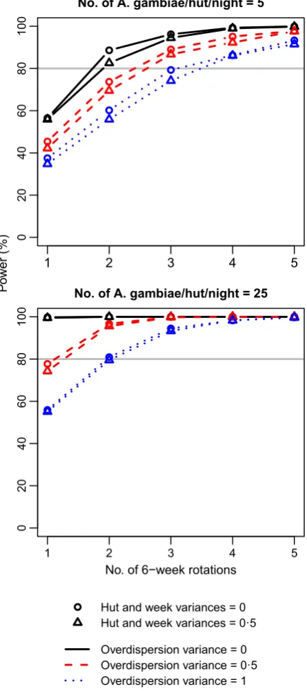
B IN O M I A L R ES P O N S E E X A M P LE : C O M P A R ING MO RTALITY OF MALARIA MOSQUITO ES EXPOSED TO L O N G - L A S T I N G IN S E C T IC I D A L NE T S

Standard power calculators ignore sources of

non-indepen-dence such as the hut, week and overdispersion effects

con-sidered here, producing power estimates equivalent to the

black circles in Fig. 2 (i.e. variance for each random effect

was set to 0). This was verified by estimating power

assum-ing independent observations usassum-ing

*

(Faul

et al.

2007) and the

power.prop.test

function in

R

. Ignoring these

effects and assuming that on average only five

A. gambiae

will enter each hut each night, 56% power is achieved after

one rotation, 89% after two and 96% after three. Under the

high abundance scenario of 25

A. gambiae

per hut per night

on average, a single rotation of the Latin square is sufficient

to give 100% power. Thus, a cautious researcher might plan

to run the experiment over two 6-week rotations to insure

against low

A. gambiae

abundance. How does consideration

of the random effects change this conclusion? Power is

decreased slightly by the hut and week random effects

(trian-gles in Fig. 2), but is markedly reduced by overdispersion

(red dashed and blue dotted lines). When mosquito

abun-dance is low, realistic overdispersion (

r

e

¼

0

:

5; red dashed

lines) necessitates three rotations to achieve at least 80%

power, and strong overdispersion (

r

e

¼

1; blue dotted lines)

requires three to four rotations. At higher abundance, and

assuming realistic overdispersion (red dashed lines), power

falls just short of the 80% threshold after one rotation so

that two rotations are required to exceed it. Two rotations

are also just sufficient to achieve 80% power assuming

strong overdispersion (blue dotted lines). Thus, consideration

of non-independence, and overdispersion in particular,

would motivate extending the duration of the trial by 50

–

100%, with important implications for planning and

resourc-ing the study.

An alternative to extending the duration of the trial would

be to focus effort on the two net types of primary interest, the

control net and the primary experimental net, by reducing the

number of net types trialed. For example, if only the control

net and two experimental nets were trialed, the number of

observations per net type could be doubled. We found that this

gives equivalent power to doubling the duration of the trial

(data not shown).

B IA S A N D C O N F ID E N C E IN T E R V A L C O V E R A G E

On average, CI coverage tended to be slightly overconfident

(i.e. too narrow) in the count example and accurate in the

binomial example (Fig. S3 and S4). Mean 95% CI coverage

across all scenarios was 93

4% for the tick burden estimates

and 94

4% for the mortality odds ratio estimates. Coverage of

the odds ratio estimate under the null hypothesis of no

differ-ence between the nets (odds ratio

=

1), which is equivalent to

one minus the type I error rate, was similar to coverage under

the alternative hypothesis (Fig. S5), with mean coverage of

94

6%, or, equivalently, a type I error rate of 5

4%, close to

the nominal value of 5%. Under both the null and

alterna-tive hypotheses, scenarios that gave significantly low coverage

(

<

93%) tended to be those where

A. gambiae

abundance was

low and overdispersion was at realistic (

r

e

¼

0

:

5) or strong

(

r

e

¼

1) levels. CI coverage in the tick abundance example

fol-lowed a similar pattern to that shown by bias, tending to be

more problematic when sampling effort was low, with

cover-age typically around 90% in scenarios where the total number

of ticks was low, either due to low tick abundance or low

sam-ple size.

Discussion

The key question to answer when assessing the utility of the

power analysis methods presented here is: will they help

researchers in ecology and evolution to design better studies?

To do this, they must be (i) substantially more accurate than

conventional power analysis methods to justify the extra time

and effort required and (ii) reasonably straightforward to use.

On the first point, consideration of random effects had a major

impact on study design in both of the examples, motivating an

increase in sampling effort of up to twofold in the binomial

example and fivefold in the count example. On the second

point, although our experience is that the perceived complexity

of simulation from GLMMs can be intimidating, we argue

that the methods presented here are no more complex

concep-tually, and only slightly more challenging technically, than

fit-ting and interprefit-ting a GLMM.

The methods presented here are flexible because GLMMs

are flexible. Their flexibility is illustrated by the contrast

between the two example studies: binomial vs. count responses;

crossed vs. nested random effects; inference via NHST vs.

con-fidence interval estimation; experimental vs. observational

study design. This flexibility encompasses many common

sim-pler analyses which can also be simulated as GLMMs,

includ-ing linear mixed effects regression, GLMs, linear regression,

ANOVA

and

t

-test. More complex models can also be simulated.

For example, zero-inflated count models (Zuur, Saveliev &

Ieno 2012) could be simulated as the product of binary and

Poisson or negative binomial responses.

What do these results tell us about the impact of random

effects and overdispersion on power and precision? Although

we cannot generalize beyond the two examples, the results

show that the effects of random variation on power and

preci-sion can depend on the specific study scenario. In the binomial

example, overdispersion was the principal drain on power,

while the higher level random effects (hut and week) had

little impact. An implication of this observation is that when

10 20 50 100 200

0

20

40

60

80

10 20 50 100 200

02

0

4

0

6

0

8

0

10 20 50 100 200

0

2

04

06

08

0

No. of locations

Margin of error (%)

Location variance = 0 Location variance = 1

Brood variance = 0 Brood variance = 0·7

Chick variance = 0 Chick variance = 0·3 Fig. 1. The relationship between margin of

error in tick burden estimates and number of locations sampled. Margin of error was aver-aged over 1000 data sets simulated under sce-narios that varied in mean tick burden and the degree of variation in mean tick burden at the location, brood and individual chick levels. The grey line shows the target margin of error

overdispersion is present, power can depend not just on the

quantity of data (here total mosquito numbers), but also on

how it is collected. For example, running the trial for one

rota-tion catching 25 mosquitoes per hut per night yields exactly the

same number of mosquitoes per treatment arm, 150, as

run-ning five rotations with an abundance of 5 mosquitoes per hut

per night, yet in the presence of overdispersion, the latter

sce-nario gives considerably more power (Fig. 2). In the count

example, by contrast, overdispersion had relatively little

impact compared with the higher level random effects. The

critical factor in determining precision was the variance at the

highest level, among locations. This effect has been observed in

multilevel LMMs, where power is limited principally by the

highest level sample size (Maas & Hox 2005; Snijders 2005).

The contrasting patterns between the two examples presented

emphasize the unpredictability of the results of power analysis

when there are multiple sources of variation, and the necessity

of tailoring power analysis to apply to specific study designs

and study systems.

Although we have shown that ignoring the influence of

ran-dom effects and overdispersion on power analysis can grossly

mislead study design, we are not suggesting that many

researchers would be so na

€

ıve. EE researchers are generally

alert to the impact of non-independence and overdispersion on

inference, as evidenced by the widespread awareness of

pseu-doreplication (Hurlbert 1984) and the popularity of GLMMs

(Bolker

et al.

2009). It is more likely that they would not do a

power analysis at all. Why not? Our experience is that there is

simply not a culture of performing power analysis. This

suppo-sition is supported by the fact that few EE journals recommend

that authors use power analysis. Together the Ecological

Soci-ety of America (ESA;

n

=

3 journals), the British Ecological

Society (BES;

n

=

4), the European Society for Evolutionary

Biology (ESEB;

n

=

1) and the Society for the Study of

Evolu-tion (SSE;

n

=

1) publish nine of the most prominent primary

research journals in EE. Only the ESA mentions power

analy-sis in its guidance for authors, in tentatively supportive terms

[‘Power analyses

. . .

occasionally can be very useful’

(Ecologi-cal Society of America Statisti(Ecologi-cal Ecology Section 2012)], while

none of the other journals mention the topic at all in their

guid-ance. If journals are committed to raising the quality of the

sci-ence they publish, journal editors should encourage and, where

appropriate, require authors to include an

a priori

power

analysis, or at least a justification of its omission. Although we

have no objective evidence identifying other barriers to power

analysis, in our experience these include a belief that power

analysis cannot be extended beyond NHST inference; a lack of

available power analysis methods for complex analyses; a lack

of technical knowledge of even simple power analyses; and the

perceived difficulty of defining a biologically meaningful effect

size.

We argue that the last of these obstacles arises from a

misun-derstanding of the concept of a biologically meaningful effect

size. This obstacle is (in our experience) frequently expressed as

a question: ‘How can I power my study to detect an effect size

of which I have no knowledge?’ The answer is that the study

should be powered to detect not the actual effect (which cannot

anyway be known before collecting the data) but the smallest

effect that would be considered biologically meaningful. In

other words, the study should be sufficiently sensitive to detect

the smallest effect that, in the judgement of the researcher, is

worth detecting. In the LLIN hut trial example, we chose to

power the trial to detect a difference between a mortality of

1

2

3

4

5

0

2

0

4

0

6

0

8

0

100

1 2 3 4 5

0

2

0

4

0

6

0

8

0

100

No. of 6−week rotations

P

o

w

e

r (%)

Hut and week variances = 0 Hut and week variances = 0·5

Overdispersion variance = 0 Overdispersion variance = 0·5 Overdispersion variance = 1

80% with the experimental net and 70% with the control net.

This choice implies that effect sizes that equate to experimental

net mortalities in the range 80

–

100% are worth detecting,

while those in the range 70

–

80% are not, because the study

would be underpowered to detect them. Whichever

combina-tion of reasons explains the under-use of power analysis in EE,

alleviation of this problem will require greater availability of

methods and guidance on conducting power analysis for

GLMMs such as those presented here, and greater recognition

of the importance of power analysis in EE curricula.

Simulation-based power analysis for GLMMs has

disad-vantages. First, it is relatively slow. Secondly, while power

analysis formulae can be rearranged to output any parameter,

including sample size, sample size can only be an input when

using simulations. It is therefore necessary to run simulations

across a range of sample sizes in order to locate the one that

gives the desired power, although an efficient algorithm to

automate this procedure has been developed (Hooper 2013).

Nevertheless, these disadvantages are easily outweighed by

the much greater flexibility of simulation-based power

analy-sis. Researchers should, however, resist the temptation to

abuse this flexibility by overcomplicating power analysis.

Most power analyses rest on strong assumptions with

consid-erable inherent uncertainty whose impact is likely to dwarf

the effect of fine adjustment to the simulation model. The

sim-plifying assumptions made in both examples highlight an

important distinction between retrospectively fitting a model

to data and prospectively choosing a simulation model for

power analysis. In the former, all available information is used

to maximize the efficiency of the model, while in the latter, the

absence of information and the practical necessity of limiting

the number of scenarios to be explored necessitate

simplifica-tion, while erring on the side of conservatism (i.e. we would

rather underestimate than overestimate power).

In conclusion, power analysis should be much more widely

used. Failing to include power analysis as a key element of

study design misses an opportunity to increase the probability

of a study being successful. However, power analysis is

chal-lenging for the dominant analysis framework

–

GLMMs

–

and hindered by lack of guidance and software. The guidance

and methods presented here are intended to make power

analysis for GLMMs more accessible to researchers and

ulti-mately improve the standard of study design in ecology and

evolution.

Acknowledgements

We acknowledge funding from the European Union Seventh Framework Pro-gramme FP7 (2007–2013) under grant agreement no 265660 AvecNet. We thank Mirko Winkler and coauthors for providing the hut trial data, and David Elston, Robert Moss and Xavier Lambin for providing the tick burden data. We are grateful to two anonymous reviewers whose comments on earlier drafts greatly improved this article.

Data accessibility

The data sets used in this paper have been published previously (Elstonet al. 2001; Winkleret al.2012).

References

Barr, D.J., Levy, R., Scheepers, C. & Tily, H.J. (2013) Random effects structure for confirmatory hypothesis testing: keep it maximal.Journal of Memory and Language,68, 255–278.

Bates, D., Maechler, M., Bolker, B. & Walker, S. (2014). lme4: Linear mixed-ef-fects models using Eigen and S4. R package version 1.1-7. Retrieved July 19, 2014, from http://cran.r-project.org/package=lme4

Bliss, C.I. & Fisher, R.A. (1953) Fitting the negative binomial distribution to bio-logical data.Biometrics,9, 176–200.

Bolker, B.M. (2008)Ecological Models and Data in R. Princeton University Press, Princeton & Oxford.

Bolker, B.M., Brooks, M.E., Clark, C.J., Geange, S.W., Poulsen, J.R., Stevens, M.H.H. & White, J.-S.S. (2009) Generalized linear mixed models: a practical guide for ecology and evolution.Trends in Ecology and Evolution,24, 127– 135.

Burnham, K. & Anderson, D. (2001) Kullback-Leibler information as a basis for strong inference in ecological studies.Wildlife Research,28, 111–119. Crowder, M.J. (1978) Beta-binomialANOVAfor proportions.Journal of the Royal

Statistical Society Series C (Applied Statistics),27, 34–37.

Cumming, G. (2013)Understanding The New Statistics: Effect Sizes, Confidence Intervals, and Meta-Analysis. Routledge, New York.

Di Stefano, J. (2003) How much power is enough? Against the development of an arbitrary convention for statistical power calculations.Functional Ecology,17, 707–709.

Eberhardt, L. (1978) Appraising variability in population studies.The Journal of Wildlife Management,42, 207–238.

Ecological Society of America Statistical Ecology Section. (2012) Guidelines for Statistical Analysis and Data Presentation. Retrieved August 13, 2013, from http://esapubs.org/esapubs/statistics.htm

Elston, D.A., Moss, R., Boulinier, T., Arrowsmith, C. & Lambin, X. (2001) Analysis of aggregation, a worked example: numbers of ticks on red grouse chicks.Parasitology,122, 563–569.

Faraway, J.J. (2005)Extending the Linear Model with R: Generalized Linear, Mixed Effects and Nonparametric Regression Models. Chapman & Hall/CRC, Boca Raton.

Faul, F., Erdfelder, E., Lang, A.-G. & Buchner, A. (2007) G*Power 3: a flexible statistical power analysis program for the social, behavioral, and biomedical sciences.Behavior Research Methods,39, 175–191.

Hooper, R. (2013) Versatile sample-size calculation using simulation.The Stata Journal,13, 21–38.

Hurlbert, S.H. (1984) Pseudoreplication and the design of ecological field experi-ments.Ecological Monographs,54, 187–211.

Ioannidis, J.P.A. (2005) Why most published research findings are false.PLoS Medicine,2, e124.

Jennions, M. & Møller, A. (2003) A survey of the statistical power of research in behavioral ecology and animal behavior.Behavioral Ecology,14, 438–445. Lengeler, C. (2004) Insecticide-treated bed nets and curtains for preventing

malaria.The Cochrane Database of Systematic Reviews, CD000363. Maas, C.J.M. & Hox, J.J. (2005) Sufficient sample sizes for multilevel modeling.

Methodology,1, 86–92.

Malima, R.C., Magesa, S.M., Tungu, P.K., Mwingira, V., Magogo, F.S., Sudi, W.et al.(2008) An experimental hut evaluation of Olyset nets against anophe-line mosquitoes after seven years use in Tanzanian villages.Malaria Journal,7, 38.

Martin, J.G.A., Nussey, D.H., Wilson, A.J. & Reale, D. (2011) Measuring indi-vidual differences in reaction norms in field and experimental studies: a power analysis of random regression models.Methods in Ecology and Evolution,2, 362–374.

Ngufor, C., Tchicaya, E., Koudou, B., N’Fale, S., Dabire, R., Johnson, P., Ran-son, H. & Rowland, M. (2014) Combining organophosphate treated wall lin-ings and long-lasting insecticidal nets for improved control of pyrethroid resistant Anopheles gambiae.PLoS ONE,9, e83897.

Nussey, D.H., Wilson, A.J. & Brommer, J.E. (2007) The evolutionary ecology of individual phenotypic plasticity in wild populations.Journal of Evolutionary Biology,20, 831–844.

O’Hara, R.B. & Kotze, D.J. (2010) Do not log-transform count data.Methods in Ecology and Evolution,1, 118–122.

R Core Team. (2014) R: A Language and Environment for Statistical Comput-ing. R Foundation for Statistical Computing, Vienna, Austria. Retrieved April 10, 2014, from http://www.r-project.org/

Roll Back Malaria Partnership. (2008)The Global Malaria Action Plan: For a malaria-free world. Geneva, Switzerland.

Smith, D.R., Hardy, I.C.W. & Gammell, M.P. (2011) Power rangers: no improvement in the statistical power of analyses published in Animal Behav-iour.Animal Behaviour,81, 347–352.

Snijders, T.A.B. (2005) Power and sample size in multilevel linear models. Ency-clopedia of Statistics in Behavioral Science Volume 3(eds B.S. Everitt & D.C. Howell), pp. 1570–1573. Wiley, Chichester.

Snijders, T. & Bosker, R. (1993) Standard errors and sample sizes for two-level research.Journal of Educational Statistics,18, 237–259.

Taborsky, M. (2010) Sample size in the study of behaviour.Ethology,116, 185– 202.

Thomas, L. & Juanes, F. (1996) The importance of statistical power analysis: an example from Animal Behaviour.Animal Behaviour,52, 856–859.

Warton, D.I. & Hui, F.K.C. (2011) The arcsine is asinine: the analysis of propor-tions in ecology.Ecology,92, 3–10.

Williams, E.J. (1949) Experimental designs balanced for the estimation of residual effects of treatments.Australian Journal of Chemistry,2, 149–168.

Winkler, M.S., Tchicaya, E., Koudou, B.G., Donze, J., Nsanzabana, C., M€uller, P., Adja, A.M. & Utzinger, J. (2012) Efficacy of ICONâMaxx in the labora-tory and against insecticide-resistantAnopheles gambiaein central C^ote d’Ivo-ire.Malaria Journal,11, 167.

World Health Organization. (2013a) Guidelines for laboratory and field testing of long-lasting insecticidal nets. WHO/HTM/NTD/WHOPES/2013.1. World Health Organization. (2013b).World Malaria Report 2013. World Health

Organization, Geneva, Switzerland.

Zuur, A.F., Hilbe, J.M. & Leno, E.N. (2013)A Beginner’s Guide to GLM and GLMM with R: A Frequentist and Bayesian Perspective for Ecologists. High-land Statistics Ltd, Newburgh, UK.

Zuur, A.F., Saveliev, A.A. & Ieno, E.N. (2012)Zero Inflated Models and Generalized Linear Mixed Models with R. Highland Statistics Ltd, Newburgh, UK.

Received 3 May 2014; accepted 4 November 2014 Handling Editor: Holger Schielzeth

Supporting Information

Additional Supporting Information may be found in the online version of this article.

Appendix S1Tutorial showing examples of simulation-based power analysis for GLMMs using R.

Appendix S2R code for Appendix S1.

Fig. S1.The relationship between bias in estimating tick abundance and number of locations sampled.

Fig. S2.The relationship between bias in estimating the mortality odds ratio of 17 and trial duration in number of 6-week rotations of the Latin square.

Fig. S3.Variation in 95% confidence interval (CI) coverage for estima-tion of tick abundance by number of locaestima-tions sampled.

Fig. S4.Variation in 95% confidence interval (CI) coverage for estima-tion of the mortality odds ratio of 17 by trial duration in number of 6-week rotations of the Latin square.