City, University of London Institutional Repository
Citation
:
Cox, A. (2001). Decomposition numbers for distant Weyl modules. Journal of Algebra, 243(2), pp. 448-472. doi: 10.1006/jabr.2001.8857This is the unspecified version of the paper.
This version of the publication may differ from the final published
version.
Permanent repository link:
http://openaccess.city.ac.uk/378/Link to published version
:
http://dx.doi.org/10.1006/jabr.2001.8857Copyright and reuse:
City Research Online aims to make research
outputs of City, University of London available to a wider audience.
Copyright and Moral Rights remain with the author(s) and/or copyright
holders. URLs from City Research Online may be freely distributed and
linked to.
City Research Online: http://openaccess.city.ac.uk/ [email protected]
Anton Cox*
Mathematics Department, City University, Northampton Square, London, EC1V 0HB, England.
E-mail: [email protected]
Consider a semisimple, connected, simply-connected algebraic group
Gover an algebraically closed fieldkof characteristicp >0. One can construct for each dominant weightλa Weyl module ∆(λ) with that highest weight whose character is given by Weyl’s character formula. Although not in general simple, ∆(λ) has a simple head L(λ), and all simple modules arise in this manner.
Knowledge of the decomposition numbers dλµ = [∆(λ) : L(µ)]
for λ and µ ‘small’ (i.e. p-restricted) is equivalent to calculating the characters of the corresponding simple modules — and hence by Steinberg’s tensor product theorem to determining the characters of all the simples. Consequently, much work has been undertaken to try to determine these numbers, concentrating mainly on the case whenpis large enough to be able to consider the Lusztig conjecture. Indeed, for sufficiently large primes the dλµ are now known by the
work of Andersen, Jantzen and Soergel [1].
Although in principle all decomposition numbers can be deter-mined from those for p-restricted weights — via character calcula-tions using the tensor product theorem and Weyl’s character formula — this is not straightforward in practice. Further, it is often more convenient to know decomposition numbers than characters; for ex-ample when relating representations of the general linear and sym-metric groups via Ringel duality only the former can be translated between the two categories.
We shall consider the situation where λ is ‘large’, and give an elementary algorithm for calculating decomposition numbers given those for all p2-restricted weights. If we regard Steinberg’s tensor product theorem as an algorithm for determining large characters
* Supported by EPSRC grant M22536 and EC grant FMRX–CT97–0100
from smaller ones, then this is an analogous result for decomposition numbers. Our algorithm can be easily inverted, and we discuss an application of this to the representation theory of the symmetric group using Ringel duality.
There is another, similar, recursive character formula for Weyl modules due to Jantzen [13]. Away from the boundary of the dom-inant region this corresponds to a filtration of ∆(λ). This is ob-tained by considering representations of certain induced modules for infinitesimal subgroups GrT of G related to the Frobenius kernels.
Doty and Sullivan [9] have given an algorithm for determining de-composition numbers for these induced modules, and have shown how the corresponding result for Weyl modules can be deduced from this.
In order to describe our algorithm, we introduce certain sets of virtual decomposition factors with multiplicities. Although these arise naturally in our argument, this is essentially a combinatorial procedure — and hence it is not immediately clear that such sets have any representation-theoretic interpretation (or even that the associated multiplicities are non-negative). However, we shall show that they are precisely the composition factors (with multiplicities) of certain modules studied by Lin [16] arising as lifts of modules from corresponding quantum groups at a primitivep2 root of unity. More generally, Lin considers the lifts of modules from quantum groups at
pr roots of unity, and our algorithm can also be used to determine
the decomposition numbers for these modules.
In the light of these results, it is natural to ask if our algorithm corresponds to successive refinements of some filtration of the Weyl module. This seems to be related to a conjecture of Humphreys [11] concerning filtrations of Weyl modules, which we briefly discuss. We then consider evidence for such a structural interpretation, arising from results of Doty [8] on the submodule structure of the symmetric powers and of K¨uhne-Hausmann [15] on the structure of suitably ‘generic’ Weyl modules for SL3.
1. PRELIMINARIES
In this section we shall briefly review those basic results that will be required later, mainly so as to fix our notation. All of this material can be found in [14, II, Chapters 1–6]. Towards the end we shall also prove an elementary proposition on the geometry of lattice points in facets that will be needed in the next section.
We fix a maximal torus T ⊂ G, and hence the lattice of weights
X(T). The pair (G, T) determines a root systemR, inside which we choose a set of positive roots R+. The corresponding set of simple roots we denote byS. The Weyl groupW and associated affine Weyl groups Wpi act on the spaceE=X(T)⊗ZR.
More precisely, letαˇbe the coroot associated to α inX(T)∗, and
h−,−i the usual bilinear form on X(T)×X(T)∗. For each α ∈ R
we denote bysα the reflection on X(T) given bysαλ=λ− hλ, αˇiα.
This action extends to the whole of E. Then W is just the group generated by these reflections. For i ≥ 1 we define Wpi, the affine
Weyl group, to be the semidirect product ofW with the grouppiZR
(acting by translations onE). Let ρ = 12P
α∈R+α, an element of X(T)⊗Z Q. It is easy to verify that the dot action w.λ= w(λ+ρ)−ρ of W (or Wpi) on E
maps X(T) into itself. Henceforth we shall use this action without further comment. As G is semisimple and simply-connected, the set {αˇ : α ∈ S} is a basis for X(T)∗, and there is a corresponding basis{ωα :α ∈S} of the fundamental weights for X(T), such that
hωα, βˇi=δαβ for all simple rootsαandβ. This further implies that
ρ=P
α∈Sωα ∈X(T).
The action ofWpi onE defines a system ofpi-facets; these are sets
of the form
F =
λ∈E : hλ+ρ, αˇi=nαp
i for all α∈R+ 0(F) (nα−1)pi <hλ+ρ, αˇi< nαpi for all α∈R+1(F)
for suitable integersnα and a disjoint decompositionR+=R+0(F)∪ R+1(F). A facet F is called an alcove if R+0(F) = ∅, and a wall if
|R+0(F)|= 1. The closure ¯F of any alcoveFis a fundamental domain for Wpi on E, and Wpi permutes the alcoves simply transitively.
Similarly, ¯F ∩ X(T) is a fundamental domain for Wpi on X(T).
Thus it will often be sufficient to study just the standard alcove Ci,
pi-restricted weights
Xi(T) ={λ∈X(T) : 0<hλ+ρ, αˇi ≤pi for allα∈S}.
Clearly, X(T) is a disjoint union of translates of this set by the
pi-weight lattice piX(T), and X
i(T) is a union of sets of the form X(T)∩F for certainpi-facetsFofW
pi. Any weightλcan be uniquely
written in the form λ=λ′+piλ′′ with λ′ ∈X
i(T), and any
decom-position ofλin this way is to be assumed to be of this form. Key to our arguments will be the notion of scaling. For each weight
λandpi-facet F, there is at most one element ofW
pi.λinX(T)∩F.
Thus it is enough to identify thepi-facet in which a weight lies and
its orbit under Wpi to determine the weight itself. Letεi :E −→E
be the mapx7−→pi−1(x+ρ)−ρ. Note that ε
i is a bijection taking p-facets topi-facets, and that under this bijection theW
p-orbit of x
corresponds to theWpi-orbit ofεi(x).
We may identify Wpi and Wpj via the isomorphism induced from
the obvious isomorphism betweenpiZRandpjZR. Given an element w∈Wp we may denote its image inWpi under this identification by w(i). It is now easy to verify thatε
i(w(j).λ) =w(i+j−1).εi(λ), and in
particular thatεi commutes with the dot action ofW. We also have
thatεi(λ+µ) =εi(λ) +pi−1µ for all weights λand µ.
We will often regard pi-facets as though they are p-facets (by means ofε−i 1), and use certain combinatorics ofp-facets associated to
Wp to determine a new family ofp-facets, and hence ofpi-facets via εi. By the remarks above, given a weight λin our original pi-facet,
this will unambiguously determine a corresponding set of weights in the pi-facets thus obtained. We shall refer to the identification of pi-facets with p-facets (and vice versa) via ε
i asscaling, and given a p-facet F shall call εi(F) thepi-facet corresponding to F.
For our later work, it will be important to know when the in-tersection of a pi-facet with the weight lattice is non-empty. We
shall abuse notation and say that such facets are non-empty. Set
h = max{hρ, βˇi+ 1 : β ∈R+}. As G is connected this is just the Coxeter number of R. It is well known that a pi-alcove contains a
lattice point if and only if pi ≥h, and as Gis simply connected the
Proposition 1.1. Suppose thatp≥h. Ap-facetF is non-empty if
and only if the corresponding pi-facets (under scaling) are non-empty
(for all i).
Proof. It is clear that if F contains a lattice point, then so does
εi(F) for alli. Thus it is enough to show that ifF does not contain a
lattice point, then neither doesεi(F) for anyi. The action ofWp on p-facets corresponds under scaling to the action ofWpi on pi-facets
and hence, by the conjugacy of alcoves under Wp, we may assume
thatF ⊂C¯1.
For each wall in ¯C1, there is a unique reflection that fixes it. As noted in [14, II 6.3], the set of such reflections consists of allsα with α simple, andsβ,p, whereβ is the longest short root ofR. Heresβ,p
is the reflection that fixes those λ satisfying hλ+ρ, βˇi = p. Now every facet F in ¯C1 can be identified with a distinct subset of these reflections by setting Fix(F) to be the set of those reflections which fixF pointwise. For example, Fix(C1) is the empty set.
Any element ofX(T) can be written in the formλ=P
α∈Smαωα
and so
hλ+ρ, αˇi=mα+ 1
for all simple roots α (by the explicit expression for ρ in terms of theωα). Also, if we write the coroot associated to the longest short
root β in the form βˇ = P
α∈Sbααˇ then for any other root γ with
γˇ=P
α∈Scααˇ we have cα ≤bα for all α∈S (as βˇis the maximal
(long) root in the dual root systemRˇ).
First suppose that our facet is not fixed bysβ,p. Then to contain
a lattice point we require that there exists λ = P
α∈Smαωα such
that hλ+ρ, αˇi is zero for all α ∈ Fix(F) and strictly between 0 and p for all other roots not in the linear span of Fix(F). Consider
λ=P
α∈Fix(F)−ωα. Clearly hλ+ρ, αˇi= 0 for all α∈Fix(F), and
for all rootsγ not in the linear span of Fix(F) we have
0<hλ+ρ, γˇi ≤ hρ, γˇi ≤ hρ, βˇi< h≤p.
Thus every facet not fixed bysβ,p contains a lattice point.
So it only remains to consider those facets F fixed by sβ,p. Let
SFix(F) be the set of reflections in Fix(F) not equal tosβ,p. ForF to
contain a lattice point we require that there exists aλ=P
α∈Smαωα
α = β, and strictly between 0 and p for all other roots not in the linear span of Fix(F).
Arguing as in the last paragraph, it is easy to see that it is enough to solve the equation
X
α∈S\SFix(F)
(mα+ 1)bα=p (1)
for some integers mα satisfying 0 ≤ mα < p −1 for each α ∈ S\SFix(F), as setting mα = −1 for all α ∈SFix(F) will then give
the desired λ.
The proof now reduces to a case by case examination of the possible values of thebα for each root systems. Using the tables given in [2,
Planches I–IX] it is easy to verify for each root system that there is a solution of (1) for p ≥h whenever the highest common factor of thebα forα∈S\SFix(F) is 1. Thus in these cases there is always a
lattice point in F. By inspection, when the highest common factor is greater than 1 it must be less thanh (and hence less thanp), and so in this case there is no lattice point in F. However in this case exactly the same argument holds for the pi-facets (as there is still
no solution to (1) when we replace p by pi), and so the result now
follows.
We conclude this section by recalling the basic properties of simple and Weyl modules that we shall require. Given a Borel T ⊂ B ⊂
G we can define the modules Hi(λ) = RiindG
Bkλ, where kλ is the
one-dimensionalB-module of weightλ, and RiindG
B is theith right
derived functor of induction. We set χ(λ) =P
i≥0(−1)ichHi(λ). By choosingB appropriately, we may arrange that H0(λ) is non-zero precisely when λ is dominant, and for these weights χ(λ) = chH0(λ) by Kempf’s vanishing theorem. The Weyl module ∆(λ) is the contravariant dual of H0(λ), and has the same character, which is given by Weyl’s character formula.
We will frequently use the following properties of χ (see [14, II 5.8–9]).
Lemma 1.2. For allλ∈X(T),w∈W andP
µa(µ)e(µ)∈Z[X(T)]W
we have
χ(λ)X
µ
a(µ)e(µ) =X
µ
χ(w.λ) = (−1)l(w)χ(λ).
Note that for each element λ, either χ(λ) = 0, or there exists a unique elementwλ ∈W such thatwλ.λis a dominant weight. When χ(λ) = 0, we setwλ = 1.
Finally, we note that each Weyl module ∆(λ) has a simple head
L(λ) (whose character isW-invariant), and that all simple modules can be obtained in this manner. We will often abuse notation and refer to weights as composition factors by identifying λ with the moduleL(λ). Any dominant weightλcan be uniquely written in the form λ=P
i≥0λipi with λi ∈X1(T) for all i. Then by Steinberg’s tensor product theorem we have L(λ)∼=N
iL(λi)F
i
, where F is the Frobenius morphism.
2. THE MAIN THEOREM
Throughout this section we shall assume that the decomposition numbers for Weyl modules with highest weight in the set of p2 -restricted weights are known. In examples we shall only consider Weyl modules whose highest weight lies in the interior of an alcove — however our main result holds for all weights without restriction. Henceforth we will assume thatp≥h. This will allow us to appeal to the translation principle [14, II 7.17 Corollary], and note that the facets containing composition factors of a Weyl module ∆(λ) depend only on the facet in whichλlies. Under this hypothesis, Proposition 1.1 will also ensure that the p-facet corresponding to a non-empty
pi-facet will also be non-empty. We will repeatedly make use of both
of these properties without further comment. By considering the Steinberg weight (pi−1)ρ, it is easy to see that for p ≥ h we also
have Xi(T)⊆C¯i+1, for alli >0.
We will associate to each weight λ a set of i-virtual composition factors (with multiplicities). As this is a somewhat lengthy process, we will proceed in several stages. We begin by associating to each non-empty p-facet F containing a dominant weight a decomposition diagram. This is defined to be a set of facets H with multiplicities
dF H defined by picking an arbitrary weight λ∈F and determining
facets of the decomposition diagram, and their multiplicities are just those of the corresponding composition factors.
Next consider the set of p2-facets inside the set of p2-restricted weights. To each such facet ε2(F) that is non-empty, we define a p2-decomposition diagram in the following manner. Under scal-ing, ε2(F) corresponds to the (non-empty) p-facet F, which has an associated decomposition diagram. The p2-decomposition diagram associated to ε2(F) is just the set of p2-facets (with multiplicities) corresponding to this diagram under scaling.
To each non-empty p-facet F in the set of p2-restricted weights, we now associate a virtual decomposition diagram. We proceed by induction on thep2-facets below thep2-facet containingF (using the partial ordering on facets induced by the usual dominance ordering on weights). The set ofp-facets in the virtual decomposition diagram forF are just those E for which the virtual decomposition number
cF E =dF E−
X
I<H
dHIcJ E 6= 0 (2)
where F lies in the p2-facet ε2(H) and J is the image of F under
Wp2 inε2(I). The multiplicity of such a facetE is justcF E.
It is possible for some of the facets J in (2) to lie outsideX2(T). Thus for our inductive definition to make sense, we also need to define virtual decomposition numberscJ E for such facets. Any such J can be uniquely written in the form J = J′+p2τ, where J′ is a
p-facet inX2(T) andτ ∈X(T). The virtual decomposition numbers
cJ′K are already defined by induction, and we setcJ E =cJ′E′, where
E=E′+p2τ.
Given ap2-restricted weight λ, the set of virtual composition fac-tors associated toλis just the set of elements ofWp.λlying in some p-facet of the virtual decomposition diagram, with the corresponding multiplicities.
Before giving the definition of i-virtual composition factors, we shall illustrate the above definitions with a few examples concerning alcoves. For SL2, there is only onep2-alcove in the set ofp2-restricted weights. This corresponds under scaling to the unique p-restricted alcoveC1, whose associated decomposition diagram is justC1. Thus the p2-decomposition diagram associated to ε
the set ofp2-restricted weights consists of thoseE for which
cF E =dF E 6= 0.
More generally, for any group G, the p2-alcove C
2 is its own p2 -decomposition diagram, and hence for anyp-facet F in C2 we have
cF E = dF E. Thus for any weight in C2, the virtual composition factors are just the usual composition factors of the associated Weyl module.
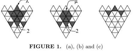
λ µ
[image:10.595.195.417.229.314.2]2 2
FIGURE 1. (a), (b) and (c)
For a non-trivial example, consider SL3 withp= 5, and a weight
λ in an alcove just above the lowest p2-alcove (as shown in Figure 1(a)). Nowλlies in ε2(D), whereD is the upper alcove in the set of
p-restricted weights. The decomposition diagram associated to Dis just Dand C1, each with multiplicity one. Thus for the p-alcove F containingλ, (and anyp-facet E) we have
cF E =dF E−dDC1cJ E =dF E−cJ E =dF E −dJ E
where J is the image of F in ε2(C1) under Wp2. For λ in F as
above, the p-alcove J is that containing µ in Figure 1(b). The de-composition diagrams for F and J are given in Figures 1(a) and (b) respectively, and so the virtual decomposition diagram associated to
F is that given in Figure 1(c). (All multiplicities are 1 unless other-wise indicated.) The virtual composition factors associated toλare just those weights inWp.λ lying in this final diagram.
Returning to our definitions, we next associate to eachpi+1-restricted weight λ a set of i-virtual composition factors (with multiplicities). When i = 1 these will just be the virtual composition factors de-fined above. Regard the pi-facets as p-facets by scaling. Then the pi-facet ε
i(F) containing λ corresponds to the p-facet F in the set
decomposition diagram. By scaling, we obtain a corresponding set of pi-facets with multiplicities. This is the i-virtual decomposition
diagram associated to εi(F), and the i-virtual composition factors
associated to λ are just those weights in Wpi.λ that lie in these pi-facets. We shall denote the corresponding multiplicity of such a
weight µby ci λµ.
Finally, we shall associate a set ofi-virtual composition factors to an arbitrary dominant weight λ. Any such weight can be uniquely written in the form λ = λ′+pi+1λ′′ with λ′ ∈ X
i+1(T). Now the
i-virtual composition factors associated to λ are just those weights of the form µ = µ′+pi+1λ′′ where µ′ runs over the set of i-virtual composition factors ofλ′, and ci
λµ=ciλ′µ′.
We will show that, for p ≥h, the following algorithm completely determines the decomposition numbers for a given Weyl module ∆(λ).
Algorithm 2.1.
(1) Let i be maximal such that λ does not lie in C¯i and let cf(λ, i+
1) ={λ}. (Thus λlies in the set of pi+1-restricted weights.) (2) If i= 0 then we are done, otherwise continue with step (3). (3) For each weightµ incf(λ, i+ 1)(and keeping track of multiplici-ties) determine the set of i-virtual composition factors associated to
µ.
(4) Let cf(λ, i) be the disjoint union of all the sets of virtual compo-sition factors (with multiplicities) obtained during step (3).
(5) Seti=i−1 and repeat from step (2).
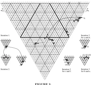
To illustrate the above algorithm we shall consider an example for SL3. Let p = 5 and consider the Weyl module ∆(181,0,0) for GL3 (where we use the usual partition labelling for polynomial dominant weights). This Weyl module is just the contravariant dual of a sym-metric power of the natural module, and so its composition factors can be calculated using the results in [8].
ω ω
d b
a c
e
f
(i) (ii)
(i) (ii)
(iii)
(i)(ii)(iii)
1 2
λ
Iteration 3 Iteration 3 for a and d. Iteration 3
for c and f. for b and e. Iteration 2.
[image:12.595.160.459.98.376.2]Iteration 1.
FIGURE 2.
the various virtual decomposition diagrams that arise during each it-eration of the algorithm. For future reference we have labelled the composition factors that arise; for example, λ corresponds to the labeld(i).
We begin by considering thep3-facets. After scaling, the p3-facet containingλcorresponds to the upper shadedp-alcove shown in Iter-ation 1. Thus the first iterIter-ation of the algorithm producesλand the element ofWp3.λlying just above the lowest p3-alcove (indicated by
a solid arrow). After the second iteration, the virtual decomposition diagrams given in Iteration 2 arise, and after scaling (and transla-tion for those associated toλ, since this is not ap3-restricted weight) these give weights in the alcoves indicated by dotted arrows. The final iteration uses the virtual decomposition diagrams shown in It-eration 3 to produce the set of shadedp-alcoves shown in the central diagram.
Theorem 2.2. Suppose that p ≥ h. Given a dominant weight λ,
the set of composition factors of ∆(λ) (counted with multiplicities) is precisely the set cf(λ,1) obtained from Algorithm 2.1.
Proof. First suppose thatλ∈X2(T). We will show that the sum of the characters of the virtual composition factors obtained from the algorithm isχ(λ), as required. We first note that ifλ∈C2, then the set of virtual composition factors associated toλis precisely the full set of composition factors of ∆(λ) (by our earlier remarks), and hence the result is immediate.
If λ∈X2(T) does not lie in C2 then as noted at the start of the section we must have λ∈ C3. Thus there are two iterations when the algorithm is applied to λ, and the set cf(λ,2) is just the set of composition factors arising from the p2-decomposition diagram. After the second iteration the multiplicity of µin cf(λ,1) is just
X
τ
dHIcτ µ=cλµ+
X
τ <λ
dHIcτ µ
where λ ∈ε2(H), τ ∈ Wp2.λ, and τ ∈ ε2(I). Comparing this with
(2), we see that this equalsdλµ as required.
Now suppose that λ is a pi+1-restricted weight with λ /∈C
i. We
set j =i−1 ifλ∈ Xi(T), and j =i otherwise. The first iteration
of our algorithm begins at level i, and cf(λ, i+ 1) ={λ}. We claim that, by Steinberg’s tensor product theorem, it is enough to show that
χ(λ) = X
µ∈cf(λ,j)
ch(L(µ′′)Fj
χ(µ′) + X
τ <µ′
ajµ′τχ(τ)
(3)
whereµ=µ′+pjµ′′and theaj
µ′τare defined in the following manner.
ForE andF p-facets in X1(T), we definea1F E by choosingλ∈F
and solving
chL(λ) = X
E≤F
a1F Eχ(µE)
where µE = (WP.λ)∩E. For weights µ′ ∈εi(F) and τ ∈ εi(E) in Xi(T), we define
aiµ′τ =
a1
F E if τ ∈Wpi.µ′
For the claim, note that for eachµon the right-hand side of (3) we have by our choice ofjthatµ′< λ. Thus by induction our algorithm gives the character ofχ(µ′) (and ofχ(τ) for allτ < µ′), but possibly starting at levelj. The effect of starting at levelj−1, as is the case when calculating for µ ∈ cf(λ, j), is to lose the elements descended from those elements of cf(µ, j) not equal to µ. After scaling, it can be seen that this corresponds to calculating decomposition numbers for the simple module in the correspondingp-alcove inX2(T) rather than of the Weyl module. Hence by the induction hypotheses and the definition of the ajµ′τ, it is enough to show (3).
Let chL(µ′′) =P
νmµ′′νe(ν). Then we wish to show that
P
µ
chL(µ′′)Fj P
τ≤µ′a j µ′τχ(τ)
=P
µ
P
νmµ′′νe(pjν)
P
τ≤µ′a j µ′τχ(τ)
=P
µ
P
νmµ′′ν
P
τ≤µ′a j
µ′τχ(τ +pjν)
=P
µ
P
νmµ′′ν
P
τ≤µ′a j
µ′τ(−1)l(wτ ν)χ(wτ ν(τ +pjν))
is equal to χ(λ) (where we write wτ ν forwτ+piν for brevity). This
expression is of the form
χ(λ) +X
θ<λ
fλθχ(θ)
for some coefficients fλθ (where all the weightsθ are dominant).
Now when j = 1 all these coefficients are zero by the calculation above, and the linear independence of the characters of Weyl mod-ules. But in general thefλθ depend only on thepjν, reflections about
the boundaries of the dominant region, and the combinatorics ofpj
-facets regarded as p-facets. Thus, after fixing an appropriate power of the Frobenius morphism, these coefficients depend only on the combinatorics of the pj-facets regarded as p-facets and the weights
of the L(µ′′). As for j = 1 all the fλθ are zero, the same must be
true for allj by scaling.
There is another recursive formula which can be used for deter-mining the composition factors of Weyl modules, due to Jantzen [13, 3.1 Satz]. For any weight λ∈X(T) we have
χ(λ) = X
µ′′∈X(T)
X
µ′∈Xr(T)
[ ˆZr(λ) : ˆLr(prµ′′+µ′)]χ(µ′′)F
r
where the ˆZr(λ) are certain coinduced modules for the Jantzen
sub-groupGrT ofG, and the ˆLr(λ) are the corresponding simple modules
(see [14, II Chapter 9] for details). Suitably far away from the walls of the dominant region, all the weights in this sum are dominant, and the equality corresponds to a filtration ofH0(λ) with factors of the formL(µ′)⊗H0(µ′′)Fr
(see [14, II 9.11 Proposition]). However, near the boundary of the dominant region, the µ′′ will not all be dominant, and although (4) can be modified using Lemma 1.2, the coefficients will now no longer all be positive.
Although the virtual composition factors associated to a single weight µ arising during Algorithm 2.1 may also (in principle) have negative multiplicities, we have
Lemma 2.3. For any dominant weight λ, the multiplicities of the
elements ofcf(λ, i)obtained after each iteration of Algorithm 2.1 are all positive.
Proof. Suppose there is someλfor which the lemma fails, and let
ibe as in Algorithm 2.1. Then there exists somej≤isuch that the setF of j-virtual composition factors obtained when consideringpj
-facets includes some negative multiplicities. Choseλ′such that it lies in thep-facet corresponding to the pi−j+1-facet containingλ(under scaling). Then the set of composition factors of H0(λ′) obtained using the algorithm will correspond (under scaling) to those in F, and have the same multiplicities. But these multiplicities are all positive, which gives the desired contradiction.
For there to be any possibility of obtaining a filtration of H0(λ) associated to our algorithm, it is clearly necessary that all the virtual composition multiplicities associated to a given weight are positive. We shall return to this question in Section 4. First however we shall exploit the easy invertibility of our algorithm.
3. RINGEL DUALITY AND REPRESENTATIONS OF THE SYMMETRIC GROUP
In this section we restrict our attention to the case where G is the general linear group GLn. Although not itself semisimple, its
representation theory can be easily deduced from that of SLn, and so
Schur algebras S =S(n, d), and in [10] Erdmann showed how their representation theory can be related to that of the symmetric group Σd by Ringel duality. We shall very briefly review this relationship
(details and further references can be found in [10]), and show how the invertibility of Algorithm 2.1 allows us to deduce certain results concerning representations of the symmetric group. Throughout this section we shall assume thatp > n.
The category ofS(n, d)-modules is naturally equivalent to the cat-egory of SLn-modules all of whose composition factors L(λ) satisfy
λ= P
iaiωi with Piiai = d−jn for some j ≥0. As S(n, d) is a
quasi-hereditary algebra, there exists a certain characteristic module
T for S, and we call the endomorphism algebra S′ = End
S(T) the
Ringel dual ofS. In fact (up to Morita equivalence) we can identify
S′ precisely:
Theorem 3.1. Suppose thatp > n. Then the Ringel dual ofS(n, d)
is Morita equivalent to a certain (known) quotient of kΣd, the group
algebra of the symmetric group on dsymbols.
Proof. This is a special case of the first part of [10, Theorem 4.4].
Let Λ+(n, d) be the set of n-part partitions of d. To each λ ∈
Λ+(n, d), we can associate a corresponding permutation moduleMλ
forkΣd, and certain explicitly defined submodulesSλ of Mλ, called
Specht modules. The indecomposable direct summands of Mλ are
called Young modules, and we defineYλ to be the unique such
sum-mand ofMλ containing Sλ.
It is shown in [6, (2.6)] that Young modules have a Specht module filtration, and we shall denote the multiplicity of Sµ in some such
filtration of Yλ by (Yλ : Sµ). It is easy to see (confer [20, 4.10
Corollary]) that ifλhas at mostrnon-zero parts, so also mustµfor any Sµ arising in such a filtration ofYλ. Indeed, by general results
on Ringel duals and the explicit identifications made in [10], we have
Proposition 3.2. Suppose that p > n. Then for allλ, µ∈Λ+(n, d)
we have
(Yλ:Sµ) = [∆(µ) :L(λ)].
Thus to determine the Specht modules arising in a given Young module Yλ for kΣ
d, it is enough to determine all Weyl modules
containing the simple module L(λ) for SLn with highest weight in
a certain bounded set of weights. Here n can be taken to be the number of non-zero parts of λ. The advantage of our algorithm for computing decomposition numbers is that it can easily be run in reverse. Starting with a given weightλand the initial data on Weyl modules corresponding to p2-restricted weights, it is easy to deter-mine those weights (with multiplicities) which give rise toλafter one iteration of Algorithm 2.1. Iterate this procedure by determining for each weight obtained at theith stage a corresponding set (with mul-tiplicities) of new weights in a similar way (by regardingpi-facets as p-facets). Thus (ash=n) we obtain
Proposition 3.3. Suppose thatp > n. Given a weightλ∈Λ+(n, d),
we can invert Algorithm 2.1 to give an algorithm for determining (Yλ :Sµ) for all µ∈Λ+(n, d), from the decomposition numbers for Weyl modules for SLn withp2-restricted weights.
4. LIFTING FROM THE QUANTUM GROUP
Although they arise naturally in the algorithm of Section 2, it is not yet clear that the sets of virtual composition factors have any representation-theoretic interpretation. In particular, it is not even clear that they have non-negative multiplicities. In this section we shall realize them as the sets of composition factors associated with
G-modules obtained by lifting from a corresponding quantum group — at least when p is large enough for the Lusztig conjecture to hold. We then discuss a possible connection with a long-standing conjecture of Humphreys on the structure of Weyl modules.
The modules we require arise in the work of Lin [16], and are generalisations of certain modules considered by Lusztig. The con-structions in this section are based on [16, Section 2], to which we refer the reader for further details.
We begin by defining the various quantum algebras that we re-quire. Let Uq be the quantised enveloping algebra over C(q)
Lusztig [19] has constructed a certain A-form UA of Uq. For ξ a
fixed primitive pr-th root of unity, C becomes anA-algebra via the
homomorphism taking q to ξ. We denote by Uξ the corresponding
algebraC⊗AUA.
Setting Br to be the localisation of Z[ξ] at the ideal (ξ−1), we
have that Br is a discrete valuation ring, and UBr = Br⊗AUA is
a Br-form inside Uξ. Finally, for k an algebraically closed field of
characteristic p, the natural homomorphism A → k taking q to 1 factors through the homomorphismB →ktakingξ to 1. We obtain an isomorphism ofk-algebras
Uk:=k⊗AUA =∼k⊗BrUBr.
We next wish to define various modules for each of these algebras, following Lusztig [17, 18, 19]. For each dominant weightλthere ex-ists a unique finite-dimensional irreducibleUq-moduleLq(λ) of type 1 with highest weight λ. If we fix some vector vλ generating this
module, then LA(λ) = UAvλ is a UA-invariant A-lattice in Lq(λ).
We set ∆pr(λ) = C⊗A LA(λ), the quantum Weyl module for Uξ.
This has a unique simple quotient, which we denote byLpr(λ). We
denote the image of our generating vectorvλ in this quotient by ¯vλ.
Now LBr(λ) = UBr¯vλ is a Br-lattice in Lpr(λ), and so Lpr(λ) = k⊗Br LBr(λ) is a Uk-module. Indeed, Lusztig has shown that this
is even a (rational) G-module. The Weyl module for G can also be constructed usingUq; we have
∆(λ)∼=k⊗ALA(λ)∼=k⊗Br∆Br(λ)
where ∆Br(λ) =UBrvλ is aBr-lattice inside ∆pr(λ).
Our construction gives thatLpr(λ) is a quotient of ∆(λ), and we
wish to understand the structure of these modules. By [16, Theorem 2.7], we have that
Lpr(λ)∼=Lpr(λ′)⊗∆(λ′′)F r
where λ = λ′ +prλ′′ with λ′ ∈ X
r(T), and F denotes the usual
Frobenius morphism. Thus we first need to understand the structure of Lpr(λ) for all pr-restricted weights.
λis suitably far away from anypi-walls for certaini; see [16, pg 286] for the precise definition.) For arbitrary dominant weights λand µ
we have
[∆(λ) :L(µ)] =X
ν
[∆pr(λ) :Lpr(ν)][Lpr(ν) :L(µ)]. (5)
It is this identity that will allow us to relate our algorithm to the decomposition patterns of theLpr(λ).
For the rest of this section, we shall assume that Lusztig’s conjec-ture (for algebraic groups) holds for our choice ofGand p, and that
p≥2h−2. For fixedGthis is known to be the case if we take p to be sufficiently large by the results in [1].
A dominant weightλsatisfies the Jantzen condition ifhλ+ρ, αˇi ≤
p(p+ 2−h) for all α∈R+. For suchλwe have
[∆p(λ) :Lp(µ)] = [∆(λ) :L(µ)]
and we see by induction using (5) thatLp(λ)∼=L(λ) is irreducible.
More generally we shall say that a dominant weightλsatisfies the
ith Jantzen condition if
hλ+ρ, αˇi ≤pi(p+ 2−h)
for all α ∈ R+, and denote the set of such λ by Ji(T). Note that λsatisfies the Jantzen condition if and only ifεi(λ) satisfies theith
Jantzen condition. Forλ∈Ji(T) we have
[∆pi(λ) :Lpi(µ)] =
dF E if µ∈Wpi.λ
0 otherwise (6)
whereλ∈εi(F) andµ∈εi(E). Asp≥2h−2 we have thatXi(T)⊆ Ji(T), and hence for p2-restricted weights, thep2-decomposition
di-agrams defined in Section 2 are just the decomposition didi-agrams for the corresponding quantum group at ap2 root of unity.
We next define some more sets of weights associated to Algorithm 2.1. It will be convenient to set cf(λ, i) = {λ} whenever λ ∈ C¯i,
extending our earlier notation. Given a weight λ and an integer
i we have, by construction, λ∈ cf(λ, i), with multiplicity one, and all other weights µ∈cf(λ, i) satisfy µ < λ. We define Desc(λ, i) by induction onλvia
cf(λ,1) =
.
[
µ∈cf(λ,i) Desc(µ, i)
where as usual we run over elements of the index set counted with multiplicities.
As an example, consider the weight denoted λ in Figure 2. For
i ≥ 4 we have Desc(λ, i) = cf(λ,1), the set of composition factors of ∆(λ). The set Desc(λ,3) is precisely the set of those weights with labels of the form d(–), e(–), or f(–), while Desc(λ,2) ={λ=
d(i), d(ii)} and Desc(λ,1) ={λ}. The main result of this section is
Theorem 4.1. Suppose that p ≥ 2h−2 is such that the Lusztig
conjecture is satisfied forG. Ifλ∈Ji(T) then the set of composition
factors, with multiplicities, ofLpi(λ) equals Desc(λ, i).
Proof. We proceed by induction onλ. Ifλlies in ¯Ci, then cf(λ, i) =
{λ} and hence Desc(λ, i) = cf(λ,1). But in this case, as [∆pi(λ) : Lpi(µ)] = δλµ we see from (5) that Lpi(λ) = ∆(λ), and so we are
done by Theorem 2.2.
Now suppose that λ /∈ C¯i. As Ji(T) ⊆ Ci+1, we see that Algo-rithm 2.1 begins at leveli, and cf(λ, i+ 1) ={λ}. After scaling byεi,
the pi-facet containing λ corresponds to some p-facet F in C
2. By our remarks before Algorithm 2.1, this implies that the virtual de-composition diagram associated toF is just the usual decomposition diagram for F. Hence after scaling by εi we see that
ciλµ =
dF E if µ∈Wpi.λ
0 otherwise
where λ ∈ εi(F) and µ ∈ εi(E). But by (6) this equals [∆pi(λ) : Lpi(µ)]. Hence we have by Theorem 2.2 that the composition factors
of ∆(λ) are given by cf(λ,1), where
cf(λ,1) =
.
[
whereµruns over the set of dominant weights. By induction, we see by comparing with (5) that Desc(λ, i) is precisely the set of compo-sition factors ofLpi(λ), as required.
Recall that forp≥2h−2 we have Xi(T)⊂Ji(T). Thus for
suit-ably large p, our algorithm gives a means of calculating the compo-sition factors ofLpi(λ) for allpi-restricted weights, given the
decom-position numbers for ∆(µ) forp2-restricted weightsµ. In particular, for anyp2-restricted weightλwe have that Desc(λ,2) is just the set of virtual composition factors associated toλ, and hence obtain
Corollary 4.2. Suppose that p≥2h−2 is such that the Lusztig
conjecture is satisfied forG. Then for anyp2-restricted weightλ, the virtual decomposition numbers cλµ are all non-negative.
Recall from Section 1 that for any weightλwe may define modules
Hj(λ) by considering the right derived functors of indG
B. In [11],
Humphreys has conjectured that any Weyl module ∆(λ) should have a filtration with quotients of the form Hj(µ)⊗L(ν)Fi
, whereµ is
W-conjugate to a weight inXi(T) andν is dominant. On the level
of characters, this would imply that ∆(λ) has a filtration where each quotient has composition factors clustered around a certain translate of Xi(T) (related to the weight ν defined above).
Now suppose that there exists a filtration of ∆(λ) associated to the ith level in Algorithm 2.1; that is, a filtration whose successive quotients have sets of composition factors of the form Desc(µ, i) for elements µ ∈ cf(λ, i). On the level of characters, this would imply that ∆(λ) has a filtration where each quotient has composition fac-tors clustered around a certain pi-alcove (related to the weight µ).
In proving (5), Lin constructs an associated filtration of the Weyl module, which by Theorem 4.1 is compatible with the first iteration of Algorithm 2.1.
Theorem 4.3. Suppose that λ is a dominant weight for SL3 such
that all composition factors of Zˆ1(λ)lie in the same p2-alcove. Then there is a filtration of ∆(λ) corresponding to the final iteration of Algorithm 2.1.
Proof. This is an easy consequence of a theorem of K¨ uhne-Hausmann [15, Kapitel VI, Satz 2].
More generally, K¨uhne-Haussman has calculated the submodule structure of all Weyl modules for SL3 which are multiplicity-free. For the examples given in [15, pages 174-6] — which do not satisfy the hypotheses of Theorem 4.3 — it is easy to verify that there is still a filtration associated to our algorithm.
If we assume that Humphreys’ conjecture holds, the above remarks gives some evidence that there may be a refinement of his filtration associated to the corresponding level of Algorithm 2.1. In the next section we shall consider further evidence for the existence of such a filtration.
5. A SOCLE SERIES FOR CERTAIN INDUCED MODULES
In this section we shall show how the facet combinatorics intro-duced in Section 2 can be used to give a new description of certain results of Doty in [8]. In particular we shall give a filtration (and for weights in alcoves a description of the socle series) of symmetric powers of the natural module for SL2 and SL3. These are isomorphic to induced modules of the formH0(dω
1), which in turn are just the contravariant duals of the corresponding Weyl modules (and have the same composition factors). Thus this filtration will provide an interpretation in terms of module structure of the character-theoretic result in Section 2.
These results could also be deduced from [3] for SL2, and [15, Kapitel VI, Satz 1] for SL3. However, we prefer to consider the methods of Doty as these are both simpler and more accessible to generalisation to groups of higher rank.
We begin by recalling the combinatorial framework outlined in [8]. LetSd(V) denote thedth symmetric power of the natural represen-tation V of GLn. We write d= PMi≥0dipi with 0 ≤ di ≤ p−1 for
write bi = Pj≥0bijpi with 0 ≤ bij ≤ p−1 for all i and j. Then
we can associate to each monomial xb
an M-tuple of non-negative integers (c1(b), . . . , cM(b)), where the elementsck(b) are defined by
the equations
X
i≥0
X
j<k
bijpi=ck(b)pk+
X
j<k djpj.
An equivalent set of defining equations are given by
X
i≥0
bik =dk+pck+1−ck. (7)
We let C(d) be the set of M-tuples arising from some xb
∈Sd(V).
This set can be given a lattice structure by settingc≤c′ if and only if ck≤c′k for all k. Then the main result in [8] is
Theorem 5.1. There is a lattice isomorphism between the lattice of
order closed subsets ofC(d)and theG-submodules ofSd(V)(ordered
by inclusion). In particular, the composition factors ofSd(V)are in
one-to-one correspondence with the elements of C(d).
Further, by considering (7), we can determine explicitly the highest weight vector of the composition factor corresponding tocas follows. Let xb
be the highest weight vector corresponding to c. Then b is given by the set of equations
bik= max{min{dk+p(ck+1+ 1−i)−ck+i−1, p−1},0} (8)
where thedkand bik are as defined above. Thus, given the set C(d)
corresponding to d, we can determine the composition factors of
Sd(V). The final result from [8] that we shall need is the following
criterion for recognising elements of C(d).
Lemma 5.2. An M-tuple c of non-negative integers is an element
of C(d) if and only if it satisfies the equations
0≤ck≤
X
j≥k djpj−k
and
for allk, where we set cj = 0 for allj ≤0 and j > M.
We begin by analysing the structure of the lattice C(d). First we note that by induction (using Lemma 5.2) it is clear that we must have 0 ≤ ck ≤ n−1 for each k. Given c ∈ C(d), we set
|c| =P
i≥0ci. We shall say that such an element c lies in the jth
socle layer Socj(C(d)) ofC(d) if the longest chain of elements strictly
belowc is of length j−1.
Lemma 5.3. An element c∈C(d) lies in thejth socle layer if and
only if|c|=j.
Proof. Any chain of elements strictly below c must have length at most |c|, and so it is enough to show that a chain of this length in fact exists. For this, it will be enough to show that for eachc6=0
there exists some c′ < c in C(d) such that for some k0 we have
c′k0 =ck0 −1, andc ′
i =ci for alli6=k0.
We first claim that if c 6= 0 then there exists some k such that
0 ≤dk+pck+1−ck < n(p−1) and ck 6= 0. For otherwise take k1
minimal such thatck0 6= 0. Then we must havedk1+pck1+1−ck1 =
n(p−1) ≥ p, and hence that ck1+1 > 0. In a similar manner we
deduce that ck > 0 for all k ≥k1 (and that for all such k we must havedk+pck+1−ck=n(p−1)). But this contradicts the condition
thatcM+1= 0, and so the claim follows.
Takingk0 to be minimal satisfying the above hypotheses, it is now an easy exercise using the inequalities in Lemma 5.2 to verify that the element c′ defined above is inC(d) as required.
Most of the rest of this section will be devoted to proving
Proposition 5.4. For GL2 and GL3, the modules Sd(V) have
fil-trations corresponding to the virtual decomposition factors obtained at any given stage in Algorithm 2.1. Moreover, for weights in the interior of alcoves, the socle series for Sd(V) can be constructed in
the course of implementing the algorithm.
Proof. To each composition factorL(λ) we have associated a carry patternc(λ). We shall show that the iteration of Algorithm 2.1 cor-responding topi-facets changes the value only of the firstielements
obtained at this stage from a given weight corresponds to a differ-ent value of ci. In fact, for weights in the interior of an alcove we
shall show that at this stage the firstielements of any carry pattern obtained so far are all equal. By Lemma 5.3, we shall thus obtain complete information on the socle series of the symmetric powers corresponding to weights in the interior of an alcove.
We begin with an easy example to illustrate this result for SL2. (We postpone analysis of the socle series for the SL3 example given in Figure 2 until later in this section.) Let p = 3 and d = 43. On applying Algorithm 2.1 we obtain the set of composition factors labelleda to f in Figure 3.
f db c e a
p -12 p -13 -1 p-1
FIGURE 3.
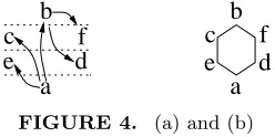
For SL2, the p2-restricted weights are precisely those in the upper closure of the lowestp2 alcove. Thus the virtual composition factors associated to a weight are just the ordinary composition factors of the corresponding Weyl module. This is simple for weights on walls or in the lowest p-alcove, and has two composition factors corresponding to the highest weight and its reflection about thep-wall immediately below it for weights in the remaining p-alcoves. As in this case the various ci can only be 0 or 1, the corresponding socle series
predicted by our result will be as shown in Figure 4(a) (with the actual submodule lattice obtained using the results in [8] given in Figure 4(b)).
a b
f d c e a
[image:25.595.244.368.505.567.2]b f d c e
FIGURE 4. (a) and (b)
the required form. For this we need to know the relative positions of the virtual composition factors for certainp2-restricted weights. It is for this reason that we restrict ourselves to considering SL2and SL3, although we conjecture that the result should hold for SLn without
restriction onn.
In order to convert the results from [8] for GLninto a form
compat-ible with the facet geometry, we use the usual change of coordinates
λ= (λ1, . . . , λn)7−→λ¯ = (¯λ1, . . . ,λ¯n−1), where we set ¯λi=λi−λi+1. This now gives the coordinates of the corresponding SL-weight in terms of the basis of fundamental weights.
We begin by considering the SL2 case. Let b = (b1, b2) be the highest weight vector in some composition factor of Sd(V). By the
preceding remarks and Theorem 2.2 this is either (d,0) or ¯b is a reflection of some ¯b′ about a pi-wall for some weight b′ generated at an earlier stage in the algorithm (where we takei to be maximal with this property). Let the corresponding elements of C(d) be c
and c′ respectively.
It will be enough to show that ck = 1−c′k when 1 ≤ k ≤ i and ck =c′k otherwise. Suppose that ¯b′ = api−1 +b with 0 < b < pi
and a 6≡ 0 mod p. Then it will suffice to show that the weight ¯x
corresponding to the desired value of ¯csatisfies ¯x+ ¯b′= 2api−2 (as
then ¯x must equal ¯b). By considering the various possible values of
b′ik arising from (8) we see that
¯b′
k=b′1k−b′2k =
dk if (ck, ck+1) = (0,0)
p−dk−2 if (ck, ck+1) = (0,1)
dk−1 if (ck, ck+1) = (1,0)
p−1−dk if (ck, ck+1) = (1,1).
(9)
Clearly, we must have{(c0, c1),(c′0, c′1)}={(0,0),(0,1)}, while for 1≤t≤i−1 we have{(ct, ct+1),(c′t, c′t+1)}={(0,0),(1,1)}. Further, by our inductive hypothesis we must have {(ci, ci+1),(c′i, c′i+1)} =
{(0,1),(1,1)} or {(1,0),(0,0)}. Using (9) it is now easy to see that
X
k
(¯b′k+ ¯xk)pk =p−2 + i−1
X
t=1
(p−1)pt+ (2a−1)pi= 2api−2
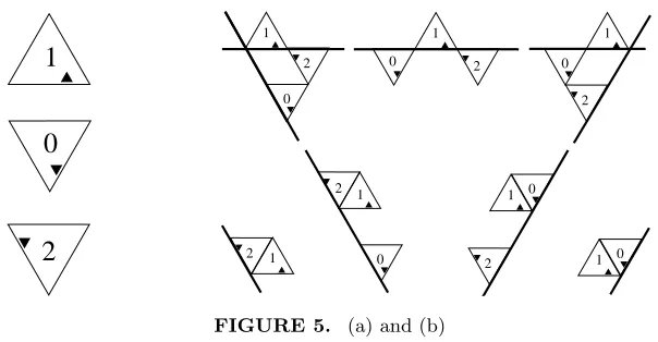
The proof for SL3 proceeds in a similar manner. We shall first consider the case where the initial weight lies in the interior of an alcove, and show that when consideringpt-alcoves, the set of virtual
composition factors associated to a given weight contains at most one of each of the three types of alcove shown in Figure 5(a). Further, we show that the image of the given weight underWpt in each of these
alcoves corresponds to the carry pattern whose first t elements are equal to the integer labelling that diagram, and that the remaining elements of the carry pattern are fixed for these alcoves.
2
1
0
1
2
0
1
2 0
1
0
2
2 1
0 2
0 1
[image:27.595.154.456.232.389.2]2 1 1 0
FIGURE 5. (a) and (b)
Using (4), and the known decomposition numbers for the ˆZ1(λ) for SL3 [12], it is easy to show that the various possible patterns of virtual composition factors associated to weights outside the lowest
p-alcove are as shown in Figure 5(b).
It just remains to consider the various possible cases, calculate the weights corresponding to the predicted carry patterns, and verify that the differences between them correspond to the relative posi-tions of the various weights shown in each case. This is a routine (if lengthy) exercise using the expression for thebik given in (8).
If the initial weight does not lie in an alcove, then the strong ver-sion of the inductive hypothesis (asserting the precise form of the corresponding carry patterns) is no longer satisfied. However by similar arguments one shows that at every stage the virtual compo-sition factors correspond to distinct values of an appropriatect, and
that the ct′ (for t′ > t) remain constant. This completes the proof
000 020 110 120 210
220 211 221
100 121
010 001
021
101 011 111 b(iii)
f(i) c(ii)
f(ii) c(iii)
f(iii) b(i) a(ii)
a(i) e(i)
b(ii) e(iii)
e(ii)
d(ii)
[image:28.595.168.434.102.236.2]d(i) c(i)
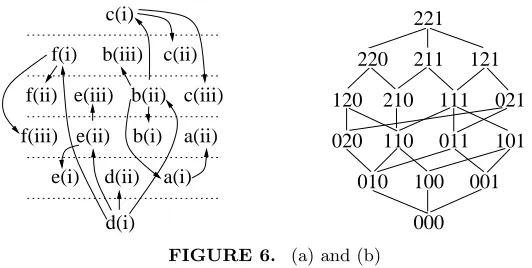
FIGURE 6. (a) and (b)
To illustrate the SL3 case, we return to the example considered in Figure 2. In Figure 6(a) we give the socle series constructed in the proof of Proposition 5.4, while in Figure 6(b) we give the corre-sponding submodule lattice calculated using [8]. The labels on the left are those used in Figure 2, while on the right the corresponding elements of C(d) are given.
6. THE QUANTUM MIXED CASE
To conclude, we consider the quantum general linear group q -GL(n, k) defined by Dipper and Donkin [5], in the case when q is a primitive lth root of unity and k has characteristic p > 0. Algo-rithm 2.1 can easily be modified to give a corresponding algoAlgo-rithm in this context, by replacing pi-facets by lpi−1-facets, and taking as the initial dataset the decomposition numbers for all lp-restricted weights.
Now the same arguments as in Sections 1 and 2 can be applied to show that this gives the composition factors of the quantum Weyl module corresponding toλ. For the results on the geometry of facets it is sufficient to require that bothl and p are at least as big as the Coxeter number, which in this case isn. The general theory reviewed in Section 1 is given in the quantum case in [7] and [4].
symmet-ric powers used in Section 5 have been generalised to the quantum setting in [21].
ACKNOWLEDGMENTS
I would like to thank Paul Martin and Alison Parker for several useful dis-cussions, and Steen Ryom-Hansen for sharing certain tilting module calculations that helped in part to motivate this project. I am also very grateful to Jens Jantzen for bringing the work of Lin to my attention.
REFERENCES
1. H. H. Andersen, J. C. Jantzen, and W. Soergel. Representations of quantum groups at a p-th root of unity and of semisimple groups in characteristicp: independence ofp. Ast´erisque, 220, 1994.
2. N. Bourbaki. Groupes et alg`ebres de Lie (Chapitres 4–6). Hermann, 1968.
3. R. Carter and E. Cline. The submodule structure of Weyl modules for groups of type A1. InProceedings of the Conference on Finite Groups (Park City, 1975), pages 303–311, 1976.
4. A. G. Cox. The blocks of theq-Schur algebra. J. Algebra, 207:306–325, 1998.
5. R. Dipper and S. Donkin. Quantum GLn. Proc. London Math. Soc. (3), 63:165–211, 1991.
6. S. Donkin. On Schur algebras and related algebras II. J. Algebra, 111:354–364, 1987.
7. S. Donkin. The q-Schur algebra, volume 253 of LMS Lecture Notes Series. Cambridge University Press, 1998.
8. S. Doty. Submodules of symmetric powers of the natural module for GLn. Contemp. Math., 88:185–191, 1989.
9. S. Doty and J. B. Sullivan. Filtration patterns for representations of algebraic groups and their Frobenius kernels. Math. Z., 195:391–407, 1987.
10. K. Erdmann. Symmetric groups and quasi-hereditary algebras. In V. Dlab and L. L. Scott, editors,Finite dimensional algebras and related topics, pages 123–161. Kluwer, 1994.
12. J. C. Jantzen. ¨Uber das Dekompositionsverhalten gewisser modularer Darstellungen halbeinfacher Gruppen und ihrer Lie-Algebren. J. Alge-bra, 49:441–469, 1977.
13. J. C. Jantzen. Darstellungen halbeinfacher Gruppen und ihrer Frobenius-Kerne. J. reine angew. Math., 317:157–199, 1980.
14. J. C. Jantzen. Representations of algebraic groups. Academic Press, 1987.
15. K. K¨uhne-Hausmann. Zur Untermodulstruktur der Weylmoduln f¨ur SL3. Bonner Math. Schriften, 162, 1985.
16. Z. Lin. Highest weight modules for algebraic groups arising from quan-tum groups. J. Algebra, 208:276–303, 1998.
17. G. Lusztig. Modular representations and quantum groups. InClassical groups and related topics, volume 82 ofContemporary Math., pages 59– 77. Amer. Math. Soc., 1989.
18. G. Lusztig. Finite-dimensional Hopf algebras arising from quantized universal enveloping algebras. J. Amer. Math. Soc., 3:257–296, 1990.
19. G. Lusztig. Quantum groups at roots of 1.Geom. Dedicata, 35:89–113, 1990.
20. A. Mathas.Iwahori-Hecke algebras and Schur algebras of the symmetric groups, volume 15 ofUniversity lecture series. American Mathematical Society, 1999.