DEVELOPMENT OF AN ADAPTIVE WINDOW OPENING ALGORITHM TO PREDICT THE THERMAL COMFORT, ENERGY USE AND OVERHEATING IN BUILDINGS
H.B. Rijal*1, P. Tuohy2, F. Nicol1, M.A. Humphreys1, A. Samuel2, J. Clarke2
1Oxford Institute for Sustainable Development, Oxford Brookes University, OX3 0BP, UK
2Energy Systems Research Unit, University of Strathclyde, Glasgow G1 1XJ, UK
ABSTRACT
This investigation of the window opening data from extensive field surveys in UK office
buildings demonstrates: 1) how people control the indoor environment by opening windows;
2) the cooling potential of opening windows; and 3) the use of an ‘adaptive algorithm’ for
predicting window opening behaviour for thermal simulation in ESP-r. It was found that
when the window was open the mean indoor and outdoor temperatures were higher than when
closed, but show that nonetheless there was a useful cooling effect from opening a window.
The adaptive algorithm for window opening behaviour was then used in thermal simulation
studies for some typical office designs. The thermal simulation results were in general
agreement with the findings of the field surveys. The adaptive algorithm is shown to provide
insights not available using non adaptive simulation methods and can assist in achieving more
comfortable, lower energy buildings while avoiding overheating.
KEYWORDS
Adaptive thermal comfort, Building control, window opening algorithm.
INTRODUCTION
Good building design is one of the important factors for energy saving; another is how
occupants control windows to achieve comfortable indoor conditions. Although adaptive
thermal comfort models are established (ASHRAE 2004, CIBSE 2006, CEN 2007), and
relationships between indoor and outdoor conditions and the use of building controls have
been described (e.g. Nicol 2001, Nicol and Humphreys 2004), there remains uncertainty in
how to design naturally ventilated buildings that achieve comfortable thermal conditions. It is
important to integrate into building design procedures occupant behaviour in relation to
windows as they are the most common thermal control device. When people feel too warm or
too cool they often open or close windows to alleviate their discomfort. This is not only
potentially useful for energy saving in summer, reducing the need for mechanical cooling, but
also provides a beneficial link with the outdoor environment. The basis of this occupant
behaviour is not yet fully understood, and so behaviour protocols for which there is little
empirical support have sometimes been employed (Rijal et al. 2007).
In the UK building regulations, domestic dwellings now require a summer overheating
calculation to be carried out using a standard methodology (BRE 2005), while the guidance
for non domestic dwellings for summer overheating has recently been revised with the issue
of CIBSE TM37 2006. The guidelines on how to achieve compliance, set static thresholds
and take no explicit account of outside daily or hourly temperature variations, or actual
building ventilation paths and their interaction with the external climate. Other guidelines for
building overheating performance do account for climate variations and permit dynamic
simulation but specify fixed values for the number or percentage of occupied hours allowed
Adaptive comfort temperatures are now a well established concept (Nicol and Humphreys
2007) in which indoor comfortable temperatures vary with the running mean outdoor
temperature. The adaptive behaviour applies to free running naturally ventilated buildings
where the occupants have opportunities for adapting by, for example, adjusting clothing,
posture, windows, blinds or fans. Adaptive comfort temperatures are now included in CIBSE
(2006) and ASHRAE (2004) guidelines and most recently the CEN standard EN15251
(Olesen 2007). To make studies of occupant adaptive comfort possible using dynamic
simulation at the building design stage, adaptive temperature algorithms must be implemented
into the program codes.
In an adaptive building, performance is dependent on how the building responds to internal
and external variations in climate and on how and when the occupants respond to these
variations (i.e. what adaptive actions they take and under what conditions they take them) and
on how these actions alter the building’s state. In order to model the performance of naturally
ventilated buildings it is essential to be able to model the occupant behaviour. Among the
most common adaptive actions in a naturally ventilated building is the adjustment of window
position.
Historically many window opening models have been put forward based on indoor or outdoor
temperature (Warren and Parkins 1984, Fritsch et al. 1990, Nicol et al. 1999, Raja et al. 2001,
Nicol and Humphreys 2004, Inkarojrit and Paliaga 2004, Yun and Steemers 2007, Herkel et
al. 2007). Fritsch et al. (1990) proposed a model based on Markow chains for random window
opening prediction. Pfafferott and Herkel (2007) used Monte-Carlo simulations to predict
user behaviour. Herkel et al. (2007) develop a window opening algorithm based on outdoor
Rijal et al. (2007) evolved the Humphreys window opening algorithm based on adaptive
comfort criteria in conjunction with indoor and outdoor temperatures and demonstrated its
application within the ESP-r simulation program. The combination of the adaptive comfort
temperature together with the modelling of comfort driven occupant adaptive behaviour was
shown to be important in achieving accurate representation of comfort and energy
performance in a naturally ventilated building. ESP-r was chosen as the simulation modelling
code for this work as its Open Source nature supports dissemination and adoption of the
methods in other software tools. ESP-r already offers several behavioural models such as the
Hunt model (Hunt 1979) for the switching of office lighting, the stochastic Lightswitch 2002
algorithm developed by Reinhart (2004) to predict dynamic personal response and control of
lights and blinds as well as Newsham et al.’s (1995) original Lightswitch model. Bourgois et
al. (2006) developed the SHOCC module to enable sub-hourly occupancy modelling and
coupling of behavioural algorithms such as Lightswitch 2002 across many ESP-r domains.
Anecdotally, an additional driver of window opening is air freshness, which may also be
modelled using ESP-r’s embedded contaminant modelling and CFD capabilities.
Naturally ventilated or hybrid ventilated buildings are common. The quantification of the
comfort and energy use performance of these buildings is however an area under
development. The importance of good understanding and good practice in this area is being
heightened by increasing outdoor temperatures and the increased focus on reductions in
building energy use within a number of countries. It is important to understand and model
correctly the behaviour of occupants in buildings and how this behaviour affects energy use
and comfort. It is similarly important to understand how a building’s design affects occupant
comfort, occupant behaviour and, ultimately, the energy used in the operation of the building.
This paper reviews the implementation of the EN15251 adaptive comfort criteria and the
application to an analysis of summer overheating for an office in the UK. The effect of
several building design options is then investigated and the use of the Humphreys adaptive
model compared to the use of proportional window opening above a static threshold
temperature for a number of building design options. Thus, the main objectives of this
research are (Rijal et al. 2007a, Tuohy et al. 2007):
• To understand how people use windows to control the indoor environment.
• To use an algorithm for window opening behaviour, derived from field data, for some
appropriate thermal simulations.
• To evaluate the cooling effect of window opening, by means of field investigations
and thermal simulation.
• To analyze the impact on summer overheating of window opening behaviour for a
variety of building design options.
• To compare the adaptive behavioural approach with non adaptive approaches.
THE DATABASE
This investigation uses data from extensive thermal comfort surveys in Oxford and Aberdeen
in the UK. Longitudinal (Abdnox-long) and transverse (Abdnox-trans) surveys were
conducted in 15 office buildings (7 naturally ventilated (NV) and 2 air conditioned (AC)
buildings in Oxford, 3 NV and 3 AC buildings in Aberdeen). The longitudinal surveys took
place between March 1996 and September 1997. Data loggers recording the room
temperature were placed in the working environment and the occupants were asked to record
in a brief questionnaire their thermal satisfaction and use of building controls. These
afternoon). 35,764 sets of responses were collected from 219 people. The transverse surveys
were conducted monthly during the period of the longitudinal surveys, researchers visiting
each building with thermal instruments logging air temperature, globe temperature and
humidity, backed by a questionnaire. On each visit, one set of responses was recorded from
each person. A total of 4,997 sets were collected from 890 people. Further details can be
found in Rijal et al. (2007).
EXPLORING THE WINDOW DATA
The proportion of windows open was very low in the AC buildings, there being few openable
windows, and so these buildings are excluded from further analysis. The proportion of
windows open in NV buildings was, as expected, lowest in winter, highest in summer and
intermediate in spring and autumn (Rijal et al. 2007).
Temperatures for windows open and closed
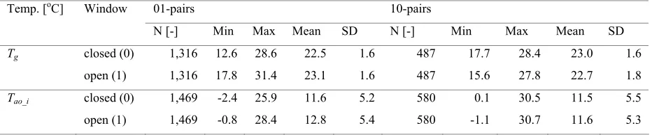
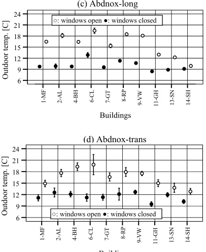
The values of globe temperature (Tg) and outdoor air temperature (Tao_i) for the windows open
and for windows closed cases are shown in Figure 1 and Table 1. The mean values of Tg and
Tao_i with windows open for all buildings of longitudinal survey are 23.4oC and 15.6oC
respectively. They are 1.2 K and 5.9 K respectively higher than with the windows closed. The
results are consistent with people opening windows in response to increases in the indoor
temperature, associated with raised outdoor temperatures. If the indoor temperature becomes
too high while the outdoor temperature is low (e.g. with high solar gain on sunny winter days)
the window will be opened, but generally only for a short period, because the room will
quickly cool down again.
Even though the methods of investigation and the number of samples are different in the two
surveys, the temperature associated with open windows is similar in both cases, as is that with
cases with the windows open and all case with windows closed is higher in Oxford than in
Aberdeen (11-GH, 13-SN and 14-SH). These regional differences might be attributable to the
difference in the climate between the two areas, which could also affect the occupants’
window opening behaviour.
Near Here: Figure 1 and Table 1.
Range of temperatures at which windows are open and closed
To show the lower (≤10%) and upper (≥90%) temperature bounds for windows open and
closed, the cumulative distributions of Tg and Tao_i are shown in the Figure 2. The results are
given in Table 2. The lower and upper bounds of Tg and Tao_i with windows open are higher
than with the window closed in both surveys. It is interesting that there is little temperature
difference between window open and closed at the lower and upper limit. The results show
that people open windows over a wide range of indoor and outdoor temperatures.
Near Here: Figure 2 and Table 2.
Effect of opening a window
In this analysis an open window is designated by ‘1’ and a closed window by ‘0’. To find
from the longitudinal data the effect of opening a window, pairs of responses when a closed
window was followed by an open window (01 pairs) were extracted within the same day from
the same person. Although the people had been requested to make records 4 times in a day,
some provided only 2 or 3. Consequently, some of the selected samples had 1 or 2 record
gaps between them, but most were separated by about 2 hours.
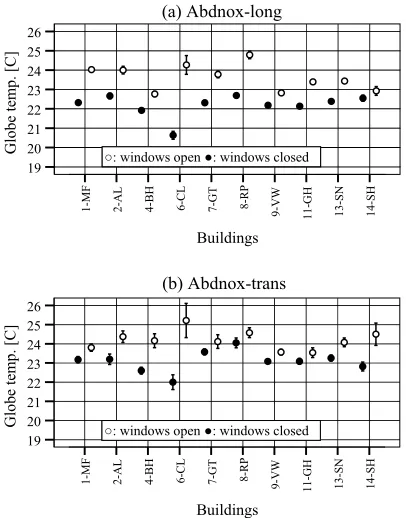
The number of paired samples is 1,316 for Tg. The mean Tg and Tao_i for the windows open is
higher than for the windows closed (Figure 3 (a), (b) and Table 3). As the value of the
outdoor temperature can not be influenced by the action of opening the window, the window
of opening the window was to limit any subsequent rise in room temperature that would have
occurred had the window remained closed, rather than to cool the room. As well as window
opening affecting the indoor temperature, there may also be an air movement or fresh air
advantage.
Near Here: Figure 3 and Table 3.
Effect of closing a window
To find the effect of closing a window, open-closed (10) pairs of responses were selected.
Again they were from records adjacent in time, within the same day, and from the same
person. The number of samples for this condition is small (n = 487 for Tg) because people
rarely closed windows in the offices once they were open, probably because during the day
both indoor and outdoor temperatures were generally rising. When the windows were closed,
in most of the buildings Tg increased and Tao_i decreased (Figure 3 (c), (d) and Table 3). It
seems that people were likely to close windows when the outdoor temperature was falling.
The results suggest that windows are closed to effect an increase in the indoor temperature, or
to limit its fall, by shutting off the effect of falling outdoor temperatures.
The cooling effect of open windows
To investigate the cooling effect of having the windows open, the globe temperatures for
weekdays and weekends are compared. The sequences Friday to Monday inclusive, in
August, September and May-June, were chosen. In each period, the outdoor temperature
profiles were similar and the heating was off. For the analysis 15 people were selected from 5
buildings in Oxford. The analysis is for office hours (9:00 to 17:00). It is assumed that all
windows were closed during the weekend. During weekdays the proportion of windows open
was always high in these periods, so the windows were taken to be open. The globe
The internal heat gains (from occupancy, lights and equipment) are small at the weekend, and
the indoor air movement is low. There are no air movement records from the Aberdeen and
Oxford data, but in the SCATs data (McCartney and Nicol 2002), a European project of
similar design, the mean air velocity with windows open in NV buildings was 0.06 m/s higher
than with the windows closed (P<0.001). This difference can be shown to be equivalent to a
reduction of about 0.6 K (Humphreys and Nicol 1995) in the globe temperature, and this
amount is subtracted from the globe temperatures in the weekdays. The mean temperature rise
due to the internal heat gain is estimated from the difference between the adaptive windows
open algorithm and windows closed of 13:30 to 17:30 (Rijal et al. 2007). This is equivalent to
1.7 K and this amount is added to the globe temperatures at the weekend. This process gives
an indication of what the indoor temperature would have been during weekdays had the
windows not been opened. The results are shown in Figures 4 and 5.
The temperature difference between the windows open and closed cases is small in a
heavyweight building (9-VW in Figure 4). Overall, the mean globe temperature when
windows were open (weekday) was 2.2 K lower than when the windows were closed
(weekend). The results show that if occupants had not opened windows during weekdays, the
indoor temperature would have continued to rise. Thus, opening windows had a significant
cooling effect. This can explain the previous finding that the comfort temperature with use of
controls is higher than without use of controls (Brager et al. 2004 and Robinson and Haldi
2007).
A further illustration might be helpful. Figure 6 compares Tg for the windows open (Fridays
and Mondays) and closed (Saturdays and Sundays) cases for each person. Each point
represents one person for the selected days during that month. The temperatures for windows
cooler side of the figure. This comparison of Tg for windows open and closed clearly shows
the cooling potential of open windows.
Near Here: Figures 4, 5 & 6
Development of window opening algorithm
A previous paper described the construction of a practical algorithm for incorporation into
ESP-r (Rijal et al. 2007). Logistic multiple regression analysis was used to construct an
equation to predict the probability of windows being opened from a knowledge of the indoor
and outdoor temperatures at the time. This paper noted that there is necessarily a ‘deadband’
of indoor temperature between the opening of a window to avoid overheating and its
subsequent closure to avoid cold discomfort should the room temperature fall. The logic of
the use of windows to control personal thermal comfort is similar to that of the way people
adjust their clothing insulation for comfort and is described by Humphreys (1973).
The present data do not enable a direct visualisation of the width of this deadband because of
the binary nature of the data. To provide such a visualisation and hence to estimate the width
of the deadband it is necessary to group the data into bins in which the window opening can
be expressed as a proportion between zero and unity.
In order to obtain these ‘binned’ datapoints the data were sorted by building and then by
indoor temperature and split into groups of 25 records in order of increasing room
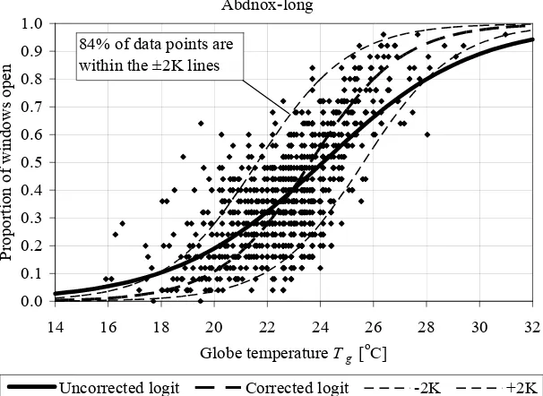
temperature. The proportion of windows open in the longitudinal survey is plotted as a scatter
diagram against the indoor temperature at the time of voting (Figure 7). Each point shows the
proportion of windows open at a particular room temperature. The logistic regression line,
predicting the probability of a window being open against the room temperature, although
giving an unbiased statistical prediction of the window opening, does not adequately
attributed to the binomial error in the probabilities. This inadequacy is attributable to the
dynamic of the window opening: a proportion of the windows are opened in response to a
rising room temperature. Only if the room cools enough to cause discomfort need more
windows again be closed. The proportion open will therefore remain much the same so long
as the room temperature remains within the deadband. The envelope of the points therefore
indicates the width of the temperature deadband.
This dynamic gives a horizontal structure to the data, so that the regression equation of the
room temperature on the logit of the window opening becomes the more appropriate
description of the data, rather than the logistic regression curve. This equation was calculated,
and the regression gradient adjusted to make allowance for the binomial error in the predictor
variable (the logits) arising from the sample size of only 25. (For a treatment of regression
with measurement errors see Cheng and Van Ness 1999). The symbols of the equations and
the values of the parameters are given in the Table 4, together with a note on the calculation
of the adjustment, since the method is not commonly used and may be unfamiliar.
In Figure 7, 84% of the data points are within ±2 K of the central line and so a 4 K zone was
adopted as the width of the deadband. (This is close to ±1.5 standard deviations of the
horizontal scatter of the points, a conventional estimate for the range.) The decision to include
some 80% of the points is a matter of judgment, and may need to be modified in the light of
further experience.
Near Here: Figure 7 and Table 4.
Implementation of window opening algorithm in ESP-r
A separate paper has described how the Humphreys algorithm (Appendix 1) for window
opening was derived from analysis of extensive survey data (Rijal et al. 2007) and its
implementation in the ESP-r dynamic simulation software. In this work a behavioural
algorithm for window opening, developed from field survey data has been implemented in
ESP-r. The algorithm is in alignment with the CEN standard for adaptive thermal comfort.
The comfort temperature was calculated from exponentially weighted running mean outdoor
temperature for a day (Trm) (CIBSE 2006).
For Trm>10oC: Tcomf = 0.33 Trm+ 18.8 (1)
For Trm≤10oC: Tcomf = 0.09 Trm+ 22.6 (2)
Multiple logistic regression analysis of windows open on both indoor globe temperature Tg
and outdoor air temperature Tao_igave rise to an equation for use to predicted window opening
(Rijal et al. 2007):
log(p/1−p)=0.171Tg+0.166Tao i−6.4 (3)
A comfort zone of ±2 K about the comfort temperature is used to represent the range of
internal conditions under which the occupant is likely to be comfortable (Nicol and
Humphreys 2007).
The office model
The chosen baseline cellular office faces south and is constructed to represent a typical 1990’s
office with a 22.5 m2 floor area within a thermally lightweight building (Figure 8). The
construction of the external wall, floor and ceiling is shown in Figure 9. The area of the
windows is 3.9 m2. The adaptive window opening algorithm is applied in the weekday office
and were closed all day at the weekend. Only trickle ventilation is allowed when the window
is closed.
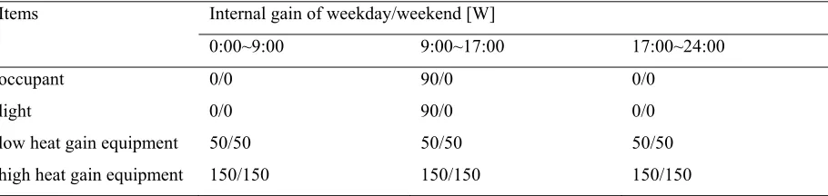
The heat gain from equipment is the same for weekdays and weekends. The heat gain from
occupants and lighting is applied only during weekdays (Table 5). The office has south facing
windows, occupant gains are set at 90 W during occupied hours, lighting gains at 90 W
during occupied hours and equipment gains at a constant 50 W. The combination of solar,
occupant and equipment gains gives a value of 36.6 W/m2 using the TM37 calculation
method (CIBSE TM37 2006). This is within the 30 to 40 W/m2 range where natural
ventilation is thought to be effective and just above the current UK building regulation
threshold of 35 W/m2 .
The cooling effects of window opening were simulated for four cases with different building
constructions: A) baseline, B) baseline + high thermal mass (plasterboard is replaced by 100
mm concrete ceiling), C) baseline + external shade (1.25 m projection from the wall) and D)
baseline + high thermal mass + external shade. They were simulated with low (50 W) and
high (150 W) heat gain equipment. (Most of the investigated buildings in the surveys were
similar to cases A and B.) Glazing is of a standard double glazing type as used in the 1990s.
The internal walls are plasterboard partitions.
For simulation, Gatwick climate data were used to evaluate the cooling effect of opening
windows while Dundee climate climate data were used for to evaluate summer overheating
because these data are located in a similar climate zone to Oxford and Aberdeen. The outdoor
temperatures and solar gains are similar over the four investigated days (Figure 10). Running
mean outdoor temperatures were calculated using 26 previous days of climate data, and the
full simulations were run over a start-up period of 6 days prior to the weekend period of
Near Here: Figures 8, 9 and Table 5.
Cooling effect of opening windows
To investigate the cooling effect of window opening, the thermal environment on weekdays
and weekends is predicted using ESP-r. For the unshaded office, the indoor temperatures are
high, triggering window opening early and delivering up to 500 W of cooling power (Figure
10 and Table 6). For the unshaded office, the indoor temperatures are higher during weekends
because the loss of cooling power is larger than the reduction in occupant and lighting gains.
For the shaded office, the indoor temperature is generally cooler (Figure 11 and Table 6).
When windows are opened there is less cooling energy because of the smaller indoor-outdoor
temperature difference. The window opening also occurs much later and, overall, delivers less
cooling. For the shaded office the effect at the weekend is that the reduction in heat gain from
occupants and lighting is similar in magnitude to the loss of cooling because windows are
closed. Thus, the temperature during weekdays is similar to the weekend in the shaded office.
The difference between weekday and weekend operative temperatures can be explained partly
by looking at a simple energy balance (Table 7). In general when there are higher average
total gains (losses) then indoor temperatures will tend to be higher.
The cooling effect of the open windows is higher in the lightweight building (case A)
compared with the heavyweight building (case B). Having windows open is also effective in
decreasing the indoor temperature when the internal gain is high. As mentioned above, there
may also be an air movement or fresh air advantage. For cases A, A’, B and B’, the minimum,
maximum, mean and SD of operative temperature of the weekday is lower than at the
weekend (Figure 10 and Table 6). The results show that having the windows open is not only
useful for reducing the mean indoor temperature but also useful for reduce the minimum and
the field investigation. It can be said from the simulation that the window opening behaviour
is highly important for the cooling of NV buildings.
Near Here: Figures 10, 11 and Table 6 & 7.
Summer overheating
The model was run through annual simulations with the Humphreys adaptive algorithm
controlling the window opening. Detailed results of time, temperature and energy flows for a
summer’s day are shown in Figure 12. In this case the window is opened at noon when the
operative temperature is close to 26oC. The outdoor temperature peaks at 23oC at 14:00 while
the indoor operative temperature peaks at 27oC around 16:00.
It is common in the study of the summer performance of naturally ventilated buildings to
assume that windows will begin to be opened in the summer when the indoor operative
temperature reaches some threshold and then opened proportionally until fully open when
some higher threshold is reached. In this analysis, this approach is termed ‘proportional’ and
is contrasted with the ‘adaptive’ approach of the Humphreys algorithm. This proportional
opening behaviour is illustrated in Figure 13, which shows windows beginning to open at
20oC and becoming fully open at 21oC for the same baseline office. The windows are open
earlier for this assumption than for the Humphreys algorithm (Figure 12). The thresholds
chosen here are towards the low end but within the range commonly used to demonstrate the
capability of a building in the UK to achieve an overheating specification.
Comparing the proportional approach to the adaptive behavioural algorithm over the summer
period shows significant differences as illustrated in Figure 14 and Figure 15. The
proportional approach gives lower peak temperatures and much lower temperature
For this example, the proportional approach gives a more optimistic prediction than the
Humphreys algorithm. The difference appears to be that in the proportional case the window
opening occurs before a discomfort triggered window opening event occurs. The Humphreys
algorithm, which is survey based and building and climate specific, is more likely to represent
actual behaviour than an arbitrary threshold that, in the absence of established criteria, would
be likely to be set at the most advantageous value.
Using the proportional approach in this way could lead to the assumption that the lightweight
unshaded office performance would prove acceptable. However, the Humphreys algorithm
identifies that the risk of overheating in the no shade or shaded office would be significant.
Moving ahead with a design based on the proportional approach would result in a significant
risk that occupants would experience discomfort leading to the need for remedial measures
such as fans, air conditioning or glazing replacement.
The integration of the algorithm and the adaptive comfort criteria within the dynamic
simulation tool allows comfort and behaviour in a given situation to be modelled as well as
the effect of behaviour for any given situation. In this case the window opening behaviour is
implemented within a dynamic thermal model. This means that occupant behaviour will
influence ventilation in a dynamic manner allowing design modifications to be made in
response to issues found.
Near Here: Figures 12, 13, 14 & 15
Further application of the algorithm
The algorithm was shown previously by the authors to give window opening results across all
4 seasons similar to those extracted from survey data (Rijal et al. 2007). The impact of the
also shown to be more sensitive to changes in building parameters than a standard non
adaptive approach. The building design and operational drivers of commonly observed
behaviours (such as having windows open while the heating is on in winter season) can begin
to be comprehended at an early stage in the design process . The algorithm generally suggests
that more comfortable buildings tend to be more energy efficient (less heating energy waste in
winter, lower risk of AC in summer).
It is suggested that an adaptive algorithm will better represent human control of windows and
allow a more accurate assessment of human thermal comfort conditions and building
performance, including summer overheating and annual energy use. The algorithm embedded
in simulation software will assist in the design of more comfortable and energy efficient
buildings. In order to illustrate the operation of the algorithm the data presented in this paper
has been taken from the application of the algorithm in a single throw deterministic-like
mode. In future applications to real building design, the algorithm should be deployed within
a structured multiple simulation methodology that accounts for the stochastic nature of the
algorithm and variations/uncertainties in input parameters (e.g. gains, climate) in order to
produce outputs representing realistic distributions of energy use and occupant comfort. The
approach is intended to be extended and integrated with adaptive behaviours such as lighting
and shading use, heating and cooling controls adjustment, use of fans and doors etc.
CONCLUSIONS
The window opening data from the field surveys showed the following principal features.
1) The mean Tg and Tao_i when the window is open are higher than when the window is
closed. This suggests that people are opening the window in response to increases in the
indoor and outdoor temperature, and that this effect conceals the cooling effect of window
2) The lower (≤10%) and upper (≥90%) limit of the cumulative Tg and Tao_i when windows
are open is higher than for when they are closed. The temperature range over which
windows are opened is wide.
3) The measured Tg of the weekdays (windows open) is lower than for the weekends
(windows closed). The results show that window opening had a significant cooling effect.
The method of calculating the ‘deadband’ for window opening is explained. A similar method
can be used in other data analysis situations, such as the use of fans (Rijal et al. 2007b, Nicol
et al. 2007).
The cooling effect of the window opening was verified by thermal simulation, using an
adaptive algorithm for window opening behaviour derived from field investigations. The
simulation results are compatible with field observations and show that window opening is
effective for cooling by controlling the internal and external heat gains in summer and by
increasing indoor air movement. Thus, window opening is useful to mitigate summer
overheating. An adaptive algorithm for window opening behaviour can be used in building
simulation to help design buildings that achieve thermal comfort and energy saving.
ACKNOWLEDGMENT
The research described was funded by the Engineering and Physical Sciences Research
Council (EPSRC). We are grateful to our former colleagues Kate McCartney and Professor
Iftikhar Raja, who collected and uploaded the data, and to the 890 people who took part in the
field study.
REFERENCES
Bourgeois D, Reinhart C, Macdonald I. 2006. Adding advanced behavioural models in whole
building energy simulation: a study on the total energy impact of manual and automated
lighting control, Energy and Buildings 38, 814-823.
Brager GS, Paliaga G and de Dear R. 2004. Openable windows, personal control and
occupant comfort, ASHRAE Transactions 110 (2), 17-35.
BRE. 2005. The UK Governments Standard Assessment Procedure SAP2005.
CEN 15251. 2007. Indoor environmental criteria for design and calculation of energy
performance of buildings. Comite Europeen de Normalisation, Brussels.
Cheng C-L and Van Ness JW. 1999. Statistical regression with measurement error, Library of
Statistics 6, Arnold, London.
CIBSE. 2006. Guide A, Environmental design, 7th Edition London, Chartered Institution of
Building Services Engineers.
CIBSE TM37. 2006. Design for improved shading control, London, Chartered Institution of
Building Services Engineers.
Fritsch R, Kohler A, Nygard-Ferguson M and Scartezzini JL. 1990. A stochastic model of
user behaviour regarding ventilation, Building and Environment 25 (2), 173-181.
Herkel S, Knapp U and Pfafferott J. 2007. Towards a model of users behaviour regarding the
manual control of windows in office buildings, Building and Environment, (in press)
doi:10.1016/j.buildenv.2006.06.031.
Humphreys MA. 1973. Classroom temperature, clothing and thermal comfort - a study of
Humphreys MA and Nicol JF. 1995. An adaptive guideline for UK office temperatures, in:
Standards for thermal comfort: Indoor air temperature standards for the 21st century, pp.
190-195, E & FN Spon.
Hunt DRG. 1979. The use of artificial lighting in relation to daylight levels and occupancy,
Building and Environment 14, 21-33.
Inkarojrit V and Paliaga G. 2004. Indoor climatic influences on the operation of windows in a
naturally ventilated buildings, Proceedings of the 21th International Conference on Passive
and Low Energy Architecture, Netherlands, September 19-22.
McCartney KJ and Nicol JF. 2002. Developing an adaptive control algorithm for Europe,
Energy and Buildings (34), 623-635.
Newsham GR, Mahdavi A, Beausoleil-Morrison I. 1995. Lightswitch: a stochastic model for
predicting office lighting energy consumption, Proceedings of Right Light Three, the
Third European Conference on Energy Efficient Lighting, Newcastle-upon-Tyne, 60-66.
Nicol JF, Raja IA, Allaudin A and Jamy GN. 1999. Climatic variations in comfortable
temperatures: the Pakistan projects, Energy and Buildings 30 (3), 261-279.
Nicol JF. 2001. Characterising occupant behaviour in buildings: towards a stochastic model
of occupant use of windows, lights, blinds, heaters and fans, Proceedings of the seventh
international IBPSA conference (Brazil), pp 1073-1078.
Nicol JF and Humphreys MA. 2004. A stochastic approach to thermal comfort, occupant
behaviour and energy use in buildings, ASHRAE Transactions 110(2), 554-568.
Nicol F and Humphreys M. 2007. Maximum temperatures in European office buildings to
Nicol JF, Rijal HB, Humphreys MA and Tuohy P. 2007. Characterising the use of windows in
thermal simulation, 2nd PALENC Conference and 28th AIVC Conference on Building Low
Energy Cooling and Advance Ventilation Technologies in the 21st century, Greece,
September 27-29, pp. 712-717.
Olesen B. 2007. The philosophy behind EN15251: Indoor environmental criteria for design
and calculation of energy performance of buildings, Energy and Buildings 39 (7),
740-749.
Pfafferott J and Herkel S. 2007. Statistical simulation of user behaviour in low-energy offices
buildings, Solar Energy 81 (5), 676-682.
Raja IA, Nicol JF, McCartney KJ and Humphreys MA. 2001. Thermal comfort: use of
controls in naturally ventilated buildings, Energy and Buildings 33 (3), 235-244.
Reinhart CF. 2004. Lightswitch-2002: a model for manual and automated control of electric
lighting and blinds, Solar Energy 77, 15-28.
Rijal HB, Tuohy P, Humphreys MA, Nicol JF, Samuel A and Clarke J. 2007. Using results
from field surveys to predict the effect of open windows on thermal comfort and energy
use in buildings, Energy & Buildings, 39 (7), 823-836.
Rijal HB, Tuohy P, Nicol F, Humphreys MA and Clarke J. 2007a. A window opening
algorithm and UK office temperature: Field results and thermal simulation, Proceedings of
the 10th International IBPSA Conference, Beijing, September 3-6, pp. 709-716.
Rijal HB, Nicol F, Humphreys M and Raja IA. 2007b, Use of windows, fans and doors to
control the indoor environment in Pakistan: Developing a behavioural model for use in
thermal simulations, the 2nd International Conference of Environmentally Sustainable
Robinson D and Haldi F. 2007. An integrated adaptive model for overheating risk prediction,
Proceedings of the 10th International IBPSA Conference, Beijing, September 3-6, pp.
745-750.
Tuohy P, Rijal HB, Humphreys MA, Nicol JF, Samuel A and Clarke J. 2007. Comfort driven
adaptive window opening behaviour and the influence of building design, Proceedings of
the 10th International IBPSA Conference, Beijing, September 3-6, pp. 717-724.
Yun GY and Steemers K. 2007. Time-dependent occupant behaviour models of window
control in summer, Building and Environment, (in press)
doi:10.1016/j.buildenv.2007.08.001.
Warren PR and Parkins LM. 1984. Window-opening behaviour in office buildings, ASHRAE
[image:22.595.64.532.453.553.2]Transactions 90(1B), 1056-1076.
Table 1 Values of globe temperature and outdoor air temperature for windows open and
closed in the longitudinal and transverse surveys.
Temp. [oC] Window Abdnox-long Abdnox-trans
N [-] Min Max Mean SD N [-] Min Max Mean SD
Tg closed (0) 13,702 8.8 30.6 22.2 1.8 2,296 18.1 28.6 23.1 1.4
open (1) 8,784 15.6 33.5 23.4 2.0 1,156 16.7 29.5 24.0 1.6
Tao_i closed (0) 15,610 -6.4 30.8 9.7 5.5 2,308 -2.0 26.6 11.5 5.6
open (1) 9,706 -2.4 30.7 15.6 5.9 1,122 -1.9 26.6 16.4 5.5
Table 2 Globe temperatures and outdoor air temperatures for percentile points when
windows are open and closed.
Temp. [oC] Window Abdnox-long Abdnox-trans
N [-] Cumulative value N [-] Cumulative value
10% 50% 90% 10% 50% 90%
Tg closed (0) 13,702 19.8 22.4 24.3 2,296 21.4 22.9 24.8
open (1) 8,784 20.9 23.3 26.0 1,156 21.9 23.8 26.1
Tao_i closed (0) 15,610 2.7 9.8 16.6 2,308 4.1 12.0 18.7
[image:22.595.64.533.626.740.2]Table 3 Values of globe temperature and outdoor air temperature for windows open and
closed (01-pair and 10-pair) in longitudinal surveys.
Temp. [oC] Window 01-pairs 10-pairs
N [-] Min Max Mean SD N [-] Min Max Mean SD
Tg closed (0) 1,316 12.6 28.6 22.5 1.6 487 17.7 28.4 23.0 1.6
open (1) 1,316 17.8 31.4 23.1 1.6 487 15.6 27.8 22.7 1.8
Tao_i closed (0) 1,469 -2.4 25.9 11.6 5.2 580 0.1 30.5 11.5 5.5
open (1) 1,469 -0.8 28.4 12.8 5.4 580 -1.1 30.7 11.6 5.3
Table 4 Symbols and values of parameters used to calculate the adjusted regression equation,
based on the records grouped in 25s.
Parameter Symbol Value
Globe temperature Tg -
Logit of the windows open logit -
Regression coefficient of Tg on logit b 1.33
Variance of logit var(logit) 1.062
Covariance of Tg and logit cov(Tg, logit) 1.412
Number of sample size n 25
Proportion of windows open p 0~1
Mean variance of logit error var(logit error) 0.2378
Mean logit logitm -0.5303
Mean globe temperature Tgm 22.7
Residual of Tg - 1.36836
Notes: Steps in obtaining the adjusted equation:
b=cov(Tg, logit)/var(logit) (1)
hence cov (Tg, logit)=b×var(logit) (2)
and var(logit error)= 1/{np(1−p)} (3)
[image:23.595.70.529.457.668.2]hence Tg=1.713logit+c (5)
so logit=0.584Tg+c (6)
The equation must pass through the group means of Tg and the logit, thus c=logitm−0.584Tgm (7)
The centre line of the deadband:
logit=0.584Tg−13.8 (8)
the width of deadband is taken as ±1.5SD×Residual of Tg (9)
So the equations for deadband margins are:
logit=0.584(Tg±2.1) −13.8 (10)
[image:24.595.72.527.261.369.2]but p=e(logit)/{1+e(logit)} so the curves may now be drawn (11)
Table 5 Schedule of the internal gains.
Items Internal gain of weekday/weekend [W]
0:00~9:00 9:00~17:00 17:00~24:00
occupant 0/0 90/0 0/0
light 0/0 90/0 0/0
low heat gain equipment 50/50 50/50 50/50
high heat gain equipment 150/150 150/150 150/150
Table 6 Operative temperature in the office hour (9:30 ~ 17:30) of weekday and weekend.
Case Operative temperature [oC] Weekday−Weekend [K]
Weekday Weekend
Min Max Mean S
D
Min Max Mean SD Min Max Mean SD
A 21.2 31.2 28.1 2.7 23.3 33.3 29.7 3.4 -2.1 -2.1 -1.7 -0.7
A’ 22.7 31.8 29.0 2.4 24.9 34.9 31.3 3.5 -2.2 -3.1 -2.3 -1.1
B 22.3 30.4 27.9 2.1 24.5 31.6 29.0 2.3 -2.2 -1.2 -1.2 -0.2
B’ 23.7 31.2 28.7 1.9 25.9 33.1 30.5 2.3 -2.2 -1.9 -1.8 -0.4
C 20.0 28.1 25.3 2.5 21.7 27.7 25.1 2.0 -1.7 0.4 0.2 0.5
C’ 21.5 28.8 26.3 2.2 23.3 29.3 26.6 2.0 -1.8 -0.5 -0.3 0.1
D 21.2 27.4 25.2 1.8 22.8 26.5 25.0 1.3 -1.6 0.9 0.2 0.5
D’ 22.6 28.3 26.4 1.6 24.3 28.1 26.5 1.3 -1.6 0.1 -0.2 0.2
[image:24.595.67.530.423.639.2]Table 7 24hr average heat flows due to solar / casual gains and infiltration losses for the
same cases as in Table 6.
Case Average gains / losses of 24 hour [W] Weekday−Weekend [W]
Weekday Weekend
Sol Inf Cas Total Sol Inf Cas Total Sol Inf Cas Total
A 174 -117 110 167 174 -2 50 222 0 -115 60 -55
A’ 174 -145 210 240 174 -3 150 321 0 -142 60 -82
B 174 -92 110 193 174 -2 50 222 0 -90 60 -29
B’ 174 -125 209 258 174 -2 150 321 0 -123 59 -62
C 91 -45 110 156 88 -2 50 136 4 -43 60 20
C’ 91 -70 210 232 88 -2 150 236 4 -67 60 -4
D 91 -32 110 169 88 -1 50 136 4 -31 60 33
D, 91 -54 210 247 88 -2 150 236 4 -52 60 11
Sol: Solar gain, Inf: Infiltration losses, Cas: Occupant, lighting and equipment gain
14 -S H 13 -S N 11-GH 9-V W 8-R P 7-G T 6-CL 4-B H 2-A L 1-M F Buildings 26 25 24 23 22 21 20 19 Gl obe temp. [C]
○: windows open ●: windows closed
○: windows open ●: windows closed
(a) Abdnox-long 14 -S H 13 -S N 11 -G H 9-VW 8-R P 7-GT 6-C L 4-BH 2-AL 1-MF Buildings 26 25 24 23 22 21 20 19 Gl ob e te m p. [ C ]
○: windows open ●: windows closed
○: windows open ●: windows closed
14 -S H 13 -S N 11 -G H 9-VW 8-R P 7-GT 6-C L 4-BH 2-AL 1-M F Buildings 24 21 18 15 12 9 6 Ou tdo or temp . [ C
] ○○: windows open : windows open ●●: windows closed: windows closed
(c) Abdnox-long 14 -S H 13 -S N 11 -G H 9-V W 8-R P 7-G T 6-C L 4-B H 2-A L 1-M F Buildings
○: windows open ●: windows closed
○: windows open ●: windows closed
24 21 18 15 12 9 6
Outdoor temp. [C
]
[image:26.595.77.280.77.326.2](d) Abdnox-trans
Figure 1 Comparison of mean globe temperature and outdoor air temperature with 95%
confidence intervals for windows open (open symbols) and closed in longitudinal and
(c) Abdnox-long: Tao_i 0 20 40 60 80 100
-5 0 5 10 15 20 25 30
Tao_i [oC]
Pr opor tion [ % ] windows closed n=15,610 windows open n=9,706 (a) Abdnox-long: Tg
0 20 40 60 80 100
16 18 20 22 24 26 28 30
Tg [oC]
Pr opor tion [ % ] windows open n=8,784 windows closed n=13,702
(b) Abdnox-trans: Tg
0 20 40 60 80 100
16 18 20 22 24 26 28 30
Tg [oC]
Pr
opor
tion
[
%
] windows closed
n=2,296
windows open n=1,156
(d) Abdnox-trans: Tao_i
0 20 40 60 80 100
-5 0 5 10 15 20 25 30
Tao_i[oC]
[image:27.595.78.298.76.657.2]Pr opor tion [ % ] windows open n=1,122 windows closed n=2,308
Figure 2 Cumulative distributions of globe temperature and outdoor air temperature for NV
14-S H 13-S N 11-G H 9-V W 8-R P 7-GT 6-C L 4-B H 2-AL 1-MF Buildings 26 25 24 23 22 21 20 19 Globe te mp. [C]
○: windows open ●: windows closed
○: windows open ●: windows closed
(a) 01-pair 14-S H 13-S N 11-GH 9-VW 8-RP 7-GT 6-C L 4-BH 2-AL 1-MF Buildings 24 21 18 15 12 9 6 Outdoor t emp. [C ]
○: windows open ●: windows closed
○: windows open ●: windows closed
(b) 01-pair 14 -S H 13 -S N 11-G H 9-V W 8-R P 7-G T 6-CL 4-B H 2-A L 1-M F Buildings 26 25 24 23 22 21 20 19 Globe tem p. [C ]
○: windows open ●: windows closed
○: windows open ●: windows closed (c) 10-pair 14 -S H 13 -S N 11 -GH 9-V W 8-R P 7-G T 6-C L 4-B H 2-A L 1-M F Buildings 24 21 18 15 12 9 6 Outdoor temp. [ C ]
○: windows open ●: windows closed
○: windows open ●: windows closed
[image:28.595.77.281.70.619.2](d) 10-pair
Figure 3 Comparison of mean globe temperature and outdoor air temperature with 95%
confidence intervals for windows open (open symbols) and closed at adjacent times in the
9-V W /9 .550/M 8-RP /8.110/ M 4-BH/4.22 0/M 9-V W /9.480/ S 9-V W /9.450/ S 9-V W /9.120/ S 7-GT /7 .090/S 6-CL/6.160/S 4-BH /4.4 60/S 4-BH /4.3 10/S 9-V W /9.210/A 9-V W /9.070/A 8-RP /8.100/ A 7-GT /7 .190/A 4-BH /4.3 10/A 4-BH /4.1 30/A Building/Subject/Month 30 28 26 24 22 20 Glo be te mp. [C]
○: windows open ●: windows closed
○: windows open ●: windows closed
[image:29.595.81.320.78.297.2]Abdnox-long
Figure 4 Comparison of mean globe temperatures with 95% confidence intervals in the
buildings when windows are open (weekdays: open symbols) and closed (weekends) in
longitudinal survey, after adjustment for air movement and heat gains. A: Aug. (16th to 19th,
1996), S: Sept. (13th to 16th, 1996) M: May-Jun (30th to 2nd, 1997).
Abdnox-long 0 20 40 60 80 100
16 18 20 22 24 26 28 30
Tg [oC]
Pr op or tio n [ % ] windows closed (weekend) windows open (weekday)
Figure 5 Cumulative distribution of the globe temperature during weekdays (windows open)
and weekends (windows closed) in longitudinal survey, after adjustment for air movement and
y = 0.7598x + 3.9018 R2 = 0.7465
20 22 24 26 28 30
20 22 24 26 28 30
Tg of windows closed [oC] Tg
of w
in
dow
s open [
[image:30.595.81.316.76.311.2]o C]
Figure 6 Comparison of Tg for the windows open and closed for each person in weekday and
weekend.
Abdnox-long
0.0 0.1 0.2 0.3 0.4 0.5 0.6 0.7 0.8 0.9 1.0
14 16 18 20 22 24 26 28 30 32
Globe temperature Tg [oC]
P
roportion o
f
windows op
en
Uncorrected logit Corrected logit -2K +2K 84% of data points are
within the ±2K lines
Figure 7 Logistic regression curve for windows open as a function of globe temperature in all
NV buildings in longitudinal surveys, and the adjusted lines showing the margins of the
[image:30.595.79.382.382.603.2]N
N
Figure 8 Representation of the cellular office (labelled ‘office’) located within the larger
open plan office area (labelled ‘corridor’). The office window faces south(Note that the
cellular office showing the external shade above the office window for case C).
211
(a) wall (c) ceiling
carpet (5)
(b) floor Indoor
insulation (105)
O
utdoo
r
Indoor
br
ick
(
100
)
ai
r g
ap
(50
)
pl
as
te
rbo
ard
(13)
pl
as
te
r
(3)
in
su
latio
n
(45)
plaster (3) timber (7.5) insulation (74)
plasterboard(13)
Figure 9 Construction of the wall, floor and ceiling for baseline case (A). The thickness of the
Case A: Baseline (low heat gain equipment) 0 5 10 15 20 25 30 35
00:30 00:30 00:30 00:30 Time [h]
T em pe ra tu re [ o C] -500 0 500 1000 1500 2000 2500 3000 In filtr at
ion and gain [W]
Operative temp. Outdoor temp.
Infiltration Internal gain
[image:32.595.81.362.81.325.2]Solar gain
Figure 10 Temperatures and energy flows for weekday and weekend (July 19 Friday ~ July 22 Monday, 1991, Gatwick, UK). The lines represent the outdoor air temperature, the indoor operative temperature (with symbols) and the energy flows from the convective cooling by the incoming air, the heat gains from occupants, lights and equipment and the incoming direct solar heating absorbed in the indoor surfaces of the office.
Case C: Baseline + shade (low heat gain equipment)
0 5 10 15 20 25 30 35
00:30 00:30 00:30 00:30 Time [h]
Temper atur e [ o C] -500 0 500 1000 1500 2000 2500 3000 In filtratio
n and g
ain [W]
Operative temp. Outdoor temp. Infiltration Internal gain Solar gain
[image:32.595.82.371.462.704.2]0 5 10 15 20 25 30
00:30 04:30 08:30 12:30 16:30 20:30
Time [h] Temperature [ o C] -300 -100 100 300 500 700 900 Infi lt rat io
n and gai
n
[W]
Outdoor temp. Operative temp. Infiltration Internal gains Solar gain
Figure 12 Temperature, heat gains and ventilation losses for a summer day modeled using the
Humphreys algorithm (Case A).
0 5 10 15 20 25 30
00:30 04:30 08:30 12:30 16:30 20:30 Time [h] Tem perat ur e [ o C] -300 -100 100 300 500 700 900 In filtra tion a nd ga in [W]
Outdoor temp. Operative temp. Infiltration Internal gains Solar gain
Figure 13 Temperatures, gains and losses for a summer day with window opening behavior
20 22 24 26 28 30
no shade shaded shade + mass
Model
Peak
te
m
perat
ur
e [
o C]
adaptive proportional
Figure 14 Peak operative temperatures for the summer season modeled using the Humphreys
algorithm (adaptive) and the threshold method (proportional) (no shade=baseline (Case A)).
0 4 8 12 16 20
no shade shaded shade + mass Model
Percentage of occupied hours [%]
[image:34.595.91.473.108.342.2]adaptive proportional
Figure 15 Percentage of occupied hours with operative temperatures over 26oC for adaptive
Appendix 1 Steps in the implementation of the ‘Humphreys’ adaptive window open algorithm
in ESP-r (Rijal et al. 2007).
No. Window algorithm parameter Symbol Sample Derivation or source
1 Outdoor air temp. Tout 1/h Interpolated from climate file (hourly data in file)
2 Daily mean outdoor air temp. Todm 1/day Calculated from 24 hourly data points per day
3 Running mean outdoor air temp. (CEN) Trm 1/day Trm(init) = (1−α){Todm−1+ αTodm−2 + α2Todm−3…}
Initial value calculated from previous 20 days daily mean then Trm = (1−α)Todm−1+ αTrm−1
4 Running mean response to Tout α Const Default α = 0.8 (0.01 to 0.99 allowed range)
5 Comfort temp. Tcomf 1/day If Trm>10, Tcomf = 0.33Trm + 18.8 (CEN standard)
If Trm≤10, Tcomf = 0.09Trm + 22.6
6 Indoor air temp. Tai 1/h Available at each timestep (variable)
7 Indoor operative temp. Top 1/h Available at each timestep (50% mrt, 50% Tai)
8 Comfort Comf 1/h Comf = ‘yes’ if abs (Top−Tcomf)≤2K
Comf = ‘hot’ if (Top−Tcomf)>2K
Comf = ‘cold’ if (Top-Tcomf)<−2K
9 Logit function Func 1/h Func = Logit(Pw) = 0.171Top + 0.166Tout− 6.43
10 Probability function for window open Pw 1/h Pw = exp(Func)/{1+exp(Func)}
11 Random number between 0 and 1 Rn 1/h Generated from fortran RNG