On Testing Global Optimization Algorithms for Space
Trajectory Design
M. Vasile
∗and E. Minisci
†University of Glasgow, Glasgow, G12 8QQ, United Kingdom
M. Locatelli
‡Universit`a degli Studi di Torino, Turin, 10149, Italy
In this paper we discuss the procedures to test a global search algorithm applied to a space trajectory design problem. Then, we present some performance indexes that can be used to evaluate the effectiveness of global optimization algorithms. The performance indexes are then compared highlighting the actual significance of each one of them. A number of global optimization algorithms are tested on four typical space trajectory de-sign problems. From the results of the proposed testing procedure we infer for each pair algorithm-problem the relation between the heuristics implemented in the solution algo-rithm and the main characteristics of the problem under investigation. From this analysis we derive a novel interpretation of some evolutionary heuristics, based on dynamical system theory and we significantly improve the performance of one of the tested algorithms.
I.
Introduction
In the last decade many authors have used global optimization techniques to find optimal solutions to space trajectory design problems. Many different methods have been proposed and tested on a variety of cases. From pure Genetic Algorithms1–4 to Evolutionary Strategies (such as Differential Evolution)5 to hybrid
methods,8 the general intent is to improve over the pure grid or enumerative search. Sometimes, the actual
advantage of using a global method is difficult to appreciate, in particular when stochastic based techniques are used. In fact, if, on one hand, a stochastic search provides a non-zero probability to find an optimal solution even with a small number of function evaluations, on the other hand, the repeatability of the result and therefore the reliability of the method can be questionable. The first actual assessment of the suitability of global optimization methods to the solution of space trajectory design problems can be found in two studies by the University of Reading7and by the University of Glasgow.6 The former presented a small set
of test problems mainly focusing on multiple gravity assist trajectories, while the latter included results for low-thrust transfers using a wide range of global optimizers. One of the interesting outcomes of both studies was that Differential Evolution, belonging to a subclass of Evolutionary Algorithms, performed particularly well on most of the problems, compared to other methods. In both studies, the indexes of performance for stochastic methods were: the average value of the best solution found for each run over a number of independent runs, the corresponding variance and the best value from all the runs. For deterministic methods, the index of performance was the best value for a given number of function evaluations. It should be noted that the application of global methods to space trajectory problems has often considered the problem as a black-box with limited exploitation of problem characteristics. On the other hand, ad hoc techniques exploiting problem characteristics7 provide a sensible improvement over the simple enumerative search.
In this paper, we propose a testing methodology for global optimization methods addressing specifically black-box problems in space trajectory design. In particular, we focus our attention on stochastic based approaches. The paper discusses the actual significance of some performance indexes and proposes some criteria to evaluate the actual usefulness of an algorithm. Furthermore, the paper presents a benchmark of
∗Senior Lecturer, Aerospace Engineering, James Watt South Building, AIAA Member.
†Research Fellow, Aerospace Engineering, James Watt South Building.
test cases, and an analysis of the relationship between the heuristics implemented in some global optimization algorithms and the main characteristics of the test cases under investigation. The identification of common patterns in the relation between solution method and problem features represents a useful guideline for the selection of the most appropriate approach to a problem. From this analysis we derive a novel formulation of some evolutionary heuristics, based on dynamical system theory and we propose a modified version of Differential Evolution that improves significantly over the standard DE. It is worth to underline that this paper does not intend to propose any particular benchmark for testing global optimization algorithms, nor it wants to prove that one approach is better than the others. The goal of this paper is instead to propose a method of assessment and analysis of stochastic methods for global optimization applied to space trajectory design problems. A correct analysis of the performance of a particular method applied to a specific class of problem can be useful to identify which heuristic is most effective.
II.
Problem Description
We consider a benchmark made of four different test-cases, with increasing complexity: a direct bi-impulsive transfer from the Earth to an asteroid, a transfer to Mars via a gravity assist of Venus, a multi-gravity assist transfer to Saturn with no mid-course manoeuvres and the same transfer but with mid-course manoeuvres. In all of these cases the objective will be to minimize the total variation of the velocity of the spacecraft due to all propelled maneuvers, or total ∆v.
II.A. Bi-impulsive Earth-Apophis Transfer
A simple, but already significant, application is to find the best launch datet0and time of flightTto transfer
a spacecraft from the Earth to the asteroid Apophis. The transfer is computed as the solution of a Lambert’s problem.11 The objective function for this problem is the sum of the departure velocity change ∆v
iand the
arrival velocity change ∆vf:
f(x) = ∆vi+ ∆vf (1)
with the solution vector:
x= [t0, T]T (2)
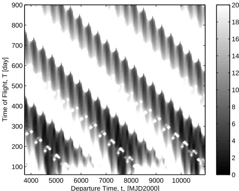
The search spaceDis a box defining the limits of the two components of the solution vector. In particular, the launch date from the Earth was taken in the interval [3653, 10958]MJD2000 (i.e. number of elapsed days since January 1st 2000), while the time of flight was taken in the interval [50, 900] days. A representation of the search space can be seen in Fig.1 where the value of the objective function was plotted with level curves againstt0 andT: dark regions represent local minima.
The known best solution inD isfbest=4.3745658 km/s,xbest=[10027.6215924826, 305.12163547522].
II.B. Earth-Venus-Mars Transfer with DSM
The second test-case consists of a transfer from Earth to Mars with the use of a gravity assist manoeuvre at Venus and a deep-space manoeuvre (DSM) after Venus. This is the simplest instance of a multi-gravity assist trajectory with deep-space manoeuvres (MGA-DSM).
II.B.1. Trajectory Model
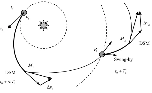
A general MGA-DSM trajectory can be modeled through a sequence ofNP−1 legs connectingNP celestial
bodies (Fig. 2).9 In particular if all celestial bodies are planets, each leg begins and ends with an encounter
with a planet. Each legiis made of two conic arcs: the first, propagated analytically forward in time, ends where the second, solution of a Lambert’s problem, begins. The two arcs have a discontinuity in the absolute heliocentric velocity at their matching point M. Each DSM is computed as the vector difference between the velocities along the two conic arcs at the matching point. Given the transfer time Ti and the variable
αi ∈ [0,1] relative to each leg i, the matching point is at timetDSM,i =tf,i−1+αiTi, where tf,i−1 is the
final time of the legi−1. The relative velocity vectorv0 at the departure planet can be a design parameter
and is expressed as:
Departure Time, t
0 [MJD2000]
Time of Flight, T [day]
4000 5000 6000 7000 8000 9000 10000 100
200 300 400 500 600 700 800 900
0 2 4 6 8 10 12 14 16 18 20
Figure 1. Earth-Apophis search space.
with the angles δ and θ respectively representing the declination and the right ascension with respect to a local reference frame with the x axis aligned with the velocity vector of the planet, the z axis normal to orbital plane of the planet and the y axis completing the coordinate frame. This choice allows easily constraining the escape velocity and asymptote direction while adding the possibility of having a deep space maneuver in the first arc after the launch. This is often the case when escape velocity must be fixed due to the launcher capability or to the requirement of a resonant swing-by of the Earth (Earth-Earth transfers). In order to have a uniform distribution of random points on the surface of the sphere defining all the possible launch directions, the following transformation has been applied:
¯ θ= θ
2π; ¯δ=
cos(δ+π/2) + 1
2 (4)
It results that the sphere surface is uniformly sampled when a uniform distribution of points for ¯θ,¯δ∈[0,1] is chosen. Once the heliocentric velocity at the beginning of leg i, which can be the result of a swing-by maneuver or the asymptotic velocity after launch, is computed, the trajectory is analytically propagated until
timetDSM,i. The second arc of legiis then solved through a Lambert’s algorithm, fromMi, the Cartesian
position of the deep space maneuver, toPi, the position of the target planet of phasei, for a time of flight
(1−αi)Ti. Two subsequent legs are then joined together with a gravity assist manoeuvre. The effect of the
gravity of a planet is to instantaneously change the velocity vector of the spacecraft. The relative incoming velocity vector and the outgoing velocity vector, at the planet swing-by, have the same modulus but different directions; therefore the heliocentric outgoing velocity results to be different from the heliocentric incoming one. In the linked conic model the spacecraft is assumed to follow a hyperbolic trajectory with respect to the swing-by planet. The angular difference between the incoming relative velocity ˜vi and the outgoing one ˜vo
depends on the modulus of the incoming velocity and on the pericenter radiusri. Both the relative incoming
and outgoing velocities belong to the plane of the hyperbola. However, in the linked-conic approximation, the maneuver is assumed to occur at the planet, where the planet is a point mass coinciding with its center of mass. Therefore, given the incoming velocity vector, one angle is required to define the attitude of the plane of the hyperbola Π. There are different possible choices for the attitude angleγ; the one proposed in Ref. 7 has been adopted (Fig. 3): γ is the angle between the vector nΠ, normal to the hyperbola plane Π,
and the reference vectornr, that is normal to the plane containing the incoming relative velocity and the
velocity of the planetvP.
Given the number of legs of the trajectoryNL=NP−1, the complete solution vector for this model is:
[image:3.612.176.420.65.260.2]Figure 2. Schematic representation of a multiple gravity assist trajectory
Figure 3. Schematic representation of a multiple gravity assist trajectory
wheret0 is the departure date. Now, the design of a multi-gravity assist transfer can be transcribed into a
general nonlinear programming problem, with simple box constraints, of the form:
min
x∈Df(x) (6)
One of the appealing aspects of this formulation is its solvability through a general global search method for box constrained problems. Depending on the kind of problem under study, the objective function can be defined in different ways. Here we choose to focus on the problem of minimizing the total ∆vof the mission, therefore the objective functionf(x) is:
f(x) =v0+ Np
∑
i=1
∆vi+ ∆vf (7)
where ∆vi is the velocity change due to the DSM in thei−thleg, and ∆vf is the maneuver needed to inject
the spacecraft into the final orbit.
For a transfer to Mars via Venus, the solution vector in Eq. (5) has six dimensions. In particular the initial velocity with respect to the Earth is not a free parameter but is computed as the result of the Lambert’s problem for the Earth-Venus leg. Therefore we can define the following reduced solution vector:
x= [t0, T1, γ1, rp,1, α2, T2] (8)
Since the initial velocity is not a free parameter, v0 is the modulus of the vector difference between the
velocity of the Earth at timet0and the velocity of the spacecraft at the same time. Note that the final ∆vf
[image:4.612.188.445.61.219.2] [image:4.612.242.373.279.382.2]radius and 0.98 of eccentricity. This choice does not alter the nature of the problem but scales down the contribution of the last impulsive manoeuvre. The search spaceD is defined by the following intervals: t0∈
[3650,9129] MJD2000,T1∈[50,400] d,γ1∈[−π, π], rp,1∈[1,5],α2∈[0.01,0.9],T2∈[50,700] d. The best
known solution for this problem in the given search spaceDisfbest=2.9811 km/s,xbest=[4472.01334656364,
172.289324250300, 2.97843388136061, 1, 0.509432880679500, 697.610012389372].
II.C. Earth-Saturn Transfer
The third test is a multi gravity assist trajectory from the Earth to Saturn following the sequence Earth-Venus-Venus-Earth-Jupiter-Saturn (EVVEJS). Gravity assist maneuvers are modeled through a linked-conic approximation with powered maneuvers,7i.e., the mismatch in the outgoing velocity is compensated through a ∆vmaneuver at the pericenter of the gravity assist hyperbola for each planet. No deep-space maneuvers are possible and each planet-to-planet transfer is computed as the solution of a Lambert’s problem. Therefore, the whole trajectory is completely defined by the departure timet0and by the transfer time for each legTi,
with i= 1, ..., NP−1. The radius of the pericenter rp,i of each swing-by hyperbola is derived a posteriori
once each powered swing-by manoeuvre is computed. Thus, a constraint on each pericenter radius has to be introduced during the search for an optimal solution. The trajectory model for this problem can be downloaded from the ESA/ACT websitea. In order to take into account the constraints on the altitude of
the pericenters the objective function is augmented with the weighted violation of the constraints:
f(x) = ∆v0+ N∑p−2
i=1
∆vi+ ∆vf+ N∑p−2
i=1
wi(rp,i−rpmin,i)2 (9)
with the solution vector:
x= [t0, T1, T2, T3, T4, T5] (10)
The weighting functionswi are defined as follows:
wi= 0.005[1−sign(rp,i−rpmin,i)], i= 1, ...,3
w4= 0.0005[1−sign(rp,4−rpmin,4)]
(11)
with the minimum pericenter radii rpmin,1 = 6351.8, rpmin,2 = 6351.8, rpmin,3 = 6778.1 and rpmin,4 =
671492. For this case the dimensionality of the problem is six, and the search space D is defined by the following intervals: t0 ∈ [−1000,0]MJD2000, T1 ∈ [30,400]d, T2 ∈ [100,470]d, T3 ∈ [30,400]d, T4 ∈
[400,2000]d,T5∈[1000,6000]d. The best known solution isfbest=4.9307 km/s,xbest=[-789.8055, 158.33942,
449.38588, 54.720136, 1024.6563, 4552.7531].
II.D. Earth-Saturn Transfer with DSMs
The forth test case is again a multi gravity assist trajectory from the Earth to Saturn following the sequence Earth-Venus-Venus-Earth-Jupiter-Saturn (EVVEJS) but a deep space manoeuvre is allowed along the trans-fer arc from one planet to the other. Although from a trajectory design point of view this problem is similar to problem three, the model is substantially different and therefore it represents a different problem from a global optimization point of view. Since the transcription of the same problem into different mathematical models can affect the search for the global optimum, it is interesting to analyze the behavior of the same set of global optimization algorithms applied to two different transcriptions of the same trajectory design problem.
The trajectory model for this test case can be downloaded from the ESA/ACT web site b. This model is very similar to the one for problem two, the only differences are in the definition of the attitude angle γ of the plane of the hyperbola, which is at 90 degrees with respect to the one of problem two, and in the computation of ∆vf that is now the modulus of the vector difference between the velocity of Saturn at
arrival and the velocity of the spacecraft at the same time. Although the difference is minimal we preferred to use the ESA/ACT version since for this problem some reference solutions are already available and therefore a comparison is easier and not affected by any difference in the implementation of the trajectory
ahttp://www.esa.int/gsp/ACT/inf/op/globopt/evvejs.htm
model. The best known solution isfbest=8.4091810440 km/s,xbest=[-779.060197373242, 3.32046443745595,
0.531333503613675, 0.376218447342955, 168.685775870437, 422.672656805198, 53.3360098337041,
589.777827855018, 2200, 0.718720247401635, 0.532962541494841, 0.159170896444411, 0.470495109020601, 0.0986526263521857, 1.46946051297954, 1.05138706406598, 1.30594027188689, 69.8194077461197,
-1.60160853231321, -1.9600386515463, -1.55445003054861, -1.51343200828766].
Note that, prior to run each test we normalized the search space for each one of the trajectory models so thatD is a unit hypercube with each component of the solution vector belonging to the interval [0,1].
III.
Optimization Algorithm Description
We tested five stochastic global search algorithms: Differential Evolution (DE) and Genetic Algorithms (GA) that belong to the generic class of Evolutionary Algorithms (EA), Particle Swarm Optimization (PSO) that belongs to the class of agent-based algorithms, and Multistart (MS) and Monotonic Basin Hopping (MBH) that are based on multiple local searches with a gradient method. In a previous paper by the authors27
we showed how deterministic algorithms, such as DIRECT,18 might work better then stochastic ones on
simple problems, such as the bi-impulsive case. On the other hand, for more complex problems, stochastic algorithms provide a better solution with a lower number of function evaluations.
In general, given a solution vectorxi in the solution spaceD, the heuristics implemented in each one of the
global search methods listed above, aim at performing the following three tasks:
• at iterationk take samples in the solution space by generating a variationvi,k+1 ofxi,k:
xi,k+1=xi,k+vi,k+1 (12)
• select a subset of all the samples
• decide when to stop the search
Regarding the stopping rule, in order to make a fair comparison, we will employ the same for all the tested algorithms, namely we stop the search when the total number of function evaluationsnf evalperformed by the
algorithm exceeds a predefined valuenf evalmax. In the following we will give a brief algorithmic description
of all the algorithms.
III..1. Genetic Algorithms
Genetic Algorithms (GAs)15are stochastic search methods that take their inspiration from natural selection and survival of the fittest in the biological world. Each iteration of a GA involves a competitive selection that eliminates poor solutions. The solutions with high fitness are recombined with other solutions by swapping parts of a solution with another. Solutions are also mutated by making a small change to a single element, or a small number of elements, of the solution. Recombination and mutation are used to generate new solutions that are biased towards regions of the space for which good solutions have already been seen. The GA search process is summarized in Algorithm 1.
Algorithm 1GA
1: Set values for npop, GGAP,Cr, Mp andIN SR, setnf eval = 0 andk= 1 2: Initialize a population Pk of individualsxi,k for alli∈[1, ..., npop] 3: RankPk according to objective function value
4: Select individuals fromPk 5: Recombine selected individuals
6: Mutate offspring with probability Mp
7: Calculate objective function for offsprings, updatenf eval 8: InsertIN SRbest offspring to replace worst parents
9: k=k+ 1
Regarding the GA application, only the influence of the population size was considered, specifically [100, 200, 400] individuals for the bi-impulse test case and [200, 400, 600] individuals for the other three cases, with single values for crossover and mutation probability,Cr= 0.5 and Mp = 1/drespectively, where ddenotes
the dimension of the problem. Cr= 0.5 is the probability of transferring one component of a parent solution
vector to the child solution vector. The adopted code uses a single value for generation gap,GGAP = 1, thusnpop × GGAP new individuals are produced at each generation, and a single value for the insertion
rate, IN SR= 0.5, which decides how many of the offsprings are inserted in the new population, as well. Therefore, in the following GAs are identified by the population size, for example GA100 stands for Genetic Algorithms with 100 individuals.
III..2. Differential Evolution
Differential Evolution (DE)13is a method of mathematical optimization of multidimensional multimodal (i.e.
exhibiting more than one minimum) functions and belongs to the class of Evolution Strategy optimizers. The main idea is to generate the variation vectorvi,k+1by taking the weighted difference between two other
solution vectors randomly chosen within a population of solution vectors and to add that difference to the vector difference betweenxi,k and a third solution vector:
vi,k+1=e[(xi3,k−xi,k) +F(xi2,k−xi1,k)] (13)
wherei1andi2are integer numbers randomly chosen in the interval [1npop]⊂Nof indexes of the population,
andeis a mask containing a random number of 0 and 1 according to:
e(j) =
{
1⇒r≤CR
0⇒r > CR
(14)
with j = 1, ..., n, r is taken from a random uniform distribution r ∈ U[0,1] and CR is a constant. The
index i3 can be chosen at random (exploration strategy) or can be the index of the best solution vector xbest (convergence strategy). Selecting the best solution vector or a random one changes significantly the
convergence speed of the algorithm. The selection process is generally deterministic and simply preserves the variation ofxi,k only iff(xi,k+vi,k+1)< f(xi,k). It is worth noting that the only stochastic components in
the DE process sits in the choice of the indexesi1, i2 andi3. Since the selection is deterministic, the process
tend to preserve only the elements of vi,k+1 that yield to an improvement of the population. Therefore,
the whole population evolves toward a similar behavior for all the solution vectors, i.e. vectors with similar elements. The DE search process is summarized in Algorithm 2.
Algorithm 2Differential Evolution
1: Set values for npop, CR andF
2: Setnf eval= 0 and k= 1
3: Initializexi,k and ui,k for alli∈[1, ..., npop]
4: Create the vector of random values r∈U[0,1] and the maske=r< CR 5: for alli∈[1, ..., npop]do
6: Select three individualsxi1,xi2,xi3
7: Create the vectorvi,k+1=e[(xi3,k−xi,k) +F(xi2,k−xi1,k)] 8: Iff(xi,k+vi,k+1)< f(xi,k)⇒xi,k+1 =xi,k+vi,k+1
9: Iff(xi,k+vi,k+1)≥f(xi,k)⇒xi,k+1 =xi,k
10: nf eval=nf eval+ 1
11: end for
12: k=k+ 1
13: TerminationUnless nf eval≥nf evalmax, gotoStep 4
We considered six different settings for the DE, resulting from combining three sets of populations, [5d,10d,20d], where dis the dimensionality of the problem, two strategies, convergence and explore, and single values of step-size and crossover probabilityF = 0.75 andCR= 0.8 respectively, on the basis of common use. In the
III..3. Particle Swarm Optimization
Particle swarm optimization (PSO)12 is a population based stochastic optimization technique developed
by Eberhart and Kennedy in 1995, inspired by social behavior of bird flocking or fish schooling. In PSO, the potential solutions, called particles, fly through the problem space by following the current optimum particles. Each particle keeps track of its coordinates in the problem space which are associated with the best solution it has achieved so far. The particle swarm optimization concept consists of, at each iteration, changing the velocity of each particleiaccording to a close-loop control mechanism:
vi,k+1=wvi,k+ui,k (15)
wherewis a weighting function that in this implementation is proportional to the number of iterationsk
w= [0.4 + 0.8(kmax−k)/(kmax−1)].
The controlui,k has the form:
ui,k=c1r1(xgi,k−xi,k) +c2r2(xgo,k−xi,k) (16)
where xgi,k is the position of the best solution found by particlei (individualistic component), xgo,k is the
position of the best particle in the swarm (social component), the random numbersr1,r2and the coefficients
c1 and c2 are used to weight the social and individualistic components. The position of a particle in the
search space is then computed with:
xi,k+1=xi,k+νvi,k+1 (17)
with
ν= min([vmax, vi,k+1])/vi,k+1 (18)
The search is continued till the decision to stop is taken. The process has two stochastic components given by the two random numbersr1andr2. The termc1r1(xgi,k−xi,k) is an elastic component that tend to recall
the particle back to its old position. The term c2r1(xgo,k−xi,k) instead is driving the whole population
toward convergence. There is no selection mechanism. The basic scheme of PSO is summarized in Algorithm 3.
Algorithm 3PSO
1: Set values for c1, c2,npop,nf evalmax, setk= 1, computew 2: Initializexi,k and vi,k for alli∈[1, ..., npop]
3: xgo,k = arg minxi,kf(xi,k), i= 1, ..., npop,nf eval=npop
4: for alli∈[1, ..., npop]do
5: Create random valuesr1, r2∈U[0 1]
6: Update particle velocityvi,k+1=wvi,k+c1r1(xgi,k−xi,k) +c2r2(xgo,k−xi,k) 7: Check constraint on max velocity and computeν
8: Update particle positionxi,k+1=xi,k+νvi,k+1
9: Update local bestf(xi,k+1)< f(xgi,k)⇒xgi,k+1=xi,k+1
10: Update global bestf(xi,k+1)< f(xgo,k)⇒xgo,k+1=xi,k+1
11: nf eval=nf eval+ 1
12: end for
13: k=k+ 1, updatew
14: TerminationUnless nf eval≥nf evalmax, gotoStep 4
For the PSO algorithm, nine different settings were considered, resulting from the combination of three sets of population, again [5d,10d,20d], three values for the maximum velocity bound,vmax∈[0.5,0.7,0.9], and
single values for weightsc1= 1 andc2 = 2. In the following the three population sets will be denominated
with PSO5,PSO10,PSO20, then we add two digits to identify the value of thevmax, for example PSO505 is
III..4. Multi-Start
The simple idea behind multi-start algorithms is to pick a number of points in the search space and start a local search from each one of them. The local search can be performed with a gradient method. For the following tests, points were selected randomly with a Latin Hypercube distribution (we call this algorithm MS). The basic scheme for MS is described in Algorithm 4.
Algorithm 4MS
1: Setk= 1,fbest= +∞
2: Select point yk according to a Latin Hypecube distribution
3: Run a local optimizeral fromyk and letxk be the detected local minimum. 4: Evaluate the objective functionf(xk)
5: f(xk)< fbest⇒xbest=xk,fbest=f(xk)
6: Setneval =neval+evalk, whereevalk denotes the number of function evaluations required by thek-th
local search.
7: TerminationUnless nf eval≥nf evalmax, gotoStep 2
III..5. Monotonic Basin Hopping
Monotonic Basin Hopping (MBH) was first applied to special global optimization problems, the molecular conformation ones,19, 20and later extended to general global optimization problems.21, 22 In its basic version
it is quite similar to MS. It is also based on multiple local searches and the only difference is represented by the distribution of the starting points for local searches: while in MS these are randomly generated over the whole feasible region, in MBH they are generated in a neighborhoodNρ(x) of the current local minimizerx.
The parameterρcontrols the size of the neighborhood. Its choice is essential for the performance. Too low a value would cause to generate points only within the basin of attraction of the current local minimizer; too large a value would basically cause MBH to behave like MS. A careful choice ofρmay lead to results which strongly outperform those of MS, in spite of the apparently mild difference between the two algorithms. In this workNρ(x) will be a hypercube with edge length 2ρcentered atx. The effectiveness of the MBH can
be improved with a global re-sampling. When the value of the global solution does not change consecutively foriunmaxiterations, the search restarts from a point sampled in the whole search space.
Algorithm 5MBH
1: Select a pointyin the solution spaceD; initializeiun= 0
2: Run a local optimizeral fromyand letxbe the detected local minimum.
3: Set neval =neval+eval, where eval denotes the number of function evaluations required by the local
search.
4: Evaluate the objective functionf(x)
5: Select a candidate pointxc∈Nρ(x)
6: Run a local optimizeral fromxc and letxlbe the local minimum found byal
7: Set neval =neval+eval, where eval denotes the number of function evaluations required by the local
search.
8: if f(xl)< f(x)then
9: x←xl
10: iun= 0
11: else
12: iun=iun+ 1
13: end if
14: if iun≥iunmax then
15: gotoStep 1
16: end if
IV.
Testing Procedure
In this section we describe testing procedures that can be used to investigate the complexity of the problem and to derive performance indexes to compare different algorithms. If we callAa generic solution algorithm andpa generic problem, we can define the procedure in Algorithm 6. Now and in the following we say that
Algorithm 6Convergence Test
1: set the max number of function evaluations for Aequal toN
2: applyA topforntimes
3: for alli∈[1, ..., n]doϕ(N, i) = minf(A(N), p, i)
4: end for
5: compute: ϕmin(N) = mini∈[1,...,n]ϕ(N, i),ϕmax(N) = maxi∈[1,...,n]ϕ(N, i)
an algorithm A is globally convergent, when for a number of function evaluations N that goes to infinity the two functionsϕminandϕmaxconverge to the same value, which is the global minimum value denoted as
fglobal. An algorithmA is simply convergent, instead, if forN that goes to infinity the two functionsϕmin
andϕmax converge to the same value, which is not necessarily a global or a local minimum forf.
If we fix a tolerance valuetolf, we could consider the following random variable as a possible quality measure
of a globally convergent algorithm
N∗= min{N : ϕmax(N′)−fglobal ≤tolf : ∀N′≥N}.
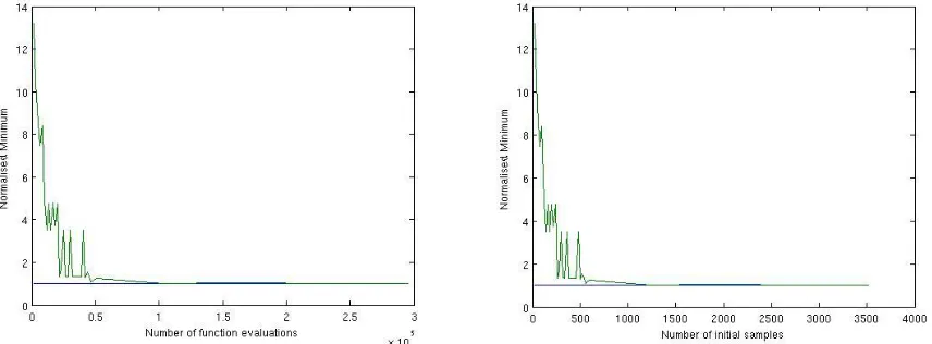
[image:10.612.87.515.377.535.2]The larger (the expected value of)N∗ is, the slower is the global convergence ofA. Figures 4a-b show the convergence profile for the bi-impulsive problem, 50 repeated independent runs Latin hypercube sampling, local optimization from each sample. Slightly more than 1000 initial samples are required to have a 100% convergence to the global minimum. However, the procedure in Algorithm 6 can be unpractical since, though
Figure 4. Convergence of a bi-impulsive direct transfer to Apophis as a function of the total number of function evaluations a) and number of initial samples b).
finite, the numberN∗ could be very large. In practice, what we would like is not to chooseN large enough so that a success is always guaranteed, but rather, for a fixed N value, we would like to maximize the probability of hitting a global minimizer. Now, let us define the following quantities:
δf(x) =|fglobal−f(x)|; δx(x) =∥xglobal−x∥ (19)
In case there is more than one global minimum point,δx(x) denotes the minimum distance betweenxand
all global minima. Moreover, in case the global minimum point xglobal is not known, we can substitute it
with the best known pointxbest. We can now define a new procedure, summarized in Algorithm 7. A key
Algorithm 7Convergence to the global optimum
1: set the max number of function evaluations for Aequal toN
2: applyA topforntimes
3: set j= 0
4: for alli∈[1, ..., n]do
5: ϕ(N, i) = minf(A(N), p, i)
6: x=arg ϕ(N, i)
7: computeδf(x) andδx(x)
8: if (δf(x)< tolf)∧(δx(x)< tolx)thenj =j+ 1 9: end if
10: end for
remain constant or should have a small variation. The choice of n will be discussed in Section IV.IV.A.2. Note that the values of the tolerance parameter tolf and tolx depend on the problem at hand. Algorithm
7 is applicable to general problems either presenting a single solution with value function fglobal (or fbest)
or presenting multiple solutions with valuefglobal (orfbest). On the other hand, in the following we are not
interested in distinguishing between solutions with equalf and differentxtherefore we will use a reduced version of Algorithm 7 in which the conditionδx(x)≤tolx is not considered.
Finally, we remark that the two procedures described in Algorithms 6 and 7 only consider the computational cost to evaluate f but not the intrinsic computational cost of A. The intrinsic cost of A is related to its complexity and to the number of pieces of informationAis handling. For instance, for a simple grid search such intrinsic cost is represented by the cost of sweeping through all the N points on the grid at which the objective function is evaluated. The intrinsic cost varies from algorithm to algorithm, but here we are assuming that the computational effort of the algorithms is dominated by function evaluations and, therefore, we do not take intrinsic costs into account.
IV.A. Performance Indexes
After the testing procedure has been defined, we move to the definition of performance indexes.
First we note that if the algorithmAis deterministic, then we can setn= 1. Indeed, each timeAis applied to p, it always returns the same value. Then, for deterministic algorithms, given a value N, a reasonable performance index is simplyJd(N) =ϕ(N,1), i.e. the best value returned by the algorithm.
Instead, for stochastic based algorithms different performance indexes can be defined. Such indexes are computed by running an algorithm over a problem a sufficiently high numbernof times. The indexes should reveal the ability of the algorithm to identify, in a given computational time (or computational effort), the best solution to a problem by running an algorithm a single time or, alternatively, by running it several times.
Possible indexes are the best, the mean and the variance of all the results returned by the n runs, or the probability of success of a single run. These will be discussed in what follows.
IV.A.1. Best, Mean and Variance
A common way to evaluate a stochastic algorithm is to collect the best value over a number of runs and to compute the mean and variance of the best values over the same number of runs. However, the use of best value, mean and variance presents some difficulties:
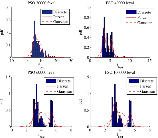
• The distribution of the best values is not Gaussian, as can be seen in Fig. 5 where the distribution of all the solutions found by PSO1009 over 200 runs for the EVM case is represented. Therefore the distance between the best and the mean values, or the value of the variance in general do not give an exact indication of the repeatability of the result. Moreover, it changes during the process, therefore we cannot define a priori the required number of runs to produce a correct estimation of mean and variance.
• The use of the best value could be misleading since. statistically, even a simple random sampling can converge to the global optimum. On the other hand an algorithm converging, on average, to a good value with a small variance does not guarantee that it will be able to find the best possible solution.
−100 0 10 20 30 0.1
0.2 0.3 0.4
fbest
PSO 20000 feval
Discrete Parzen Gaussian
0 5 10 15
0 0.2 0.4 0.6 0.8 1
fbest
PSO 40000 feval
Discrete Parzen Gaussian
0 2 4 6 8
0 0.5 1 1.5
fbest
PSO 60000 feval
Discrete Parzen Gaussian
0 2 4 6 8
0 0.5 1 1.5
fbest
PSO 100000 feval
[image:12.612.170.447.106.348.2]Discrete Parzen Gaussian
Figure 5. Probability density function for PSO applied to the solution of the EVM case: discrete, Gaussian (dashed) and kernel based approximation (continuous).
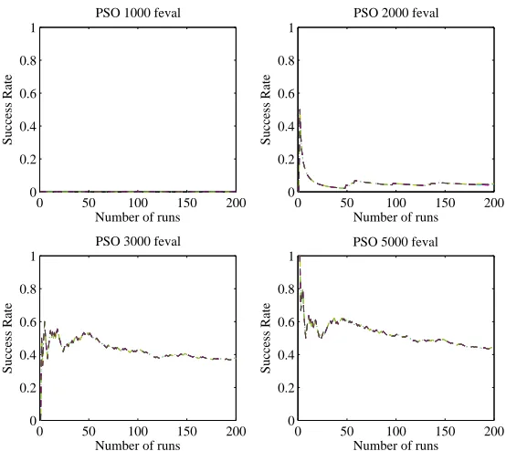
IV.A.2. Success Rate
An alternative index that can be used to assess the effectiveness of a stochastic algorithm is the success rate ps, which is related toj in Algorithm 7 byps =j/n. Considering the success as the referring index for a
comparative assessment implies two main advantages. First, it gives an immediate and unique indication of the algorithm effectiveness, addressing all the issues highlighted above, and, second, the success rate can be represented with a binomial probability density function (pdf), independent of the number of function evaluations, the problem and the type of optimization algorithm. This latter characteristic implies that the test can be designed fixing a priori the number of runs n, on the basis of the error we can accept on the estimation of the success rate. A usual starting point to determine the sample size for a binomial distribution is to assume that the sample proportion ps of successes (the success rate for a given nin our case) can be
approximated with a normal distribution, i.e. ps ∼ Np{θp, θp(1−θp)/n}, where θp is the unknown true
proportion of successes, and that the probability ofpsto be at distancederr fromθp,P r[|ps−θp| ≤derr|θp]
is at least 1−αb (see Ref.10). This leads to the expression:
n≥θp(1−θp)χ2(1),αb/d 2
err (20)
and to the conservative rule:
n≥0.25χ2(1),α
b/d 2
err (21)
obtained if θp = 0.5. For our tests we required an error ≤ 0.05 (derr = 0.05) with a 95% confidence
(αb = 0.05), which, according to Eq.(21), yieldsn≥176. This was extended to 200 for all the tests in this
paper in order to have a higher confidence in the result.
0 50 100 150 200 0
0.2 0.4 0.6 0.8 1
Number of runs
Success Rate
PSO 1000 feval
0 50 100 150 200
0 0.2 0.4 0.6 0.8 1
Number of runs
Success Rate
PSO 2000 feval
0 50 100 150 200
0 0.2 0.4 0.6 0.8 1
Number of runs
Success Rate
PSO 3000 feval
0 50 100 150 200
0 0.2 0.4 0.6 0.8 1
Number of runs
Success Rate
[image:13.612.167.444.54.301.2]PSO 5000 feval
Figure 6. The influence of sample size. The success rate is shown as function of the number of runs for the PSO applied to the solution of the bi-impulsive case.
IV.B. Test Results
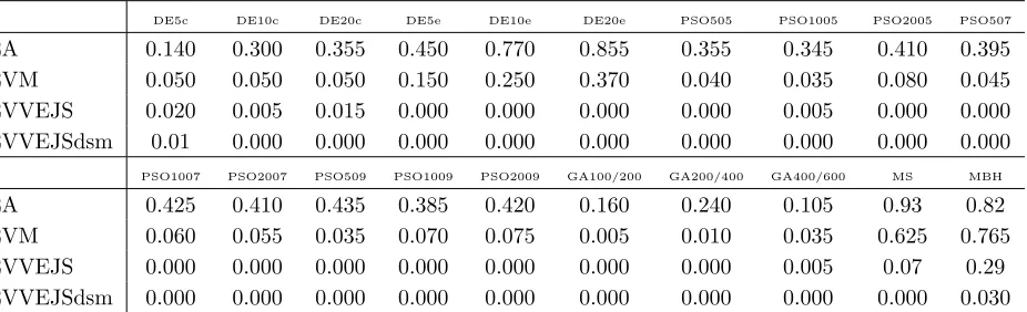
The results of the tests are summarized in Tables 1 and 2, where success probability (Table 1) and best value, mean and variance of best results (Table 2) are given for each of the 20 settings of the five stochastic solvers.
For both EA and EVM cases, success probability allows a fair classification and gives a clear indication of the best performing algorithms. If we look only at the set of evolutionary based algorithms (DE, GA and PSO), algorithms DE10e and DE20e perform undoubtedly better than the others and algorithms GA100/200-GA200/400-GA400/600 appear to be the worst performing ones. Algorithm DE5e wins a bronze medal, but if we can be confident in its third position for the EVM problem, we cannot have the same level of confidence regarding the third position for EA, because of the proximity of other algorithms. Actually, due to the binomial nature of the success and the adopted sample size, it is not possible to discriminate fairly between algorithms for which the success distance is smaller than the expected error (0.05 in our computations). Therefore, algorithm DE10e has to be considered at the same level as algorithms PSO1007, PSO509, for example, and other PSO settings. For the same reasons, we can say that, among the PSO settings, algorithms PSO1007 and PSO509 perform better than algorithm PSO1005 but the remaining PSO algorithms work at the same level.
An analogous vagueness is displayed by most of the evolutionary based algorithms when applied to EVM and almost all of them when applied to EVVEJS and EVVEJSdsm. On the other hand, MS and MBH shows remarkable performance in all the test cases with the simple MS winning over all the others in the EA case. For the EVVEJS case, all the algorithms but MBH appear practically unsuccessful, because, even if the success probability cannot be considered really 0 due to the error margin, it is≤0.12, according to the expected error. MBH is the only algorithm that can be practically used to solve this problem with a success
≤0.34. For EVVEJSdsm case even MBH is performing poorly, with a success≤0.08.
Table 1. Success for the 20 algorithms on the four test-cases. To compute the success, followingtolf values were used:
0.001 for EA,3−fbest for EVM,5−fbest for EVVEJS and8.5−fbestfor EVVEJSdsm
DE5c DE10c DE20c DE5e DE10e DE20e PSO505 PSO1005 PSO2005 PSO507
EA 0.140 0.300 0.355 0.450 0.770 0.855 0.355 0.345 0.410 0.395
EVM 0.050 0.050 0.050 0.150 0.250 0.370 0.040 0.035 0.080 0.045 EVVEJS 0.020 0.005 0.015 0.000 0.000 0.000 0.000 0.005 0.000 0.000 EVVEJSdsm 0.01 0.000 0.000 0.000 0.000 0.000 0.000 0.000 0.000 0.000
PSO1007 PSO2007 PSO509 PSO1009 PSO2009 GA100/200 GA200/400 GA400/600 MS MBH
EA 0.425 0.410 0.435 0.385 0.420 0.160 0.240 0.105 0.93 0.82
EVM 0.060 0.055 0.035 0.070 0.075 0.005 0.010 0.035 0.625 0.765 EVVEJS 0.000 0.000 0.000 0.000 0.000 0.000 0.000 0.005 0.07 0.29 EVVEJSdsm 0.000 0.000 0.000 0.000 0.000 0.000 0.000 0.000 0.000 0.030
global optimal solutions, algorithm PSO1009 is noticeably better: it is able to find the global solution, even if it is less robust and gets stuck many times in a far basin (see Figs. 5 and 7).
In order to solve an uncertainty condition, for instance when the success probability appears uniformly null, relaxing the tolf value could be useful. Focusing on the EVVEJS case, there is no way to correctly
discriminate among the algorithms on the basis of data in Table 1, but if the success threshold is raised from 5 to 5.3, then a superior performance of GAs is revealed. Most likely, this behavior is due to a combination of different features, such as larger population, the mutation search operator and a non-deterministic selection operator, which in this complex case reduces the speed of local convergence, preserves diversity and allows for a better exploration of the search space.
For the EVVEJSdsm case we are not so “lucky”. Raising the success threshold from 8.5 to 9 (see Table 3) identifies MBH as the only one algorithm practically able to handle this problem, but does not give any useful information to discriminate among the other algorithms. Only the DEc series and MS are able to find solutions with an objective value below 9, but the success rate is so low and similar that discriminating between the two would be difficult.
2 4 6 8
0 0.5 1 1.5 2 2.5
f
best
MPGA EVM 20000 feval
discrete parzen gaussian
2 3 4 5 6
0 1 2 3 4
f
best
.MPGA EVM 40000 feval
discrete parzen gaussian
2 3 4 5 6
0 1 2 3 4
f
best
MPGA EVM 60000 feval
discrete parzen gaussian
2 3 4 5 6
0 1 2 3 4 5
f
best
.MPGA EVM 100000 feval
discrete parzen gaussian
Figure 7. Pdfs, for the EVM case with the GA algorithm.
[image:14.612.78.541.77.218.2] [image:14.612.196.418.416.625.2]Table 2. Indexes: Best value, Mean Best, Variance Best.
EA (N=5000) EVM (N=100000) EVVEJS (N=400000) EVVEJSdsm (N=600000)
DE5c 4.37 4.7 0.07 2.98 3.6 0.32 4.93 12.51 15.07 8.42 16.37 11.93 DE10c 4.37 4.57 0.03 2.98 3.51 0.09 4.93 11.37 15.75 8.62 16.07 11.68 DE20c 4.37 4.52 0.02 2.98 3.43 0.08 4.93 9.97 15.93 8.7 16.02 20.33 DE5e 4.37 4.51 0.02 2.98 3.29 0.03 5.3 8.15 9.75 14.41 26.87 6.06 DE10e 4.37 4.42 0.01 2.98 3.23 0.03 5.3 6.39 5.01 21.91 28.72 2.6
DE20e 4.37 4.39 0 2.98 3.17 0.03 5.3 5.56 1.4 24.86 30.08 2.03
PSO505 4.37 4.51 0.01 2.98 3.82 0.68 5.03 12.68 16.49 12.42 23.13 8.52 PSO1005 4.37 4.51 0.01 2.98 3.78 0.63 4.96 11.97 18.7 12.48 23.32 10.46 PSO2005 4.37 4.5 0.01 2.98 3.65 0.52 5.3 11.19 17.92 15.32 23.74 6.67 PSO507 4.37 4.51 0.01 2.98 4.04 1.01 5.01 11.74 17.73 11.37 22.06 9.54 PSO1007 4.37 4.49 0.01 2.98 3.93 0.83 5.06 10.73 17.27 13.61 22.53 7.53 PSO2007 4.37 4.5 0.01 2.98 3.73 0.6 5.02 10.47 18.43 10.19 22.17 8.55 PSO509 4.37 4.5 0.01 2.98 4.22 1.06 5.25 11.83 21.71 11.83 22.08 8.83 PSO1009 4.37 4.55 0.37 2.98 3.97 0.87 5.02 10.56 18.43 12.13 22.09 9.86 PSO2009 4.37 4.5 0.01 2.98 3.81 0.75 5.03 10.53 15.13 12.08 22.07 8.59 GA200 4.37 4.57 0.03 2.99 3.78 0.24 5.16 10.65 15.19 9.65 19.98 13.53 GA400 4.37 4.5 0.01 2.99 3.54 0.14 5.02 8.31 9.91 9.1 18.6 13.35 GA600 4.37 4.45 0.01 2.98 3.45 0.1 4.98 6.98 6.68 10.74 18.36 10.91
MS 4.37 4.39 0 2.98 3.02 0 4.94 5.28 0.03 8.62 14.52 4.92
[image:15.612.77.540.67.367.2]MBH 4.37 4.41 0 2.98 3.01 0 4.93 5.19 0.39 8.41 12.64 9.74
Table 3. Successes for the 20 algorithms on the EVVEJSdsm test-case, with the threshold varying from8.5−fbest to 9.0−fbest
DE5c DE10c DE20c DE5e DE10e DE20e PSO505 PSO1005 PSO2005 PSO507
8.5−fbest 0.01 0 0 0 0 0 0 0 0 0
8.6−fbest 0.02 0 0 0 0 0 0 0 0 0
8.7−fbest 0.05 0.04 0 0 0 0 0 0 0 0
8.8−fbest 0.06 0.06 0.02 0 0 0 0 0 0 0
8.9−fbest 0.06 0.06 0.05 0 0 0 0 0 0 0
9.0−fbest 0.06 0.06 0.06 0 0 0 0 0 0 0
PSO1007 PSO2007 PSO509 PSO1009 PSO2009 GA100/200 GA200/400 GA300/600 MS MBH
8.5−fbest 0 0 0 0 0 0 0 0 0 0.03
8.6−fbest 0 0 0 0 0 0 0 0 0 0.07
8.7−fbest 0 0 0 0 0 0 0 0 0.02 0.15
8.8−fbest 0 0 0 0 0 0 0 0 0.02 0.19
8.9−fbest 0 0 0 0 0 0 0 0 0.02 0.22
9.0−fbest 0 0 0 0 0 0 0 0 0.02 0.23
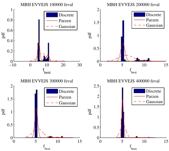
to a neighborhood of the best known solution as soon as the number of function evaluations increases. DE5c instead maintains a practically unchanged distribution of the solutions. In fact DE5c converges very fast and then tends to remain trapped in local minima.
Figs.12(a) to 13(b) represent the distribution of all the local minima in the search space, found by all the search algorithms over all the runs. In particular, we defined some specific intervals (or levels) of values for the objective function and then we computed: the average value of the relative distance of a given local minimum with respect to all the local minima in the same interval of objective values dil (or intra-level
[image:15.612.73.541.403.599.2]−100 0 10 20 30 0.2 0.4 0.6 0.8 1 f best pdf
MBH EVVEJS 100000 feval
Discrete Parzen Gaussian
0 5 10 15
0 0.5 1 1.5 2 f best pdf
MBH EVVEJS 200000 feval
Discrete Parzen Gaussian
0 5 10 15
0 0.5 1 1.5 2 f best pdf
MBH EVVEJS 300000 feval
Discrete Parzen Gaussian
0 5 10 15
0 0.5 1 1.5 2 2.5 f best pdf
MBH EVVEJS 400000 feval
Discrete Parzen Gaussian
Figure 8. Pdf for the MBH applied to the solution of the EVVEJS case with no DSMs.
0 50 100 150 200
0 0.2 0.4 0.6 0.8 1
Number of runs
Success Rate
100000 feval
0 50 100 150 200
0 0.2 0.4 0.6 0.8 1
Number of runs
Success Rate
200000 feval
0 50 100 150 200
0 0.2 0.4 0.6 0.8 1
Number of runs
Success Rate 300000 feval df 1.1df 1.2df 1.3df 1.4df 1.5df 1.6df
0 50 100 150 200
0 0.2 0.4 0.6 0.8 1
Number of runs
Success Rate
400000 feval
Figure 9. Success rate of the MBH applied to the solution of the EVVEJS case with no DSMs.
minima in the interval with lower values of the objective functiondtl (or trans-level distance). The figures
give an immediate representation of the diversity of the local minima in the search space (different colors correspond to different levels). Note that the two quantities dil and dtl can be related to the Shannon’s
diversity index.23 In fact, if both dtl and dil are large then the solutions belonging to each species (the
[image:16.612.168.446.53.302.2] [image:16.612.169.445.349.602.2]−200 0 20 40 0.1 0.2 0.3 0.4 fbest pdf
DE EVVEJS 100000 feval
Discrete Parzen Gaussian
−200 0 20 40
0.1 0.2 0.3 0.4 fbest pdf
DE EVVEJS 200000 feval Discrete Parzen Gaussian
−200 0 20 40
0.1 0.2 0.3 0.4 fbest pdf
DE EVVEJS 300000 feval
Discrete Parzen Gaussian
−200 0 20 40
0.1 0.2 0.3 0.4 fbest pdf
DE EVVEJS 400000 feval Discrete Parzen Gaussian
Figure 10. Pdf for the DE applied to the solution of the EVVEJS case with no DSMs.
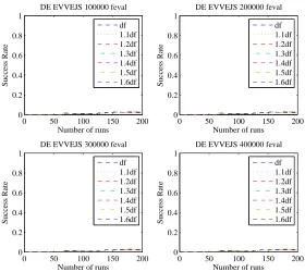
0 50 100 150 200
0 0.2 0.4 0.6 0.8 1
Number of runs
Success Rate
DE EVVEJS 100000 feval
df 1.1df 1.2df 1.3df 1.4df 1.5df 1.6df
0 50 100 150 200
0 0.2 0.4 0.6 0.8 1
Number of runs
Success Rate
DE EVVEJS 200000 feval
df 1.1df 1.2df 1.3df 1.4df 1.5df 1.6df
0 50 100 150 200
0 0.2 0.4 0.6 0.8 1
Number of runs
Success Rate
DE EVVEJS 300000 feval
df 1.1df 1.2df 1.3df 1.4df 1.5df 1.6df
0 50 100 150 200
0 0.2 0.4 0.6 0.8 1
Number of runs
Success Rate
DE EVVEJS 400000 feval
df 1.1df 1.2df 1.3df 1.4df 1.5df 1.6df
Figure 11. Success rate of the DE applied to the solution of the EVVEJS case with no DSMs.
each solution as a separate species the the value of the diversity index would be high. If both dtl anddil
are small the solutions are clustered and close to each other, therefore species are made of large groups of solutions and the diversity index would be low. The index would be low also fordilsmall anddtl large and
would be large for dil large and dtl small. It should be noted thatdtl and dil give a better representation
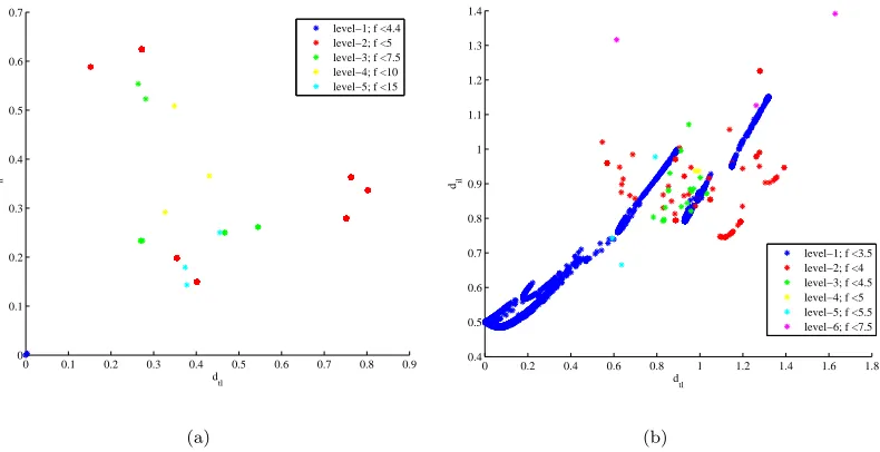
[image:17.612.167.448.51.300.2] [image:17.612.166.446.343.593.2]0 0.1 0.2 0.3 0.4 0.5 0.6 0.7 0.8 0.9 0
0.1 0.2 0.3 0.4 0.5 0.6 0.7
dtl
dil
level−1; f <4.4 level−2; f <5 level−3; f <7.5 level−4; f <10 level−5; f <15
(a)
0 0.2 0.4 0.6 0.8 1 1.2 1.4 1.6 1.8
0.4 0.5 0.6 0.7 0.8 0.9 1 1.1 1.2 1.3 1.4
dtl
dil
level−1; f <3.5 level−2; f <4 level−3; f <4.5 level−4; f <5 level−5; f <5.5 level−6; f <7.5
(b)
Figure 12. Relative distance of the local minima for a) the bi-impulsive and b) the EVM case.
0 0.2 0.4 0.6 0.8 1 1.2 1.4
0 0.5 1 1.5
dtl
dil
level−1; f <5 level−2; f <5.5 level−3; f <7.5 level−4; f <10 level−5; f <15 level−6; f <20
(a)
0 0.5 1 1.5 2 2.5
0.4 0.6 0.8 1 1.2 1.4 1.6 1.8 2 2.2 2.4
dtl
dil
level−1; f <8.6 level−2; f <9 level−3; f <9.5 level−4; f <10 level−5; f <15 level−6; f <20 level−7; f <25
(b)
Figure 13. Relative distance of the local minima for the EVVEJS: a) without DSM’s and b) with DSM’s.
More precisely, Fig.12(a) is telling us that for the bi-impulsive case the minima are quite spread, not clustered if not in pairs. The EVM case, in Fig.12(b), presents an almost continuous distribution of minima. However, the minima of one level appear to be quite distant from the minima of the lower level.
Fig.13(a) presents a quite different structure. There are a number of clusters and in particular three of them, corresponding to level 1,2 and 3, have values ofdtlanddillower than 0.2. The existence of clusters of minima
with lowdtl and lowdilsuggests an easy transition from one level to an another. An easy transition among
levels favors the search mechanism of MBH and represent a clue of a possible underlying funnel structure.20
Both Figs. 13(b) and (14) present a different distribution of the minima for the EVVEJSdsm case. The solutions are quite spread and with values of bothdtlanddilhigher than 0.5. This case appears to be highly
[image:18.612.113.508.64.267.2] [image:18.612.113.510.324.525.2]0 10 20 30 40 0
0.05 0.1 0.15 0.2
fbest
MBH EVVEJS−DSM 150000 feval discrete parzen gaussian
0 10 20 30
0 0.05 0.1 0.15 0.2 0.25
fbest
MBH EVVEJS−DSM 300000 feval discrete parzen gaussian
0 10 20 30
0 0.05 0.1 0.15 0.2 0.25
f
best
MBH EVVEJS−DSM 450000 feval discrete parzen gaussian
0 10 20 30
0 0.1 0.2 0.3 0.4
f
best
MBH EVVEJS−DSM 600000 feval discrete parzen gaussian
Figure 14. Examples of pdfs, for the EVVEJS case with DSM and the MBH optimizer.
still very high. Note that in the case of the EVVEJS problem with no deep-space manoeuvre running the MBH with no re-sampling provides an increase in performance from 29% to 37.5%.
Note that although the dtl −dil plots can provide clues on the characteristics of the search space, its
structure can be revealed only by an analysis of the actual position of all the local optima and not just by a measurement of their reciprocal distance. On the other hand, knowing all the local optima of a problem would mean having solved completely the problem. Therefore, thedtl−dilplane can be useful either to infer
from the characteristics of a benchmark test case the characteristics of other unsolved problems belonging to the same class (i.e. with an expected similar structure) or to devise the proper heuristics for solving a new problem when some local optima are already available.
V.
A Dynamical System Prospective
In this section we look at some evolutionary heuristics from a different prospective in the attempt to better understand the dynamics of the search process regardless of the problem under investigation. This analysis will be used to improve the performance of one of the algorithms tested above. In particular, we note that both DE and PSO can be rewritten in a compact form as a discrete dynamical system:
vi,k+1= (1−c)vi,k+ui,k
xi,k+1=xi,k+νS(xi,k+vi,k+1)vi,k+1
(22)
with
ν= min([vmax, vi,k+1])/vi,k+1 (23)
The controlui,kdefines the next point that will be sampled for each one of the existing points in the solution
space, the vectors xi,k and vi,k define the current state of a point in the solution space at stage k of the
search process and c is a viscosity, or dissipative coefficient, for the process. Eq. (23) represents a limit sphere around the pointxi,k at stagekof the search process.
In addition to Eq. (22) and Eq. (23), each optimization algorithm has heuristics responsible for selecting the new candidate points generated with ui,k. The selection operator is expressed through the function
S(xi,k+vi,k+1) which can be either 1 if the candidate point is accepted or 0 if it is not accepted.
Differential Evolution, in its basic form, has the ui,k defined by Eq.(13), viscosity c = 1 andvmax= +∞.
The selection function S can be either 1 or 0 depending on the relative value of the objective function of the new candidate individual generated with Eq.(13) with respect to the one of the current individual (see Algorithm 2). Particle swarm optimization has ui,k defined in Eq.(16) with the viscosity term c =
[image:19.612.197.418.52.251.2]constrained by Eq. (23). Note that if we take c2r2 = Fe, c1r1 = e and replacing xgi,k with one of the
individuals in the population, then PSO translates into DE and vice versa, we can go from DE to PSO just by properly defining the selection of the individualsxi1,k,xi2,k,xi3,k, the value of the coefficientsc, c1, c2, ν
and the selection functionS.
The discrete dynamical system in Eqs. (22) can be rewritten in matrix form as follows:
[ x
i,k+1 vi,k+1
]
=Ji,k
{ x
i,k
vi,k
}
(24)
and if we consider all the individuals in the population:
[ x
k+1
vk+1
]
=Jk
{ x
k
vk
}
(25)
The map (25) allows for a number of considerations on the evolution of the search process and therefore on the properties of the global optimization algorithm. In particular the map can:
• Diverge to infinity. In this case the discrete dynamical system is unstable, the global optimization algorithm is not convergent.
• Converge to a fixed point inD. In this case the global optimization algorithm is simply convergent in Dand we can define a stopping criterion. Once the search is stopped we can define a restart procedure. Depending on the convergence profile, the use of a restart procedure can be more or less efficient.
• Converge to a limit cycle in which the same points inDare re-sampled periodically. Even in this case we can define a stopping criterion and a restart procedure.
• Converge to a strange (chaotic) attractor. In this case a stopping criterion cannot be clearly defined because different points are sampled at different iterations.
We have seen in the previous sections that the heuristics implemented in MBH are particularly effective. MBH is based on a Newton (or quasi-Newton) method for local minimization and on a restart of the search within a neighborhoodNρ of a local minimum. We can view such local optimization methods asdynamical systemswhere the evolution of the systems at each iteration is controlled by some mapJk. Under suitable
assumptions, the systems converge to a fixed point. For instance, iff is convex andC2 in a small enough
domainDk containing a local minimum which satisfies some regularity conditions, Newton’s map converges
quadratically to a single fixed point (the local minimum) inDk.
The motivations for using different dynamical systems are: dropping the requirement for the continuity and differentiability of f; automatically reducing the size of the region in which a candidate point is generated (the basic version of MBH has a constant size of Nρ); and performing not only a local exploration of the
neighborhood, but also a global one. For instance, in the specific case of simple Differential Evolution,c= 1 andν = 1, therefore we have the reduced map:
xi,k+1=xi,k+S(xi,k+ui,k)ui,k (26)
or in matrix form for the entire populationxk+1=Jkxk. The interest is now in the properties of map (26).
We start by observing that ifS(xk+uk) = 1⇔f(xk+uk)< f(xk) the global minimizer xg∈D is a fixed
point for (26) since every pointx∈D is such thatf(x)> f(xg).
Then, let us assume that at every iterationkwe can find two connected subsetsDk andD∗k ofD such that
f(xk)< f(x∗k),∀xk∈Dk,∀xk∗ ∈Dk∗\Dk, and let us also assume thatPk ⊆Dk whilePk+1⊆D∗k(recall that
PkandPk+1 denote the populations at iterationkandk+ 1 respectively). Ifxlis the lowest local minimum
inDk, thenxlis a fixed point inDk for (26). In fact, every point generated by (26) (or (25)) must be inDk
andf(xl)< f(x),∀x∈Dk
Now we want to know if there are other fixed points for the dynamics (26) and if we can always have a simple convergence in Dk. First of all we note that if for every k, Pk ⊆Dk and Pk+1 ⊆D∗k, then the reciprocal
distance of the individuals cannot grow indefinitely because of the map (26), therefore the map cannot be divergent.
Then, if we assume that the functionf is strictly quasi-convex25inDk, we can prove that (26) converges to
Lemma V.1 If f is continuous and strictly quasi-convex on a compact set Dj, the following minimization problem withF ∈(0,1) has a strictly positive minimum valueδr(ϵ):
δr(ϵ) = min g(y1,y2) =f(y2)−f(Fy1+ (1−F)y2)
s.t. y1,y2∈Dk ∥y1−y2∥ ≥ϵ f(y1)≤f(y2)
(27)
Proof Since f is strictly quasi-convex g(y1, y2) > 0, ∀y1, y2 ∈ D; furthermore, the feasible region is
compact and, therefore, according to Weierstrass’ theorem the function g attains its minimum value over the feasible region. If we denote by (y∗1,y∗2) a global minimum point of the problem, then we have
δr(ϵ) =g(y1∗,y∗2)>0. (28)
Theorem V.2 Given a function f that is strictly quasi-convex overDk and a populationPk ∈Dk, then if
F ∈(0,1) and S(xk+uk) = 1⇔f(xk+uk)< f(xk) , the populationPk converges to a fixed point inDk fork→ ∞.
Proof We propose two distinct proofs for this result. The first one is simpler but requires an additional assumption. The second one is more complicated but also more general.
The first simpler proof requires the additional assumption that the population always has an individual xj,k that is strictly better than the others, i.e. f(xj,k)< f(xi,k) for anyi̸=j, then the map (26) at each
iterationkcan generate, with strictly positive probability, a displacement (xj,k−xi,k) for all the members
of the population. This means that at each iteration we have a strictly positive probability that the whole population collapses into a single point. Then, for k→ ∞the whole population collapses to a single point with probability one.
The more complicated and more general proof is the following. By contradiction let us assume that we do not have convergence to a fixed point. Then, it must hold that:
inf
k max{∥xi,k−xj,k∥, i, j∈[1, ..., npop]} ≥ϵ >0 (29)
At every generationk the map can generate with a strictly positive probability, a displacement F(xi∗,k−
xj∗,k), wherei∗andj∗identify the individuals with the maximal reciprocal distance, such that the candidate
point isxcand=Fxi∗,k+ (1−F)xj∗,kwithf(xi∗,k)≤f(xj∗,k). Since the functionf is strictly quasi-convex,
the candidate point is certainly better thanxj∗,k and, therefore, is accepted byS. Now, in view of (29) and
of Lemma (V.1) we must have that
f(xcand)≤f(xj,k)−δr(ϵ). (30)
Such reduction will occur with probability one infinitely often, and consequently the function value of at least one individual will be, with probability one, infinitely often reduced byδr(ϵ). But this way the value
of the objective function of such individual would diverge to −∞, which is a contradiction because f is bounded from below over the compact setDk.
In particular, the above result shows that, when the population of DE lies at each iteration in the neigh-borhood of a local minimum satisfying some regularity assumption (e.g., the Hessian at the local minimum is definite positive, implying strict convexity in the neighborhood), then DE will certainly converge to a fixed point. For general functions, we can not always guarantee that the population will converge to a fixed point, but we can show that the maximum difference between the objective function values in the population converges to 0, i.e. the points in the population tend to belong to the same level set.
Theorem V.3 Given a function f and a population Pk ∈Dk, then if F ∈ (0,1) and S(xk +uk) = 1 ⇔
f(xk+uk)< f(xk), the following holds
max
i,j∈[1,...,npop]
|f(xj,k)−f(xi,k)|→0,