Forecasting using Bayesian and information theoretic model averaging: an application to UK inflation

      

City, University of London Institutional Repository

Citation: Kapetanios, G., Labhard, V. and Price, S. (2007). Forecasting using Bayesian

and information theoretic model averaging: an application to UK inflation (07/15). London, UK: Department of Economics, City University London.

This is the unspecified version of the paper.

This version of the publication may differ from the final published

version.

Permanent repository link: http://openaccess.city.ac.uk/1476/

Link to published version: 07/15

Copyright and reuse: City Research Online aims to make research

outputs of City, University of London available to a wider audience.

Copyright and Moral Rights remain with the author(s) and/or copyright

holders. URLs from City Research Online may be freely distributed and

linked to.

City Research Online: http://openaccess.city.ac.uk/ [email protected]

Department of Economics

School of Social Sciences

Forecasting using Bayesian and information theoretic model

averaging: an application to UK inflation

George Kapetanios

1

Queen Mary University of London

Vincent Labhard

2

Bank of England

Simon Price

3

Bank of England and City University

Department of Economics

Discussion Paper Series

No. 07/15

1 _{Email: [email protected].}

2 _{Email: [email protected]}

3 Department of Economics, City University, Northampton Square, London, EC1V

Forecasting using Bayesian and

information theoretic model averaging:

an application to UK in ation

George Kapetanios

y

Queen Mary University of London

Vincent Labhard

z

Bank of England

Simon Price

x

Bank of England and City University

June 2006

Abstract

Model averaging often improves forecast accuracy over individual forecasts. It may also be seen as a means of forecasting in data-rich environments. Bayesian model av-eraging methods have been widely advocated, but a neglected frequentist approach is to use information theoretic based weights. We consider the use of information-theoretic model averaging in forecasting UK in ation, with a large data set, and

nd that it can be a powerful alternative to Bayesian averaging schemes.

Keywords: forecasting, in ation, Bayesian model averaging, Akaike criteria, forecast

combining

JEL: C110, C150, C530

This paper represents the views and analysis of the authors and should not be thought to represent those of the Bank of England or Monetary Policy Committee members. We are grateful for comments from two anonymous referees, the Editor and an Associate Editor of the JBES.

y_{[email protected].}

1

Introduction

A key metric of a satisfactory forecast is precision, often de ned in a root mean square

error sense, and techniques that can deliver this are highly desirable. Model averaging is

one such that often improves forecast accuracy over individual forecasts.

Another aspect of forecasting is appropriate methodology in data-rich environments, and

in recent years there has been increasing interest in forecasting methods that utilise large

datasets. There is an awareness that there is a huge quantity of information available in

the economic arena which might be valuable for forecasting, but standard econometric

techniques are not well suited to extract this in a useful form. This is not an issue of

mere academic interest. Lars Svensson described what central bankers do in practice in

Svensson (2004). `Large amounts of data about the state of the economy and the rest of

the world ... are collected, processed, and analyzed before each major decision.' In an

e ort to assist in this task, econometricians began assembling large macroeconomic data

sets and devising ways of forecasting with them: James Stock and Mark Watson (e.g.,

Stock and Watson (1999)) were in the vanguard of this campaign.

One popular methodolgy is forecast combination, where information in many forecasting

models, typically simple and incomplete, are combined in some manner. Stepping back,

forecast combination originated not in the large data set programme, but from

observa-tions by forecast practitioners that for whatever reasons, combining forecasts (initially

by simple averaging) produced a forecast superior to any element in the combined set.

This may seem odd, as if it were possible to identify the correctly speci ed model (and

the data generating process (DGP) is unchanging), then it might seem natural so to do,

although this is less obvious than it may seem. The true DGP may include very many

variables that make it infeasible to estimate, and there is a general bene t from parsimony

in forecasting. But the weight of evidence dating back to Bates and Granger (1969) and

Newbold and Granger (1974) reveals that combinations of forecasts often outperform

in-dividual forecasts. Recent surveys of forecast combination from a frequentist perspective

are to be found in Newbold and Harvey (2002) and Clements and Hendry (1998); see also

Clements and Hendry (2002). Models may be incomplete, in di erent ways; they employ

di erent information sets. Forecasts might be biased, and biases can o set each other.

be taken into account. Thus, combining misspeci ed models may, and often will, improve

the forecast.

An alternative way of looking at this problem is from a Bayesian perspective. Here it

is assumed that there is a distribution of models, thus delineating the concept of model

uncertainty quite precisely. The basic problem, that a chosen model is not necessarily the

correct one, can then be addressed in a variety of ways, one of which is Bayesian model

averaging. From this point of view, a chosen model is simply the one with the best

pos-terior odds; but pospos-terior odds can be formed for all models under consideration, thereby

suggesting a straightforward way of constructing model weights for forecast combinations.

This has been used in many recent applications; for example, forecasting US in ation in

Wright (2003a).

There is an analagous frequentist information theoretic approach. In this context,

infor-mation theory suggest ways of constructing model con dence sets. We use this term in

a broader sense than in the related literature of Hansen, Lunde, and Nason (2005) and

Kapetanios, Labhard, and Schleicher (2006). Given we have a set of models, we can

de-ne relative model likelihood. Model weights within this framework have been suggested

by Akaike (initially, Akaike (1978)). Such weights are easy to construct using standard

information criteria. Our purpose, then, is to consider this way of model averaging as an

alternative to Bayesian model averaging.

In this paper we develop the information-theoretic alternative to Bayesian model averaging

and assess the performance of these techniques by means of a Monte Carlo study. We

then compare their performance in forecasting UK in ation. For this, we use a UK

data set which emulates the data set in Stock and Watson (2002) (see Appendix.) Our

ndings support those of Wright (2003a), who concludes that Bayesian model averaging

can provide superior forecasts for US in ation, but we nd that the frequentist approach

2

Forecasting using Model Averaging

2.1

Bayesian Model Averaging

The idea behind forecasting using model averaging re ects the need to account for model

uncertainty in carrying out statistical analysis. From a Bayesian perspective, model

un-certainty is straightforward to handle using posterior model probabilities. See for example

Min and Zellner (1993), Koop and Potter (2003), Draper (1995a) and Wright (2003a,b).

Brie y, under Bayesian model averaging a researcher starts with a set of models which have

been singled out as useful representations of the data. We denote this set as_M=_fMigNi=1

where Mi is the i-th of the N models considered. The focus of interest is some quantity

of interest for the analysis, denoted by . This could be a parameter, or a forecast, such

as in ation hquarters ahead. The output of a Bayesian analysis is a probability

distribu-tion for given the set of models and the observed data at time t. Denote the relevant

information set at timet byDt, and the probability distribution aspr( jD;M). This is

given by

pr( _jDt;M) = N

X

i=1

pr( _jMi; Dt)pr(MijDt) (1)

where pr( _jMi; Dt) denotes the conditional probability distribution of given a model

Mi and the data Dt and pr(MijDt) denotes the conditional probability of the model

Mi being the true model given the data. Implementation requires two quantities to be

obtained at each point in time. First,pr( _jMi; Dt) which is easily obtained from standard

model speci c analysis. Second, the weights, pr(MijDt). The weights are formed as part

of a stochastic process where pr(MijDt) is obtained from pr(MijDt 1), the conditional

probability of the model Mi being true, given the previous period's data. This requires

prior distributions forpr(MijD0) = pr(Mi) and pr( ijMi; Dt 1) to be speci ed.

Thus we need to obtain a number of expressions for (1) to be operational. First, using

Bayes' theorem

pr(MijDt) =

pr(DtjMi; Dt 1)pr(MijDt 1)

pr(DtjDt 1)

= _PNpr(DtjMi; Dt 1)pr(MijDt 1)

i=1pr(DtjMi; Dt 1)pr(MijDt 1)

(2)

where pr(DtjMi; Dt 1) denotes the conditional probability distribution of the data given

the modelMi and the previous period's data and

pr(DtjMi; Dt 1) = Z

is the likelihood of model Mi, where i are the parameters of model Mi. Given this, the

quantity of interest is

E( _jDt) = N

X

i=1

^

ipr(MijDt) (4)

In theory (see e.g. Madigan and Raftery (1994)) when is a forecast, this sort of

averaging provides better average predictive ability than single model forecasts.

2.2

Information Theoretic Model Averaging

In the context of non-Bayesian methods of forecasting the idea of model averaging (i.e.,

forecast combination) has a long tradition starting with Bates and Granger (1969). The

aim is to use forecasts obtained during some forecast evaluation period to determine

optimal weights from which a forecast can be constructed along the lines of (4). These

weights are usually constructed using some regression method and the available forecasts.

But a problem arises if N is large. For example, N=93 as in Wright (2003a) requires an

infeasibly large forecast evaluation period.

Although the literature on model averaging inference is dominated by work with Bayesian

foundations, there has also been some research based on frequentist considerations. Hjort

and Claeskens (2003) provide a brief overview in the context of analysing model

aver-aging estimators from a likelihood perspective. Most frequentist work focuses on the

construction of distributions and con dence intervals for estimators of parameters that

take into account, in some way, model uncertainty. Examples include Hurvich and Tsai

(1990), Draper (1995b), Kabaila (1995), P•otscher (1991), Leeband and P•otscher (2000)

and Kapetanios (2001). The work of Burnham and Anderson (1998), on which we build,

forms a substantial part of the frequentist model averaging work available in the

litera-ture. But the present paper is one of the rst to focus on forecasting as opposed to the

construction of con dence intervals in the context of frequentist model averaging.

Our alternative to Bayesian model averagaing is based on the analogue of pr(MijDt) for

frequentist statistics. Such a weight scheme has been implied in a series of papers by

Akaike and others (see, e.g., Akaike (1978, 1981, 1983, 1979) and Bozdogan (1987)) and

expounded further by Burnham and Anderson (1998). Akaike's suggestion derives from

the Akaike information criterion (AIC). AIC is an asymptotically unbiased measure of

parameters in the model, which may be viewed as a penalty for over-parameterization.

Akaike's original frequentist interpretation relates to the classic mean-variance trade-o ,

although Akaike (1979) o ers a Bayesian interpretation. In nite samples, when we add

parameters there is a bene t (lower bias), but also a cost (increased variance). More

technically, from an information theoretic point of view,AIC is an unbiased estimator of

the Kullback and Leibler (1951) (KL) distance of a given model where the KL distance

is given by

I(f; g) =

Z

f(x) log f(x)

g(x_j ) dx:

Heref(x) is the unknown true model generating the data,g(x_j:) is the entertained model

and is the probability limit of the parameter vector estimate for g(x_j:). I(f; g) is not

known. It can be replaced by

^

I(f; g) =

Z

f(x) log f(x) g(x_j^)

!

dx:

where ^ is the estimator of the parameter vector . However, ^I(f; g) cannot be used either

asf(x) is not known. Using an observed sample x1; : : : ; xT, ^I(f; g) can be approximated

by

~

I(f; g)1 T

T

X

t=1

logf(xt)

1 T

T

X

t=1

logg(xij^)

The rst term of ~I(f; g) is still unknown, but it remains constant when comparing di erent

models g and so is an operational model selection criterion. However, although ~I(f; g)

and ^I(f; g) have the same probability limit, the mean of the asymptotic distribution of

T( ~I(f; g)- ^I(f; g)) is not zero. Akaike's main contribution is to derive an expression for this

bias under certain regularity conditions. In particular, Akaike showed that the asymptotic

expectation of T( ~I(f; g)- ^I(f; g)) is p where p is the dimension of . More details on the

derivation of this asymptotic expectation may be found in, e.g., Gourieroux and Monfort

(1995, pp. 308-309).

So the di erence of the AIC for two di erent models can be given a precise meaning.

It is an estimate of the di erence between the KL distance for the two models. Further,

exp( 1=2 i) is the relative likelihood of modeliwhere i =AICi minjAICj andAICi

denotes the AIC of the ith model in _M. Thus exp( 1=2 i) can be thought of as the

odds for the ith model to be the best KL distance model in _M. So this quantity can be

viewed as the weight of evidence for model ito be the KL best model given that there is

do not require the assumption that the true model belongs to_M. We are only considering

the ranking of models in terms of KL distance. It is natural to normalise exp( 1=2 i)

so that

wi =

exp( 1=2 i)

PN

i=1exp( 1=2 i)

(5)

where P_iwi = 1. We refer to these as AIC weights. As the Akaike criterion is only

one of several criteria which can form the basis of such weights, we also consider weights

based on the Schwartz information criterion (SIC), which has a similar rationale. We

consider both versions of the information-theoretic model averaging (ITMA)approach in

the exercises we report below: one based on AIC weights (AITMA), and another based

on SIC weights (SITMA).

We note wi are not the relative frequencies with which given models would be picked up

according to AIC as the best model given _M. Since the likelihood provides a superior

measure of data based weight of evidence about parameter values compared to such

rela-tive frequencies (see, e.g., Royall (1997)), it is reasonable to suggest that this superiority

extends to evidence about a best model given _M. In Bayesian language, the wi might

be thought of as model probabilities under noninformative priors. However, this

anal-ogy should not be taken literally as these model weights are rmly based on frequentist

ideas and do not make explicit reference to prior probability distributions about either

parameters or models.

3

Monte Carlo evidence

We now undertake a small Monte Carlo study to explore the properties of various model

averaging techniques in the context of forecasting. As we discussed above, model averaging

aims to address the problem of model uncertainty in small samples. There are two broad

cases that may be considered. The rst is when the model that generates the data belongs

to the class under consideration. In this case it addresses the issue that the chosen model is

not necessarily the true model, and by assigning probabilities to various models provides

a forecast that is, to some extent, robust to model uncertainty. The second, perhaps

more relevant case, is where the true model does not belong to the class of models being

considered. Here there is no possibility that the chosen model will capture all the features

since forecasts from di erent models can inform the overall forecast in di erent ways. We

examine this latter case.

In the experimental design, we adapt the setup proposed in Fernandez, Ley, and Steel

(2001) and subsequently used repeatedly, for example in Eklund and Karlsson (2005). It

therefore o ers a standard problem to examine. LetX= (x1; : : : ; xN) be a T N matrix

of regressors, where xi = (xi;1; : : : ; xi;T)0. The series in the rst 2N=3 columns are given

by

xi;t = ixi;t 1+ i;t; i= 1; : : : ; N; t= 1; : : : ; T (6)

where t is i.i.d. N(0;1). The last N=3 series are constructed as

(x2N=3+1; : : : ; xN) = (x1; : : : ; xN=3)(0:3; : : : ;0:3 + (N=3 1)0:2)0(1; : : : ;1) +E (7)

where E is a T N=3 matrix of standard normal variates. This setup allows for some

cross sectional correlation in the predictor variables. The true model is given by

yt= 2x1;t x5;t+ 1:5x7;t+x11;t+ 0:5x13;t+ 2:5"t (8)

where "t is i.i.d. N(0;1). The numbering of the variables is prompted partly by the size

of the data set and features of the models investigated in the source references, but this

is not a critical feature of the design. The important point is that none of the models

considered are the true DGP.

The design in Eklund and Karlsson (2005) sets N = 15 and i = 0. We generalise it

in two directions. First, we set N = 60, the nearest round number to our own dataset.

Second, we let i U(0:5;1). The i introduce persistence, which we allow to be random.

The benchmark is the forecast produced by a simpleAR(1) model foryt. For the remaining

forecasts, we use the model

yt+h =a0xt+byt+"t (9)

for theh-step ahead forecast, wherext is aK-dimensional regressor set, and K takes the

value of 1 or 2. As K is no greater than 2, the true model can never be selected.

The combinations we evaluate are based on the complete set of models of form (9). The

rst three combinations are produced by Bayesian Model Averaging (BMA), which in

some sense are benchmarks given their wide adoption, di ering by a shrinkage parameter

we set the model prior probabilitiesP(Mi) to the uninformative priors 1=N. The prior for

the regression coe cients is chosen to be given byN(0; 2_(X0_X) 1_{), conditional on} 2_,

whereX is theT pregressor matrix for a given model andpis the numbers of regressors.

We assume strict exogeneity of the X. The improper prior for 2 is proportional to 1= 2.

The speci cation for the prior of the regression coe cients implies a degree of shrinkage

towards zero (which implies no predictability). The degree of shrinkage is controlled by .

The rationale is that some degree of shrinkage steers away from models that may t well

in sample (by chance, or because of over tting) but have little forecasting power. There

is empirical evidence that such shrinkage is bene cial for out-of-sample forecasting, but

no a priori guidance for what values should be selected. Following Wright (2003a) we

consider conventional choices of = 20;2;0:5. Given the above, routine integration gives

model weights which are proportional to

(1 + ) p=2S (T+1) (10)

where

S2 =Y0Y Y0X(X0X) 1X0Y

1 + (11)

and Y is the T 1 regressand vector.

We next consider the ITMA weights introduced above, namely AITM and SITMa. Finally,

we examine equal-weight model averaging (AV) where the weights are given by 1=N. This

last scheme, employed for example in Stock and Watson (2004) (see also Stock and Watson

(2003)), is commonly used and often thought to work well in practice.

We setT = 50;100. The forecast evaluation period for each sample is the last 30

observa-tions. We examine the forecast horizons h= 1; : : : ;8. For all model averaging techniques

we consider two di erent classes of models over which the weighting scheme is applied.

The rst is all models with one predictor variables (K = 1), and the second all models

with two predictor variables (K = 2), neither of which contains the true model. We do

not allow for higher K for two reasons. First, most forecasting models used in practice,

and found to have good performance, are parsimonious. Second, weights are assigned

to all members of the model class. With our setup and K = 2 we have 1770 models to

consider. For (say) K = 3 the number of models rises to 34220 and therefore becomes

computationally intensive. Methods to search the model space e ciently do exist that

bypass this problem. One is that discussed by Fernandez, Ley, and Steel (2001) and

uses genetic and simulated annealing algorithms to search for good models in terms of

information criteria. But we do not explore these methods in this paper.

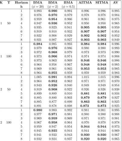
Results for forecast performance in terms of RMSE relative to the benchmark are given

in Table 1. The best forecast method in a particular row (that is, for given K, T and

h) are indicated in bold. These are evaluated to three decimal places, so in some cases

more than one model is `best', although at higher levels of numerical precision there is

always a single best performer. Variations in performance are reasonably large. It is

immediately evident that for this design the simple AR(1) benchmark does not perform

well, being dominated for most combinations of K, T and h by the combined forecasts.

Using simple averaging does better than the AR but is never best. In the Bayesian cases,

the low shrinkage parameter tends to do worst. A high shrinkage parameter improves

performance, but performance is best for the intermediate value. It is best in 16 out of

32 cases, especially for short horizons. The average value of the RRMSE is 0.942.

Our main interest is in the the information-criteria based methods. The two methods

(AITMA and SITMA) are based on penalty factors that are numerically similar in this

experiment, and the results are correspondingly close. As can be seen, they do well,

especially at longer horizons, where they tend to dominate BMA. Both AITMA and

SITMA and have the best forecast in 15 out of 32 cases, only one less than for the

intermediate BMA; similarly, the average RRMSE is a mere 0.003 greater at 0.945. The

equivalent performance is a robust result across samples and choice of K. Essentially,

it is hard to choose between the intermediate BMA and the information theoretic based

methods. In the remainder of the paper we see whether these conclusions carry over to

the real data.

4

Evidence from in ation forecasts

Our primary focus in this paper is practical, and in particular on the practice of in ation

forecasting using the model averaging schemes examined in the Monte Carlo study. The

models we consider are a standard speci cation, as discussed in Stock and Watson (2004).

We modify our Monte Carlo design by using a k1 lags autoregressive process augmented

with a k2 distributed lag on a single predictor variable. The number of lags in the pair

(k;1) where k is chosen optimally for each model, each sample and each forecast horizon

using the Akaike information criterion: we refer to these models as ARX(k).

Conse-quently, the lag structure for each predictor-variable model may vary with the horizon.

Thus, model ifor forecasting horizon h is given by

t+h = +

k1

X

j=1

j t j+1+ k2

X

j=1

xit j+1+ t (12)

where t is UK year-on-year CPI in ation, xit is the i-th predictor variable at timet and

t is the error term, with variance 2. As for the Monte Carlo experiment, the errors will

exhibit a M A(h 1) process. We consider 58 predictor variables, where the data span

1980Q2-2004Q1. We further include the AR forecast, making a total of 59 forecasts to

combine. Alongside the information theoretic combinations (based alternatively on AIC

and SIC as in the Monte Carlo exercise) we consider Bayesian and equal-weight model

averaging. The information theoretic weights are given by (5). The Bayesian weights are

given by the scheme discussed in the Monte Carlo section using (10) and (11).

We use data from the period 1980Q2 to 1990Q1. We evaluate the forecasts over two

post-sample periods: 1990Q2-1997Q1 (pre-MPC) and 1997Q2-2004Q1 (MPC). These are

natural dates to choose, as from May 1997 monetary policy was set by the Bank of

England's Monetary Policy Committee under an in ation targeting regime. Here we

focus on an evaluation in terms of a RMSE criterion; in the working paper version of this

paper Kapetanios, Labhard, and Price (2005) we also evaluate the combinations in terms

of forecast densities. We consider horizons up to three years (that is, h= 1; : : : ;12).

The forecasts are generated using a recursive forecasting scheme. For example, for the

rst evaluation period models are estimated up to 1990Q1 and 12 forecasts constructed

(that is, for each period between 1990Q2 and 1993Q1). Then the models are re-estimated

over the period 1980Q2 to 1990Q2 and forecasts constructed for the next 12 periods

as before. This is repeated for all the possible forecasts within the evaluation period.

From each re-estimation, the estimated log-likelihood is used to construct the relevant

information criterion which is in turn used to construct the information theoretic weights,

and similarly for the Bayesian weights. We report performance in terms of relative RMSE,

compared to the benchmark AR model, as well as two other indicators: the percentage

of models of the form (12) which perform worse than a given model averaging scheme

in terms of relative RMSE; and the proportion of periods in which the model averaging

three indicators are ranked similarly so we discuss only those from the rst. In the relative

RMSE tables we report a Diebold-Mariano (DM) test (Diebold and Mariano (1995)) of

whether the forecast is signi cantly di erent from the benchmark AR model at the 10%

level, indicated with an asterisc.

It is well known that the asymptotic distribution of the DM test statistic under the null

hypothesis of equal predictive ability for the two forecasts is not normal when the models

used to produce the forecasts are nested. A number of solutions have been proposed

for this problem: see Corradi and Swanson (2006) for a survey. We use the parametric

bootstrap to obtain the necessary critical values. An earlier example of the use of the

bootstrap for the Diebold Mariano test statistic is Killian (1999). Our bootstrap design

is straightforward. Under the null hypothesis the model generating the data is anAR(p)

model. We use the parametric bootstrap to construct bootstrap samples for in ation

from the recursively estimated AR(p) model. These bootstrap series are then combined

with the predictor variables, which are kept xed in the boostrap sample. Forecasts

are recursively produced for all the models and model averaging methods considered in

the forecasting exercise, in exactly the same way as the original forecasts. Then DM

statistics are produced and stored for every bootstrap replication. These statistics form

the empirical distribution from which the bootstrap critical values are obtained. 199

bootstrap replications are used.

We rst consider the MPC forecast evaluation period (Tables 2-4). The Akaike

informa-tion theory based AITMA beats the AR benchmark at all horizons. This is also true for

the simple average AV, but AITMA provides the best forecast in 8 out of 12 cases while

the AV provides none. In the table, `best' is de ned to three decimal places, so more

than one model can be `best'. In several cases the AIC and SIC are numerically identical

to three decimal places, but AITMA is absolutely best in all eight cases. The di erence

from the AR benchmark is signi cant in six of the eight cases. This is a strong result,

as forecast predictive tests have notoriously low power: Ashley (1998) concludes that `a

model which cannot provide at least a 30% MSE improvement over that of a competing

model is not likely to appear signi cantly better than its competitor over post sample

periods of reasonable size.' Moreover, AITMA beats the benchmark by a large margin

in many cases - with a RMSE advantage of over 5% in all cases, of 20% or more in eight

cases, and more than 30% in three cases. It does particularly well at long horizons,

this sample and this data set. The Bayesian BMA scheme works best for intermediate

in terms of the individual best forecast, but high (giving the data a high weight) is the

best Bayesian scheme overall, although clearly inferior to AITMA; and even the low

scheme is close to dominating the simple averaging scheme AV (which amounts to setting

= 0).

In the working paper version of this paper we report the top-ten ranked models for the

Bayesian and information theoretic schemes over the same period. The higher is , the

more weight is put on the variables with the highest in-sample explanatory power.

Com-paring the high and information theoretic schemes, the variables selected and weights

are very similar. However, the latter two give a little more weight to the best performer,

and the subsequent weights decline at a slower rate relative to the Bayesian scheme. The

AITMA and SITMA rankings are not identical but are extremely similar. Although there

is clearly a concentrated peak on the most important variable, in each combination all

the models enter with a non-zero weight; in that sense, the information in the entire data

set is being combined, although by the tenth variable the weight in both the SITMA and

the BMA with the highest are down to 0.5%.

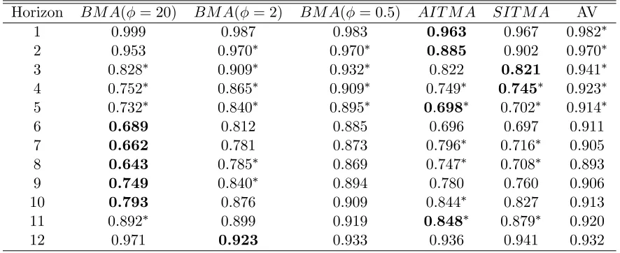
The conclusions remain broadly the same in the pre-MPC forecast evaluation period

(Tables 5-7), although the AITMA is no longer so clearly dominant. The best-performing

Bayesian ( = 20) combination provides best forecasts at ve horizons, compared to a

score of the four best for AITMA. Six of the AITMA forecasts are signi cantly better

than the benchmark: four of the Bayesian. In this period, while the AITMA continues

to place more weight on fewer variables, the weights are much less concentrated than in

the previous case. The variables selected by the high BMA and AITMA are now less

similar, but there is a high degree of commonality (as there is between the two samples).

Conceptually and practically, the two forecast combination methods are similar; as

men-tioned above, the model weights are not identical but there is a high degree of

com-monality. In both cases information is being gleaned from the data in-sample and used

to inform the forecast method. In the low-shrinkage case, the frequentist analogy is to

the likelihood-weighted scheme. As usual, the information theoretic measures steer away

from the raw likelihood with a parameter penalty, which can be seen as similar to the way

information criteria avoid over tting in standard model selection. It is well known that

information criteria can be given a Bayesian interpretation: see the discussion in Kadane

approx-imation to the Bayes factor to perform systematically better or worse than any other; all

we can conclude is that in these samples and data the AITMA performs comparably to the

Bayesian method. And unlike the Bayesian averaging, there is no requirement to select a

particular value for a key parameter ( ). Although we have not explored it in this paper,

in related work (Kapetanios, Labhard, and Price (2006)) we have extended the approach

to use information theoretic weights constructed with the predictive likelihood, which is

also a good performer. Finally, we note that although we nd these information-theoretic

techniques work well, and consider them a useful alternative to other techniques, we

nat-urally do not suggest that they would or should be used as the main or only forecasting

tool by any central bank.

5

Conclusions

Model averaging provides a well-established means of improving forecast performance

which works well in practice and has sound theoretical foundations. It may also be helpful

for another reason. In particular, in recent years there has been a rapid growth of interest

in forecasting methods that utilise large datasets, driven partly by the recognition that

policymaking institutions process large quantities of information, which might be helpful

in the construction of forecasts. Standard econometric methods are not well suited to this

task, but model averaging can help here as well.

In this paper we consider two averaging schemes. The rst is Bayesian model averaging.

This has been used in a variety of forecasting applications with encouraging results. The

second is an information theoretic scheme which we derive in this paper using the concept

of relative model likelihood developed by Akaike. Although the information theoretic

approach has received less attention than Bayesian model averaging, the evidence we

produce from a Monte Carlo study and an application forecasting UK in ation indicate

that it has at least some potential to produce more precise forecasts and therefore might

be a useful complement to other forecasting techniques. There are some advantages

in practice. In the frequentist approach the weights are straightforward to compute,

and there is less need to make arbitrary assumptions, for example about the shrinkage

parameter or the prior distribution.

on model performance, it would be odd if the alternative scheme were not also useful.

But our work shows that it may outperform Bayesian weights in some cases. Moreover,

it has a clear frequentist interpretation and is easy to implement with little judgement

required about ancillary assumptions. While it is highly unlikely that a single technique

would be more useful that all others in all settings, our work indicates that information

theoretic model averaging may provide a useful addition to the forecasting toolbox.

References

Akaike, H. (1978): \A Bayesian Analysis of the Minimum AIC Procedure," Annals of

the Institute of Statistical Mathematics, 30, 9{14.

(1979): \A Bayesian Extension of the Minimum AIC Procedure of Autoregressive

Model Fitting,"Biometrika, 66, 237{242.

(1981): \Modern Development of Statistical Methods," in Trends and progress

in system identi cation, ed. by P. Eykho , pp. 169{84. Pergamon Press Paris.

(1983): \Information Measures and Model Selection," International Statistical

Institute, 44, 277{291.

Ashley, R.(1998): \A New Technique for Postsample Model Selection and Validation,"

Journal of Economic Dynamics and Control, 22, 647{65.

Bates, J. M., and C. W. J. Granger (1969): \The Combination of Forecasts,"

Operations Research Quarterly, 20, 451{68.

Bozdogan, H.(1987): \Model Selection and Akaike's Information Criterion (AIC): the

General Theory and its Analytical Extensions," Psychometrika, 52(3), 345{70.

Burnham, K. P., and D. R. Anderson(1998): Model Selection and Inference. Berlin:

Springer Verlag.

Clements, M. P., and D. F. Hendry (1998): Forecasting Economic Time Series.

Cambridge: CUP.

Corradi, V., and N. R. Swanson(2006): \Predictive Density Evaluation," in

Hand-book of Economic Forecasting, ed. by C. W. J. G. G. Elliot, and A. Timmerman, pp.

197{284. (Amsterdam: Elsevier).

Diebold, F. X., and R. S. Mariano(1995): \Comparing Predictive Accuracy,"

Jour-nal of Business and Economic Statistics, 13, 253{63.

Draper, D. (1995a): \Assessment and propagation of model uncertainty," Journal of

the Royal Statistical Society Series B, 57, 45{97.

Draper, D. (1995b): \Assessment and propagation of model uncertainty," Journal of

the Royal Statistical Society, Series B, 57, 45{97.

Eklund, J., and S. Karlsson (2005): \Forecast Combination and Model Averaging

Using Predictive Measures,"CEPR Working Paper No. 5268.

Fernandez, C., E. Ley, and M. F. Steel (2001): \Benchmark Priors for Bayesian

Model Averaging,"Journal of Econometrics, 100, 381{427.

Gourieroux, C., and A. Monfort (1995): Statistics and Econometric Models:

Vol-ume 2. Cambridge: Cambridge University Press.

Hansen, P. R., A. Lunde, and J. M. Nason (2005): \Model Con dence Sets for

Forecasting Models," Working Paper 2005-7, Federal Reserve Bank of Atlanta.

Hjort, N. L., and G. Claeskens (2003): \Frequentist model average estimators,"

Journal of the American Statistical Association, 98, 879{99.

Hurvich, C. M., and C.-L. Tsai(1990): \The impact of model selection on inference

in linear regression," The American Statistician, 44, 214{17.

Kabaila, P. (1995): Econometric Theory11, 537.

Kadane, J. B., and N. Lazar (2004): \Methods and Criteria for Model Selection,"

Journal of the American Staistical Association, 99, 279{90.

Kapetanios, G. (2001): \Incorporating lag order selection uncertainty in parameter

inference for AR models," Economics Letters, 72, 137{44.

Kapetanios, G.(2005): \Variable Selection Using Non-Standard Optimisation of

Kapetanios, G., V. Labhard, and S. Price (2005): \Forecasting using Bayesian

and information theoretic model averaging: an application to UK in ation," Bank of

England Working Paper No. 268.

(2006): \Forecasting Using Predictive Likelihood Model Averaging,"Economics

Letters, 91, 373{79.

Kapetanios, G., V. Labhard, and C. Schleicher (2006): \Conditional Model

Con dence Sets with an Application to Forecasting Models," Manuscript, Bank of

England.

Killian, L.(1999): \Exchange Rates and Monetary Fundamentals: What Do We Learn

from Long-Horizon Regressions?,"Journal of Applied Econometrics, 14, 491.

Koop, G., and S. Potter(2003): \Forecasting in Large Macroeconomic Panels Using

Bayesian Model Averaging," Federal Reserve Bank of New York Report 163.

Kullback, S., and R. A. Leibler (1951): \On Information and Su ciency," Annals

of Mathematical Statistics, 22, 79{86.

Leeband, H., and B. M. P•otscher(2000): \The Finite-Sample Distribution of

Post-Model-Selection Estimators, and Uniform Versus Non-Uniform Approximations,"

Tech-nical Report TR 2000-03, Institut f•ur Statistik und Decision Support Systems,

Univer-sit•at Wien.

Madigan, D., and A. E. Raftery(1994): \Model Selection and Accounting for Model

Uncertainty in Graphical Models using Occam's Window," Journal of the American

Statistical Association, 89, 1,535{46.

Min, C., and A. Zellner(1993): \Bayesian and Non-Bayesian Methods for Combining

Models and Forecasts with Applications to Forecasting International Growth Rates,"

Journal of Econometrics, 56, 89{118.

Newbold, P., and C. W. J. Granger (1974): \Experience with Forecasting

Univari-ate Time Series and the Combination of Forecasts," Journal of the Royal Statistical

Society, Series A, 137, 131{65.

Newbold, P., and D. I. Harvey (2002): \Forecast Combination and Encompassing,"

in A Companion to Economic Forecasting, ed. by M. Clements, and D. F. Hendry,

P•otscher, B. M. (1991): \E ects of Model Selection on Inference,"Econometric

The-ory, 7, 163{85.

Royall, R. M. (1997): Statistical Evidence: a Likelihood Paradigm. New York:

Chap-man and Hall.

Stock, J. H., and M. W. Watson(1999): \Forecasting In ation," Journal of

Mone-tary Economics, 44, 293{335.

Stock, J. H., and M. W. Watson(2002): \Macroeconomic Forecasting Using Di

u-sion Indices," Journal of Business and Economic Statistics, 20, 147{62.

(2003): \Forecasting Output and In ation: the Role of Asset Prices," Journal

of Economic Literature, 41, 788{829.

(2004): \Combination Forecasts of Output Growth in a Seven Country Dataset,"

Journal of Forecasting, 23, 405{30.

Svensson, L. E. O. (2004): \Monetary Policy with Judgment: forecast Targeting,"

unpublished.

Wright, J. H. (2003a): \Bayesian Model Averaging and Exchange Rate Forecasts,"

Board of Governors of the Federal Reserve System, International Finance Discussion

Papers No 779.

(2003b): \Forecasting US In ation by Bayesian Model Averaging," Board of

Governors of the Federal Reserve System, International Finance Discussion Papers No

[image:21.612.79.482.163.627.2]

Table 1: Monte Carlo Study: RMSE of various Model Averaging schemes

K T Horizon BMA BMA BMA AITMA SITMA AV

h ( = 20) ( = 2) ( = 0:5)

1 0.993 0.990 0.994 0.996 0.996 0.995

2 0.976 0.970 0.979 0.978 0.978 0.984

3 0.959 0.954 0.966 0.961 0.961 0.975

1 50 4 0.947 0.936 0.952 0.950 0.950 0.965

5 0.935 0.923 0.941 0.905 0.905 0.959

6 0.919 0.910 0.932 0.907 0.907 0.954

7 0.922 0.908 0.929 0.902 0.902 0.952

8 0.921 0.907 0.927 0.903 0.903 0.949

1 0.984 0.985 0.993 0.984 0.984 0.996

2 0.979 0.976 0.986 0.980 0.980 0.993

3 0.972 0.968 0.979 0.973 0.973 0.990

1 100 4 0.973 0.966 0.974 0.974 0.974 0.988

5 0.973 0.963 0.969 0.946 0.946 0.986

6 0.964 0.958 0.967 0.948 0.948 0.985

7 0.969 0.961 0.965 0.953 0.953 0.985

8 0.964 0.955 0.959 0.959 0.959 0.983

1 1.005 0.991 0.994 1.015 1.015 0.996

2 0.964 0.952 0.962 0.971 0.971 0.970

3 0.943 0.926 0.940 0.949 0.949 0.954

2 50 4 0.919 0.908 0.922 0.926 0.926 0.938

5 0.899 0.889 0.910 0.881 0.881 0.934

6 0.885 0.880 0.903 0.879 0.879 0.927

7 0.885 0.877 0.899 0.863 0.863 0.925

8 0.891 0.878 0.898 0.873 0.873 0.925

1 0.980 0.983 0.992 0.981 0.981 0.995

2 0.977 0.971 0.981 0.980 0.980 0.988

3 0.969 0.959 0.969 0.971 0.971 0.981

2 100 4 0.967 0.958 0.964 0.970 0.970 0.978

5 0.959 0.947 0.954 0.944 0.944 0.973

6 0.945 0.935 0.944 0.944 0.944 0.969

7 0.941 0.933 0.943 0.930 0.930 0.967

8 0.932 0.924 0.937 0.920 0.920 0.965

BM A indicates Bayesian Model Averaging where indicates shrinkage factor

AIT M A,SIT M A indicate Akaike, Schwartz Information Criteria weights

AV indicates simple average

[image:22.612.73.512.138.318.2]

Table 2: Relative RMSE of Out-of-Sample CPI Forecasts using ARX(k) Models (Period: 1997Q2-2004Q1)

Horizon BM A( = 20) BM A( = 2) BM A( = 0:5) AIT M A SIT M A AV

1 1:130 1:028 1.002 0.948 1.072 0.993

2 0.904 0:955 0:962 0:774 0:833 0:964

3 0:747 0:920 0:959 0:706 0:706 0:967

4 0.875 0:906 0:957 0.849 0.893 0:967

5 0.908 0:808 0:903 0.924 0.932 0:934

6 0.877 0.819 0.906 0.858 0.868 0.940

7 0.805 0:805 0:890 0.797 0.794 0:934

8 0.729 0:788 0:881 0:718 0.718 0.929

9 0:713 0:801 0.898 0:706 0:706 0.939

10 0:704 0:817 0:915 0:694 0:694 0:949

11 0:700 0:828 0:916 0:689 0:689 0.946

12 0:702 0:836 0:917 0:684 0:683 0:946

* 10% rejection of Diebold-Mariano test that the forecast di ers from the benchmark

boldindicates best forecast in row (to third decimal place)

BM A indicates Bayesian Model Averaging where indicates shrinkage factor

AIT M A,SIT M A indicate Akaike, Schwartz Information Criteria weights

AV indicates simple average

Table 3: Proportion of individual models with higher relative RMSE for Out-of-Sample CPI Forecasts using ARX(k) Models (Period: 1997Q2-2004Q1)

Horizon BM A( = 20) BM A( = 2) BM A( = 0:5) AIT M A SIT M A AV

1 0.121 0.414 0.672 0.897 0.224 0.759

2 0.914 0.810 0.776 0.948 0.931 0.776

3 0.931 0.897 0.845 0.948 0.948 0.845

4 0.914 0.879 0.776 0.931 0.879 0.776

5 0.793 0.914 0.793 0.793 0.793 0.776

6 0.862 0.931 0.845 0.862 0.862 0.793

7 0.914 0.914 0.828 0.914 0.914 0.759

8 0.931 0.897 0.828 0.931 0.931 0.759

9 0.983 0.914 0.810 0.983 0.983 0.776

10 0.983 0.897 0.810 0.983 0.983 0.793

11 0.983 0.897 0.776 0.983 0.983 0.759

12 0.983 0.897 0.776 0.983 0.983 0.776

BM A indicates Bayesian Model Averaging where indicates shrinkage factor

AIT M A,SIT M A indicate Akaike, Schwartz Information Criteria weights

[image:22.612.71.510.504.683.2]

[image:23.612.80.512.138.317.2]

Table 4: Proportion of Periods in which model has smaller absolute forecast error than AR model for Out-of-Sample CPI Forecasts using ARX(k) Models (Period: 1997Q2-2004Q1)

Horizon BM A( = 20) BM A( = 2) BM A( = 0:5) AIT M A SIT M A AV

1 0.375 0.406 0.438 0.500 0.313 0.500

2 0.625 0.719 0.750 0.656 0.656 0.719

3 0.688 0.750 0.750 0.688 0.688 0.750

4 0.625 0.656 0.594 0.750 0.688 0.594

5 0.719 0.750 0.813 0.719 0.719 0.813

6 0.719 0.688 0.750 0.719 0.719 0.688

7 0.719 0.750 0.719 0.719 0.719 0.781

8 0.781 0.813 0.781 0.781 0.781 0.781

9 0.844 0.813 0.844 0.844 0.844 0.813

10 0.875 0.875 0.906 0.875 0.875 0.844

11 0.906 0.906 0.938 0.906 0.906 0.875

12 0.938 0.938 0.938 0.938 0.938 0.906

BM A indicates Bayesian Model Averaging where indicates shrinkage factor

AIT M A,SIT M A indicate Akaike, Schwartz Information Criteria weights

AV indicates simple average

Table 5: Relative RMSE of Out-of-Sample CPI Forecasts using ARX(k) Models (Period: 1990Q2-1997Q1)

Horizon BM A( = 20) BM A( = 2) BM A( = 0:5) AIT M A SIT M A AV

1 0.999 0.987 0.983 0.963 0.967 0:982

2 0.953 0:970 0:970 0.885 0.902 0:970

3 0:828 0:909 0:932 0.822 0.821 0:941

4 0:752 0:865 0:909 0:749 0:745 0:923

5 0:732 0:840 0:895 0:698 0:702 0:914

6 0.689 0.812 0.885 0.696 0.697 0.911 7 0.662 0.781 0.873 0:796 0:716 0.905 8 0.643 0:785 0.869 0:747 0:708 0.893 9 0.749 0:840 0.894 0.780 0.760 0.906 10 0.793 0.876 0.909 0:844 0.827 0.913

11 0:892 0.899 0.919 0:848 0:879 0.920

12 0.971 0.923 0.933 0.936 0.941 0.932

* 10% rejection of Diebold-Mariano test that the forecast di ers from the benchmark

boldindicates best forecast in row (to third decimal place)

BM A indicates Bayesian Model Averaging where indicates shrinkage factor

AIT M A,SIT M A indicate Akaike, Schwartz Information Criteria weights

[image:23.612.70.513.462.643.2]

[image:24.612.81.508.146.327.2]

Table 6: Proportion of individual models with higher relative RMSE for Out-of-Sample CPI Forecasts using ARX(k) Models (Period: 1990Q2-1997Q1)

Horizon BM A( = 20) BM A( = 2) BM A( = 0:5) AIT M A SIT M A AV

1 0.707 0.793 0.793 0.879 0.879 0.793

2 0.862 0.828 0.828 0.983 0.931 0.828

3 0.931 0.862 0.828 0.948 0.948 0.810

4 0.983 0.862 0.828 0.983 0.983 0.828

5 0.983 0.862 0.828 0.983 0.983 0.810

6 1.000 0.931 0.828 0.983 0.983 0.759

7 1.000 0.914 0.828 0.897 0.966 0.793

8 1.000 0.914 0.845 0.914 0.966 0.810

9 0.966 0.914 0.845 0.948 0.948 0.845

10 0.966 0.914 0.862 0.931 0.948 0.862

11 0.931 0.914 0.862 0.966 0.931 0.845

12 0.759 0.897 0.879 0.879 0.862 0.879

BM A indicates Bayesian Model Averaging where indicates shrinkage factor

AIT M A,SIT M A indicate Akaike, Schwartz Information Criteria weights

AV indicates simple average

Table 7: Proportion of Periods in which model has smaller absolute forecast error than AR model for Out-of-Sample CPI Forecasts using ARX(k) Models (Period: 1990Q2-1997Q1)

Horizon BM A( = 20) BM A( = 2) BM A( = 0:5) AIT M A SIT M A AV

1 0.656 0.719 0.688 0.688 0.563 0.688

2 0.750 0.688 0.688 0.656 0.719 0.688

3 0.781 0.750 0.781 0.781 0.781 0.781

4 0.750 0.875 0.844 0.688 0.719 0.906

5 0.719 0.719 0.813 0.688 0.656 0.844

6 0.656 0.813 0.813 0.594 0.625 0.813

7 0.781 0.844 0.906 0.656 0.688 0.906

8 0.781 0.813 0.844 0.688 0.688 0.844

9 0.688 0.688 0.719 0.625 0.625 0.750

10 0.750 0.781 0.781 0.719 0.656 0.781

11 0.719 0.781 0.813 0.781 0.781 0.781

12 0.719 0.750 0.719 0.625 0.625 0.719

BM A indicates Bayesian Model Averaging where indicates shrinkage factor

AIT M A,SIT M A indicate Akaike, Schwartz Information Criteria weights

[image:24.612.76.521.494.672.2]

Data Appendix

In this appendix, we provide a list of the series used in Section 4 to forecast U.K. in ation.

These series come from a data set which has been constructed to match the set used by

Stock and Watson (2002). In total, this data set has 131 series, comprising 20 output

series, 25 labour market series, 9 retail and trade series, 6 consumption series, 6 series on

housing starts, 12 series on inventories and sales, 8 series on orders, 7 stock price series,

5 exchange rate series, 7 interest rate series and 6 monetary aggregates, 19 price indices

and an economic sentiment index. We retained the 58 series with at least 90 observations.

The series are grouped under 10 categories. For each series we give a brief description:

more details, summary statistics and the transformations applied to ensure stationarity

are available on request.

Series 1 to 8: Real output and income.

S1: Gross Domestic Product.

S2: Manufacturing

S3: Durable Manufacturing

S4: Semi-durable Manufacturing

S5: Non-durable Manufacturing

S6: Mining & quarrying

S7: Electricity, gas and water supply

S8: Real households disposable income

Series 9 to 21: Employment and hours.

S9: UK Workforce jobs

S10: Employed, Nonagricultural

S12: Employees total nonagricultural

S13: Employees private nonagricultural

S14: Employee jobs: Production

S15: Employee jobs: Construction

S16: Employee jobs: Manufacturing

S17: Employee jobs: Wholesale & retail trade

S18: Employee jobs: Banking, nance & insurance

S19: Employee jobs: Total services

S20: Employee jobs Public admin. & defence

S21: Average weekly manufacturing hours

Series 22 to 23: Trade.

S22: BOT Goods

S23: BOT: Manufactures

Series 24 to 29: Consumption.

S24: Household nal consumption expenditure

S25: Durable goods

S26: Semi-durable goods

S27: Non-durable goods

S28: Services

S29: Purchase of vehicles

S30: Change in Inventories: Manufacturing

S31: Change in Inventories Textiles & Leather

S32: Manuf & Trade Invent: Nondurable Goods

S33: Change in Inventories: Wholesale

S34: Change in Inventories: Retail

S35: Inventory/Output Mfg & Trade

Series 36 to 38: Stock prices.

S36: FTSE All Share Price Index

S37: FTSE100

S38: FTSE All Share Dividend Yield

Series 39 to 43: Exchange rates.

S39: Sterling e ective rate

S40: Euro/$

S41: Swiss Franc/$

S42: Yen/$

S43: US$/$

Series 44 to 47: Interest rates.

S44: Spread 6 months to 1 month

S45: Spread 1 year to 1 month

S47: Spread 10 years to 1 month

Series 48 to 50: Monetary and quantity credit aggregates.

S48: M4

S49: M0

S50: Reserves & other accounts outstanding

Series 51 to 57: Price indices.

S51: Output of manufactured products

S52: CPI

S53: Houselold nal consumption

S54: Durable goods

S55: Semi-durable goods

S56: Non-durable goods

S57: Services

Series 58: Surveys.