City, University of London Institutional Repository
Citation
:
Kaishev, V. K. and Dimitrova, D. S. (2006). Excess of loss reinsurance under joint survival optimality. Insurance: Mathematics and Economics, 39(3), pp. 376-389. doi: 10.1016/j.insmatheco.2006.05.005This is the accepted version of the paper.
This version of the publication may differ from the final published
version.
Permanent repository link: http://openaccess.city.ac.uk/11964/
Link to published version
:
http://dx.doi.org/10.1016/j.insmatheco.2006.05.005Copyright and reuse:
City Research Online aims to make research
outputs of City, University of London available to a wider audience.
Copyright and Moral Rights remain with the author(s) and/or copyright
holders. URLs from City Research Online may be freely distributed and
linked to.
City Research Online: http://openaccess.city.ac.uk/ publications@city.ac.uk
Joint Survival Optimality
by
Vladimir K. Kaishev
*and Dimitrina S. Dimitrova
Cass Business School, City University, London
Abstract
Explicit expressions for the probability of joint survival up to time x of the cedent and the reinsurer, under an excess of loss reinsurance contract with a limiting and a retention level are obtained, under the reasonably general assumptions of any non-decreasing premium income function, Poisson claim arrivals and continuous claim amounts, mod-elled by any joint distribution. By stating appropriate optimality problems, we show that these results can be used to set the limiting and the retention levels in an optimal way with respect to the probability of joint survival. Alternatively, for fixed retention and limiting levels, the results yield an optimal split of the total premium income between the two parties in the excess of loss contract. This methodology is illustrated numerically on several examples of independent and dependent claim severities. The latter are modelled by a copula function. The effect of varying its dependence parameter and the marginals, on the solutions of the optimality problems and the joint survival probability, has also been explored.
Keywords: excess of loss reinsurance, probability of non-ruin, Appell polynomials, joint survival of cedent and reinsurer, dependent claim severities, copula functions
1. Introduction
Several approaches to optimal reinsurance have been attempted in the actuarial literature, based on risk theory, economic game theory and stochastic dynamic control. Examples of research in each of these directions are the papers by Dickson and Waters (1996, 1997), Centeno (1991, 1997), Andersen (2000), Krvavych (2001), by Aase (2002), Suijs, Borm and De Waegenaere (1998), and by Schmidli (2001, 2002), Hipp and Vogt (2001), Taksar and Markussen (2003). A common feature of most of the quoted works is that optimality is considered with respect to the interest of solely the direct insurer, minimizing his (approximated) ruin probability, under the classical assumptions of linearity of the pre-mium income function and independent, identically distributed claim severities.
Recently, a different reinsurance optimality model, which takes into account the interests of both the cedent and the reinsurer, has been considered by Ignatov, Kaishev and Kra-chunov (2004). As a joint optimality criterion they introduce the direct insurer's and the reinsurer's probability of joint survival up to a finite time horizon. Under this model, a volume of risks is insured by a direct insurer, who is entitled to receiving certain pre-mium income in return for the obligation to cover individual claims. The latter are assumed to have any discrete joint distribution and Poisson arrivals. It is further assumed that the cedent is seeking to share claims and premium income with a reinsurer under a simple excess of loss contract with a retention level M, taking integer values. In their paper, Ignatov, Kaishev and Krachunov (2004) have derived expressions for the probabil-ity of joint survival of the cedent and the reinsurer and have demonstrated its applicabilprobabil-ity in the context of optimal reinsurance.
Catastrophic events in recent years have caused insurance and reinsurance losses of increasing frequency and severity. As a result, some reinsurance companies have been downgraded with respect to their credit rating while others, such as the 6-th largest rein-surer worldwide Gerling Global Re, even became insolvent and went out of business. The latter developments have motivated even stronger the proposed idea of considering reinsur-ance not solely from the point of view of the direct insurer, but taking into account the contradicting interests of the two parties, by jointly measuring the risk they share.
the total premium income, maximizing the probability of joint survival, can be obtained. These problems have been solved numerically, due to the infeasibility of their analytical solution. The derived joint survival probability formulae, conveniently allow the use of copula functions in modelling the dependency between claim severities. We have shown how varying the degree of dependence through the copula parameter(s) affects the opti-mal choice of the retention and the limiting levels, the optiopti-mal sharing of the premium income and also the probability of joint survival.
The results presented in this paper comprise an extension of the model considered by Ignatov, Kaishev and Krachunov (2004), to the practically more important case of continu-ous, dependent claim severities. In addition, the more general XL contract considered here gives a refined control over the optimal structure of this risk sharing arrangement. For further details on XL contracts with one or more layers, see e.g. Bugmann (1997).
The paper is organized as follows. In Section 2 we introduce the XL contract and the related joint survival probability model, considered further. Our main results are stated in Section 3 and illustrated numerically in Section 4, where we have introduced the copula approach to modelling dependence of consecutive claim severities under reinsurance. The final Section 5 provides some concluding remarks and indicates questions for fur-ther research.
2. The XL contract.
We will consider an insurance portfolio, generating claims with inter-occurrence times t1, t2, ...., assumed identically, exponentially distributed r.v.s with parameter l. Denote
by T1= t1, T2= t1+ t2, ... the sequence of random variables representing the
consecu-tive moments of occurrence of the claims. Let Nt=# 8i:Ti§t<, where # is the number of
elements of the set 8.<. The claim severities are modeled by the non-negative continuous r.v.s. W1, W2, ...,Wk, ..., with joint density function yHw1, ...,wkL. It will be convenient
to introduce the random variables Y1=W1, Y2=W1+W2, ... representing the partial
sums of consecutive claim severities.
The r.v.s W1, W2, ..., are assumed to be independent of Nt. Then, the risk (surplus)
process Rt, at time t, is given by Rt=hHtL-YNt, where hHtL is a nonnegative,
pre-mium rating principles (see e.g., Gerber, 1979 and Wang, 1995) or other practical rating techniques can be used.
Without reinsurance, explicit formulae for the probability of non-ruin (survival) PHT >xL of the direct insurer, in a finite time interval @0,xD, x>0, with the time T of ruin, defined as
(1) T :=inf 8t:t>0, Rt<0<,
were derived by Ignatov and Kaishev (2004) and by Kaishev and Dimitrova (2003).
Here, we will be concerned with the case when the direct insurer wishes to reinsure his portfolio of risks by concluding an XL contract with a retention level M and a limiting level L, M ¥0, L¥M. In other words, the cedent reinsures the part of each claim which hits the layer m=L-M, i.e., each individual claim Wi is shared between the two parties
so that Wi=Wic+Wir i=1, 2, ... where Wic and Wir denote the parts covered
respec-tively by the cedent and the reinsurer. Clearly, we can write
Wic=minHWi,ML+maxH0,Wi-LL
and
Wir=minHL-M, maxH0, Wi-MLL.
Denote by Y1c=W1c, Y2c=W1c+W2c, ... and by Y1r=W1r, Y2r=W1r+W2r, ... the consecu-tive partial sums of claims to the cedent and to the reinsurer, respecconsecu-tively. Under our XL reinsurance model, the total premium income hHtL is also divided between the two parties so that hHtL=hcHtL+hrHtL, where hcHtL, hrHtL are the premium incomes of the cedent and
the reinsurer, assumed also non-negative, non-decreasing functions on +. As a result, the risk process, Rt, can be represented as a superposition of two risk processes, that of
the cedent
(2) Rtc=h
cHtL-YNt c
and of the reinsurer
(3) Rtr=hrHtL-YNt
r
i.e., Rt=Rtc+Rtr.
There are two alternative optimization problems which may be stated in connection with such an XL contract. The first is, given M and m are fixed, how should then the premium income hHtL be divided between the two parties, so as to optimize a certain criterion measuring their joint risk or performance. And alternatively, if the total premium income hHtL is divided in an agreed way between the cedent and the reinsurer, i.e., hcHtL and hrHtL=hHtL-hcHtL are fixed, how should the parameters M and L of the XL contract be
3. The probability of joint survival optimality.
In this section we will introduce some risk measures, assuming both the cedent and the reinsurer jointly survive up to time x.
Define the moments, Tc and Tr, of ruin of correspondingly the cedent and the reinsurer as in (1), replacing Rt with Rtc and Rtr respectively. Clearly, the two events HTc>xL and HTr >xL, of survival of the cedent and the reinsurer are dependent since the two risk processes Rtc and Rtr are dependent through the common claim arrivals and the claim severities Wi, i=1, 2, ... as seen from (2) and (3). Hence, as has been proposed in
Igna-tov, Kaishev and Krachunov (2004), it is meaningful to consider the probability of joint survival, PHTc>x,Tr>xL, as a measure of the risk the two parties share and jointly
carry. The two optimization problems we have stated can now be formulated more pre-cisely as follows.
Problem 1. For fixed hHtL, hcHtL, hrHtL such that hHtL=hcHtL+hrHtL, find
max
L,M PHT
c>x,Tr>xL .
Problem 2. For fixed M, L and hHtL, find
max
hcHtL, hHtL=hcHtL+hrHtL
PHTc>x,Tr>xL .
Problems 1 and 2 may be given the following interpretation. In Problem 1, the ceding company may wish to retain a certain fixed part, hcHtL, of the premium income, hHtL, and
then to find values for M and L, defining the corresponding optimal portion of the risk it would need to accept, so as to have maximum chances of joint with the reinsurer survival, up to a finite time x. Alternatively, the values M and L may be fixed, according to the ceding company's risk aversion and/or according to decisions, driven by negotiations with the reinsurer or other market conditions, after which the optimal split of hHtL, between the two parties would need to be defined, solving Problem 2. To explore Problems 1 and 2, next we will derive closed form expressions for the probability PHTc>x,Tr>xL.
Theorem 1. The probability of joint survival of the cedent and the reinsurer up to a finite
time x under an XL contract with a retention level M and a limiting level L is
(4) PHTc>x,Tr>xL=
‰-lxi k
jjjjj1+„
k=1 ¶
lk‡
0
hHxL
‡
0
hHxL-w1
∫‡ 0
hHxL-w1-...-wk-1
AkHx;nè1, ...,nèkLyHw1, ...,wkL „wk...„w2 „w1
y
{ zzzzz zzz
where
nèj=minHzèj,xL, zèj=maxHhc-1HycjL,hr-1HyrjLL, ycj=⁄i=1 j
wci, yrj=⁄ij=1wir, j=1, ..., k, wic=minHw
AkHx;nè1, ...,nèkL, k =1, 2, ... are the classical Appell polynomials AkHxL of degree k, defined by
A0HxL=1, Ak' HxL= Ak-1HxL, AkHnèkL=0.
Remark 1. Appell polynomials were introduced by P.E. Appell (1880) and up to a normal-ization, contain many classical sequences of polynomials, among which the Bernoulli, Hermite and Laguerre polynomials. The sequence of Appell polynomials
8AkHxL: k=0, 1, ...< are alternatively defined by a generating function
fHyL‰x y=⁄k¶=0AkHxLHykêk!L,
where fHyL=⁄¶k=0AkH0LHykêk!L, HfH0L∫0L. and the values AkH0L, k=0, 1, ...
uniquely determine 8AkHxL: k =0, 1, ...<.
Clearly, Theorem 1 establishes a promising link of the survival probability PHTc >x,Tr>xL to the wide and important class of Appell polynomials. This link,
worth further exploration, may give new insights into the properties of formula (4), and in particular may lead to a substantial improvement of its numerical efficiency. For a more detailed account on Appell polynomials we refer to Kaz'min (2002).
Proof of Theorem 1. The event of joint survival 8Tc>x,Tr >x< can be expressed as PHTc>x, Tr>xL=⁄k¶=0PHNx=kLPHTc>x,Tr >x»Nx =kL
(5)
8Tc>x,Tr >x<=›¶j=1@8Hhc-1HYjcL<TjL ‹ Hhr-1HYjrL<TjL< ‹ 8x<Tj<D
=›¶j=1@8maxHhc-1HYcjL,hr-1HYjrLL<Tj< ‹ 8x<Tj<D
Noting that W =‹k¶=08Nx=k<, applying the partition theorem we have PHTc>x, Tr>xL=⁄k¶=0PHNx=kLPHTc>x,Tr >x»Nx =kL
(6)
=‚
k=0 ¶ HlxLk
ÅÅÅÅÅÅÅÅÅÅÅÅÅk! e-lxPHTc>x,Tr >x» 8Tk§ x< › 8Tk+1>x<L
In (6), we have used the fact that the event 8Nx=k<ª8Tk §x< › 8Tk+1>x<.
If we now express 8Tc>x,Tr >x< in (6) using its representation given by (5) we obtain PHTc >x,Tr>xL=‚
k=0 ¶ HlxLk
ÅÅÅÅÅÅÅÅÅÅÅÅÅk! e-lx PH›¶j=1@8maxHhc-1HY
j cL, h
r -1HY
j rLL<T
j< ‹ 8x<Tj<D » 8Tk §x< › 8Tk+1> x<L
(7)
=‚
k=0 ¶ HlxLk
ÅÅÅÅÅÅÅÅÅÅÅÅÅk! e-lx
PHH›¶j=1@8maxHhc-1HYjcL, hr-1HYjrLL<Tj< ‹ 8x<Tj<DL › 8Tk §x< › 8Tk+1>x< » 8Tk§x< › 8Tk+1>x<L
(8)
H›j=1
¶ @8
maxHhc-1HYjcL,hr-1HYjrLL<Tj< ‹ 8x<Tj<DL › 8Tk§ x< › 8Tk+1>x<
=H›kj=18maxHh c -1HY
j cL,h
r -1HY
j rLL<T
j<L › 8Tk §x< › 8Tk+1>x<
Substituting (8) back in (7) leads to
PHTc >x,Tr>xL
=‚
k=0 ¶ HlxLk
ÅÅÅÅÅÅÅÅÅÅÅÅÅk! e-lxPH›kj=1@8maxHhc-1HYjcL, hr-1HYjrLL<Tj< › 8Tk §x< › 8Tk+1>x<D » 8Tk§x< › 8Tk+1>x<L
(9)
=‚
k=0 ¶ HlxLk
ÅÅÅÅÅÅÅÅÅÅÅÅÅk! e-lxPH›j=1
k 8
maxHhc-1HYcjL, hr-1HYjrLL<Tj< » 8Tk§x< › 8Tk+1>x<L
It is known that (see Karlin and Taylor, 1981)
(10) PHT1§t1, ...,Tk §tk » 8Tk §x< › 8Tk+1>x<L=PHT
è
1§t1, ..., T
è
k §tkL
where Tè1§ ...§ T
è
k are the order statistics of k independent, uniformly distributed
random variables in the interval H0, xL. From the independence of the two sequences of random variables Yjc, Y
j
r, j=1, 2, ... and T
k, k =1, 2, ... and applying (10) we can
rewrite (9) as
(11) PHTc >x,Tr>xL=‚
k=0 ¶ HlxLk
ÅÅÅÅÅÅÅÅÅÅÅÅÅk! e-lxPH› j=1 k maxHh
c -1HY
j cL,h
r -1HY
j rLL<Tè
jL
The random variables Tè1§ ...§T
è
k have a joint density (see Karlin and Taylor, 1981)
fTè
1,...,T
è
kHt1, ...,tkL=
9
k!ÅÅÅÅÅÅxk
0
if 0§t1§...§tk §x
otherwise
hence, introducing the notation
+k ªJ
0§w1, ..., 0§wk w1+ ... +wk§hHxL N
,
we can express the probability on the right-hand side of (11) as
(12) PH›kj=1maxHhc-1HYjcL,hr-1HYjrLL<TèjL
=‡ ∫‡ +k
yHw1, ...,wkL ‡ ∫‡
min@maxHhc-1Hy1cL,hr-1Hy1rLL,xD<t1<x ...
min@maxHhc-1HykcL,hr-1HykrLL,xD<tk<x t1§...§tk
k!
ÅÅÅÅÅÅxk „tk∫ „t1 „wk∫ „w1
where min@maxHhc-1HycjL,h-r1HyrjLL, xD, j=1, 2, ..., k appear as lower limits of integration since maxHhc-1HycjL,h-r1HyrjLL can in general exceed x for some value yj= ycj+yrj=w1c+...+wcj+w1r +...+wrj =w1+...+wj, j=1, 2, ..., k. In this case
contribute to the probability of their joint survival. To simplify notation, we let nèj =min@zèj, xD, zèj=maxHhc-1HycjL,hr-1HyrjLL, j=1, 2, ..., k and use (12) to rewrite (11) as
PHTc>x, Tr>xL =e-lx„
k=0 ¶
HlxLk
ÅÅÅÅÅÅÅÅÅÅÅÅÅk! ‡ ∫‡ +k
yHw1, ...,wkL‡ ∫‡ nè1<t1<x
.... nèk<tk<x t1§...§tk
k!
ÅÅÅÅÅÅxk „tk∫ „t1 „wk∫ „w1
=e-lx„ k=0 ¶
HlxLk
ÅÅÅÅÅÅÅÅÅÅÅÅÅk! ‡ ∫‡ +k
yHw1, ...,wkL ÅÅÅÅÅÅkxk! ‡ nè1
x
‡
max@nè2,t1D
x
∫‡
max@nèk,tk-1D
x
„tk∫ „t2 „t1„wk∫ „w1
(13) =e-lx„
k=0 ¶
lk‡ ∫‡ +k
yHw1, ...,wkLAkHx;nè1, ...,nèkL „wk∫ „w1
where we have set
AkHx;nè1, ..., nèkL =‡ nè1
x
‡
max@nè2,t1D
x
∫‡
max@nèk,tk-1D
x
„tk∫ „t2 „t1.
It can be seen directly that AkHx;nè1, ...,nèkL is a polynomial of degree k with a
coeffi-cient at the highest degree 1êk!. Moreover, applying similar reasoning as in Theorem 1 of Ignatov and Kaishev (2004) it can be shown that AkHx;nè1, ...,nèkL, k=1, 2, ... are the
classical Appell polynomials.
The asserted joint survival probability formula now follows, appropriately rewriting the multiple integral in (13).Ñ
An alternative formula for PHTc>x, Tr>xL is provided by the following Theorem 2. The probability of joint survival is
(14) PHTc >x,Tr>xL= ‰-lxi
k jjjjj‚
k=1 ¶
‡
0
hHxL
‡
0
hHxL-w1
...‡
0
hHxL-w1-...-wk-2
‡
hHxL-w1-...-wk-1 ¶
BlHzè1, ...,zèl-1,xLyHw1, ...,wkL „wk „wk-1...„w2 „w1
y { zzzzz
where
BlHzè1, ..., èzl-1, xL=‚ j=0 l-1
H-lLjb
jHzè1, ..., zèjLJ‚ m=0 l-j-1 HxlLm
ÅÅÅÅÅÅÅÅÅÅÅÅÅÅm! N, with B0HÿLª0, B1HÿL=1, l is such thatzè1§ ...§zèl-1§x<zèl,
bjHzè1, ...,zèjL=‚
i=1 j
H-1Lj+i zèj j-i+1
z è
j and yHw1, ..., wkL are defined as in Theorem 1.
Proof of Theorem 2. The probability of survival of the cedent without reinsurance (see Kaishev and Dimitrova, 2003) is given by
(15) PHT >xL=‚
k=1 ¶
‡
0
hHxL
‡
0
hHxL-w1
...‡
0
hHxL-w1-...-wk-2
‡
hHxL-w1-...-wk-1 ¶
PHT>x»W1=w1, ...,Wk-1=wk-1;Wk¥hHxL-w1-...-wk-1Lä
yHw1, ...,wkL „wk „wk-1...„w2 „w1
where
(16) PHT >x»W1=w1, ..., Wk-1=wk-1;Wk ¥hHxL-w1-...-wk-1L
= ‰-lxB
kHz1, ..., zk-1, xL
and zj=h-1Hw1+...+wjL, provided that h-1Hw1+...+wk-1L§x<h-1Hw1+...+wkL.
By analogy with the reasoning in deriving (15) we can write
(17) PHTc >x,Tr>xL=‚
k=1 ¶
‡
0
hHxL
‡
0
hHxL-w1
...‡
0
hHxL-w1-...-wk-2
‡
hHxL-w1-...-wk-1 ¶
PHTc>x,Tr>x»W1=w1, ...,Wk-1=wk-1;Wk¥hHxL-w1-...-wk-1L
yHw1, ...,wkL „wk „wk-1...„w2 „w1
Following equality (10) of Ignatov, Kaishev and Krachunov (2004), it is possible to show that
(18) PHTc>x,Tr >x»W1=w1, ..., Wk-1=wk-1;Wk¥hHxL-w1-...-wk-1L
=PH›kj=-118maxHhc-1HycjL,hr-1HyrjLL§Tj< › 8Tk >x<L
From (16) and (18) it can be concluded that
(19) PH›kj=-118maxHh-c1HycjL,hr-1HyrjLL§Tj< › 8Tk> x<L= ‰-lxBkHzè1, ..., zèk-1, xL
where zèj=maxHhc-1HycjL,hr-1HyrjLL, j=1, ...,k. It is not difficult to see that there should
exist an index 1§l§k, such that zè1§...§zèl-1§x<zèl and since we consider the
events of ruin of the cedent and the reinsurer up to time x only, hence we can rewrite (19) as
(20) PH›kj=-118zèj§Tj< › 8Tk >x<L= ‰-lxBlHzè1, ...,zèl-1, xL
Formula (14) now follows from (18), (20) and (17) which completes the proof of Theo-rem 2.Ñ
4. Computational considerations and results.
In this section we demonstrate that using the results of Theorem 1 and 2, one can success-fully find solutions to Problems 1 and 2, stated in Section 3, and optimally determine the parameters of an XL contract. A quick analysis of formulae (4) and (14) reveals that an attempt to use them in solving the optimization Problems 1 and 2 analytically is con-fronted with considerable difficulties. For example formula (4) requires the maximization of a complex functional with respect to the function hcHtL, with the constraint hHtL=hcHtL+hrHtL, and under the additional assumption of invertibility of hcHtL and hrHtL.
This is a task which is hardly feasible, at least under the rather general definitions of hHtL, hcHtL and hrHtL assumed here. For this reason, in what follows we will use (4) and (14) to
solve Problems 1 and 2 numerically.
Formulae (4) and (14) have been implemented in Mathematica in the case of any joint distribution of the original claims and linear premium income function hHtL=u+c t, where u is the total initial reserve and c is the total premium rate. Thus, Problems 1 and 2 have been solved with different joint distributions for the claim amounts and different choices for the rest of the model parameters. In the independent case, results for Exponen-tial, Pareto and Weibull claim amount distributions are presented and the effect of their varying tail behavior on the probability of joint survival is assessed. In order to model dependence between claim severities, copula functions have been successfully used. The copula approach has allowed us to study how the assumption of dependence affects the solutions to Problems 1 and 2 and the probability of joint survival. For the purpose, a combination of Rotated Clayton copula with Weibull marginals has been implemented.
In general, our experience has shown that expression (4) is computationally more effi-cient than (14) since it converges faster with respect to k, i.e., a small number of terms is required in the summation in order to reach a desired accuracy of the result. The multiple integration is less computationally involved and hence faster, since all limits of integra-tion in (4) are finite whereas in (14) the inner most integral is infinite. However, it should be noted that the derived expressions for PHTc>x,Tr>xL are rather general and that in each particular case, when the input parameters are fixed, both formulae could be simpli-fied and of course, depending on the software used for the implementation, the computa-tional efficiency may turn to be in favour of (14).
4.1 Independent claim severities.
have been studied. Sensitivity results with respect to the choice of other model parame-ters are also presented.
The solution of the optimization Problem 2 in the case of exponentially distributed claim severities with parameter a =1, Poisson intensity l =1, finite time interval x=2 and hHtL=u+c t, with total initial reserve u=0 and premium rate c=1.55, is illustrated in Fig 1. For fixed combinations of values of the levels M and L, an optimal reinsurance premium rate, cr, is found, which maximizes PHTc>x,Tr>xL, given that hHtL=hcHtL+hrHtL=H1.55-crLt+crt. This is achieved by varying the proportion, hrHtL=crt, of the premium income, given to the reinsurer from 1% to 99%, i.e., cr is
varied from 0.1 to 1.5 with a step 0.1. In the left panel of Fig. 1 we present results for the case of an XL contract without a limiting level, i.e. L= ¶, while the right panel refers to a retention level M and a limiting level L=M +0.5. In both cases, the optimal premium rate cr decreases when the retention level M increases. This complies well with the
market principle that a smaller reinsurance premium should be charged for a smaller proportion of the risk, taken by the reinsurer. Comparing the two cases L= ¶ and L=M +0.5, it can be seen that, in the latter case, the optimal solutions for cr are shifted
to the left, since there is a fixed non-zero layer m=L-M =0.5, covered by the rein-surer.
From both panels of Fig. 1 it can also be seen that each curve has a single global maxi-mum of the joint survival probability. This suggests that the optimization Problem 2 has a unique solution, at least for the classical linear hHtL. The proof of this interesting conjec-ture is hindered by the complexity of formulae (4) and (14) and in particular of the defini-tions of nèj, zèj, wic, wir, and is a subject of current investigation.
0.2 0.4 0.6 0.8 1 1.2 1.4 cr 0.15
0.2 0.25 0.3 0.35 0.4 0.45
PHTc>x,Tr>xL L=∞
1.5 1.25 0.75 0.5 0.25 0.05 M
0.2 0.4 0.6 0.8 1 1.2 1.4 cr 0.15
0.2 0.25 0.3 0.35 0.4 0.45
PHTc>x,Tr>xL L=M+0.5
[image:12.595.75.486.496.608.2]1.5 1.25 0.75 0.5 0.25 0.05 M
Fig. 1. Solutions to the optimality Problem 2: independent claim severities, ExpH1L distrib-uted, l =1, x=2, hHtL=hcHtL+hrHtL=H1.55-crLt+crt.
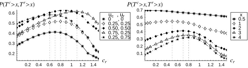
Problem 2 has also been solved for different choices of the total initial reserve u and the initial reserves of the cedent, uc and the reinsurer, ur. The impact of different initial
reserves on PHTc>x,Tr>xL and hence on the optimal value of cr is illustrated in the left
hcHtL=uc+H1.55-crLt, hrHtL=ur+crt, with u=uc+ur and c=cc+cr =H1.55-crL+cr. Five curves are given in the left panel of Fig 2 which
corre-spond to five different choices of the pair of values uc, ur, for which the total reserve u=uc+ur is correspondingly equal to 0.0, 1.0, 0.5, 1.0, 1.0. There are two effects
which can be observed. First, with the increase of the total reserve u, given uc=ur, (see
curves corresponding to Huc,urL=8H0, 0L,H0.25, 0.25L,H0.5, 0.5L<), the probability of
joint survival increases as can be expected. The second effect is that, for fixed value of the total reserve u=1, the optimal reinsurance premium cr is lower if uc<ur, increases
when uc=ur, and goes further up if uc>ur. Hence, the conclusion is that, if a direct
insurance company wants to pay less in reinsurance premium and at the same time wants to maximize its and the reinsurer's chances of survival, the company should seek for a reinsurer with initial reserves higher than its own reserves, which is a practically meaning-ful business strategy. In the alternative case, uc>ur, the optimal reinsurance premium is
much higher, since given the direct insurance company wants a maximum probability of joint survival, it has to pay much more in order to compensate the lower level of reserves kept by the reinsurer. But this clearly is not in favour of the direct insurer and is not what reinsurance is about.
In the right panel of Fig 2, we illustrate the impact of the time horizon x on the probabil-ity of joint survival and cr. As can be seen, PHTc>x,Tr >xL decreases for longer time
horizons, which is natural to expect. On the other hand, increasing x from 0.5 to 3 results in higher reinsurance premium, whereas further increase of x does not affect cr. This can
be explained with the higher possibility of arrival of large claims to the reinsurer as x initially goes up.
0.2 0.4 0.6 0.8 1 1.2 1.4 cr 0.2
0.3 0.4 0.5 0.6
PHTc>x,Tr>xL
0.25, 0.75 0.75, 0.25 0.50, 0.50 0.25, 0.25 0 , 0
uc , ur
0.2 0.4 0.6 0.8 1 1.2 1.4 cr 0.1
0.2 0.3 0.4 0.5 0.6 0.7
PHTc>x,Tr>xL
[image:13.595.75.476.488.598.2]4 3 2 1 0.5x
Fig. 2. Solutions to the optimality Problem 2: independent claim severities, ExpH1L distrib-uted, l =1, x=2, c=1.55, L= ¶, M =0.5; Left panel: u¥0, Right panel: u=uc=ur =0, x=0.5, 1, 2, 3, 4.
The solution of the optimization Problem 1 has been performed in the case of exponen-tially and Pareto distributed claim severities, both with unit mean, l =1, x=2 and hHtL=1.55 t. Thus, in Fig. 3 two 3D plots are given, which illustrate the behaviour of the probability of joint survival as a function of M and m=L-M when the premium income is equally shared, i.e. hcHtL=hrHtL for any t¥0. The left panel of Fig. 3 refers to
variance EHWL=VHWL=1, whereas the plot in the right panel is for Pareto claims with EHWL=1 and VHWL=3. As seen from both panels of Fig. 3, PHTc>x,Tr>xL has a single global maximum with respect to M and m. As with Problem 2, the existence of a unique solution of Problem 1 can be conjectured, but the proof is related with similar difficulties.
Solutions of Problem 1 for different choices of cr, i.e., for different proportions in which
the total premium income is shared, are summarized in Table 1. As can be seen, giving higher proportion of hHtL to the reinsurer causes the optimal retention level, M, to drop and the optimal limiting level, m, to increase. The latter is not surprising as the cedent's retained risk should decrease when the premium income, passed on to the reinsurer, increases.
Table 1. Optimal values of M and m, maximizing PHTc>x,Tr>xL in the case of
inde-pendent claim severities, ExpH1L distributed, with l =1, x=2,
hHtL=hcHtL+hrHtL=H1.55-crLt+crt.
maxM ,m PHTc>x, Tr>xL cr=0.25 cr=0.50 cr=0.775 cr=1.00 cr=1.25
M 0.4 0.3 0.3 0.2 0.001
m 0.1 0.3 0.7 1.2 >1.5
PHTc>x,Tr>xL 0.2 0.4 0.6 0.8 1 1.2 1.4
m=L-M 0.2
0.4 0.6 0.8 1 1.2 M 0.34 0.38 0.42 0.2 0.4 0.6 0.8 1 1.2
m=L-M
PHTc>x,Tr>xL
0.2 0.4 0.6 0.8 1 1.2 1.4
m=L-M 0.2
0.4 0.6 0.8 1 1.2 M 0.39 0.43 0.47 0.2 0.4 0.6 0.8 1 1.2
[image:15.595.66.496.88.263.2]m=L-M
Fig. 3. Solutions to the optimality Problem 1: independent claim severities, l =1, x=2, hHtL=hcHtL+hrHtL=H1.55-crLt+crt, cr=0.775. Left panel - exponentially distributed, EHWL=VHWL=1; Right panel - Pareto distributed, EHWL=1, VHWL=3.
1 2 3 4 w
0.2 0.4 0.6 0.8 1 1.2
fHwL Claim size distribution
Weibull,EHWL=1,VHWL=2.2 Pareto,EHWL=1,VHWL=3 Exp,EHWL=1,VHWL=1
0.2 0.4 0.6 0.8 1 1.2 1.4 m 0.3 0.35 0.4 0.45 0.5 0.55
PHTc>x,Tr>xL M=0.2
Weibull,EHWL=1,VHWL=2.2 Pareto,EHWL=1,VHWL=3 Exp,EHWL=1,VHWL=1
Fig. 4. Left panel - assumed probability density functions for the claim amounts Wi, i=1, 2, ...; Right panel - PHTc>x,Tr >xL as a function of the layer m, l =1, x=2, hHtL=hcHtL+hrHtL=H1.55-crLt+crt, cr=0.775.
The general conclusion based on these examples is that PHTc>x,Tr>xL is a relevant reinsurance risk optimization criterion, which complies with some basic principles driv-ing reinsurance risk assessment and pricdriv-ing decisions.
4.2 Dependent claim severities.
In what follows, we provide some very interesting results for the probability of joint non-ruin and the solutions of Problems 1 and 2, assuming dependence between the claim severities W1,W2, ... . We show how this dependence could be modelled, using copula
functions. The effect on PHTc>x,Tr>xL of the degree of dependence, modelled by the underlying copula parameter, and of the choice of the marginals, is also studied.
[image:15.595.92.485.349.476.2]will require highly multivariate copulas. The curse of dimensionality is overcome here due to the fast convergence of formula (4), for which only the first few terms in the sum-mation with respect to k are needed, in order to compute PHTc>x,Tr >xL with a reason-able accuracy. This allows us to use up to a five-variate copula in the numerical examples presented here.
Let H denote the k-dimensional distribution function of the random vector of consecu-tive claim amounts HW1, ..., WkL with continuous marginals F1, ..., Fk. Then, one can use
the well-known Sklar's theorem to represent H through a k-dimensional copula CHu1, ...,ukL, 0§uj§1, which depends on a set of parameters q, as HHw1, ...,wkL= CHF1Hw1L, ..., FkHwkLL. By changing the values of q within a specified
range, one can control the degree of dependence, in general, from extreme negative, through independence, to extreme positive dependence. To measure the dependence in the tails of the distributions of two consecutive claims W1 and W2, one can use the upper
and lower tail dependence coefficients, defined as
lL= limuØ0+CHu,uL êu
lU = limuØ1-H1-2u+CHu,uLL ê H1-uL
where lLœH0, 1D, lU œH0, 1D. The copula C has no upper (lower) tail dependence iff
lU =0 (lL=0). For example, in our context, lU >0 would mean that extremely large
insurance losses are likely to occur jointly. For further properties of copulas and related dependence measures we refer to Joe (1997). An extensive account on some actuarial applications of copulas can be found in Frees and Valdez (1998).
It should be noted that dependence between the components of the random vector
HW1, ...,WkL implies dependence between the components of the random vector HW1c, ..., WkcL and also between the components of HW1r, ...,WkrL, since Wi=Wic+Wir.
So, the two risk processes, Rtc and Rtr, which implicitly define PHTc>x,Tr>xL, also incorporate dependent claims, namely HW1c, ...,WkcL and HW1r, ...,WkrL. However, since formulae (4) and (14) involve the joint density function yHw1, ...,wkL of the random
vector HW1, ...,WkL, in order to compute PHTc>x,Tr>xL under dependence, we express
this density through the copula function as
(21) yHw1, ...,wkL=
∑kCHF
1Hw1L, ...,FkHwkLL
ÅÅÅÅÅÅÅÅÅÅÅÅÅÅÅÅÅÅÅÅÅÅÅÅÅÅÅÅÅÅÅÅÅÅÅÅÅÅÅÅÅÅÅÅÅÅÅÅÅÅÅÅÅÅÅÅÅÅÅÅÅÅÅÅÅÅÅÅÅÅ ∑w1... ∑wk
= ÅÅÅÅÅÅÅÅÅÅÅÅÅÅÅÅÅÅÅÅÅÅÅÅÅÅÅÅÅÅÅÅ∑kCHu1, ...,ÅÅÅÅÅÅÅÅÅÅÅÅÅukL
∑u1... ∑uk ‰i=1
k ∑
FiHwiL
ÅÅÅÅÅÅÅÅÅÅÅÅÅÅÅÅÅÅÅÅÅÅÅ ∑wi
=cHF1Hw1L, ...,FkHwkLL ‰ i=1
k
fWiHwiL
where cHu1, ..., ukL is the density of the copula C and fWiHwiL, i=1, ..., k are the
of these two choices on PHTc>x,Tr>xL and on the solutions of the optimality Problems 1 and 2. For the purpose, we have chosen C to be the k-dimensional Rotated Clayton copula, CRCl, and F1, ..., Fk to be identical WeibullHa, bL marginals.
Clayton and Rotated Clayton copulas are suitable for modelling dependence between claim severities. To see this, let us first introduce the Clayton copula, which is an Archimedean copula, with generator fHtL=t-q-1, q >0, defined as
CClHu1, ..., uk;qL=H⁄ik=1ui-q-k+1L -1êq
,
where 0§ui§1, i=1, ..., k and q œH0,¶L is a parameter. Its density is given by cClHu1, ..., uk;qL= qk ÅÅÅÅÅÅÅÅÅÅÅÅÅÅÅÅÅÅÅÅGHG1Hê1q+êqLkL H¤ik=1ui-q-1L H⁄ik=1ui-q-k+1L
-1êq-k
.
As q Ø0, the Clayton copula converges to the product copula with density cHu1, ...,ukL=1, which, as seen from (21), corresponds to independent claim amounts.
The degree of dependence increases as q increases. Further properties of the Clayton copula and its application in finance can be found in Cherubini et al. (2004).
In the general insurance context, it is of interest to consider the case in which the occur-rence of large claims is highly correlated with the emergence of further large claims. Hence, it is meaningful to use a copula with upper tail dependence. However, the Clayton copula has lower tail dependence with coefficient lL=2-1êq, which makes it convenient
for modeling dependence in the left tails of the marginal distributions, i.e. between very small claims. A typical example would be the joint occurrence of a large number of small motor insurance claims caused by a common (catastrophic) event, e.g. hail or bad driving conditions.
Based on the Clayton copula, one can model upper tail dependence using the multivariate Rotated Clayton copula, defined as
(22) CRClHu
1, ...,uk;qL=⁄ki=1ui-k+1+H⁄ik=1H1-uiL-q-k+1L -1êq
,
with density cRClHu1, ...,uk;qL=cClH1-u1, ..., 1-uk;qL and q œH0,¶L. The value
q =0 corresponds to independence as for CCl. A two dimensional version of (22) has been considered by Patton (2004). The Rotated Clayton copula has upper tail dependence with coefficient lU =2-1êq and is suitable for modeling dependence between extreme
insurance losses. The dependence structure, defined by a Rotated Clayton copula with parameter q =5, is illustrated in the left panel of Fig. 5 through a random sample of 500 simulated pairs Hu1,u2L. In the right panel, we give the corresponding simulated claim
amounts with joint distribution function HHw1,w2L=CRClHF1Hw1L,F2Hw2L;qL and
0 0.2 0.4 0.6 0.8 1
u1
0 0.2 0.4 0.6 0.8 1
u2
CRClHu1,u2;qL
0 1 2 3 4 5 6 7
w1
0 1 2 3 4 5 6 7
w2
[image:18.595.82.474.90.224.2]CRClHFHw1L,FHw2L;qL
Fig. 5. A random sample of 500 simulations from a bivariate Rotated Clayton copula, with dependence parameter q =5, marginals FªWeibullH1, 1LªExpH1L.
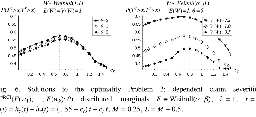
With the increase of q, the solution of the optimality Problem 2 does not change, as illustrated in the left panel of Fig. 6 for fixed Weibull marginals with unit mean and variance. It can also be seen that, for any cr, PHTc>x,Tr>xL goes up as q deviates from
zero. This may seem unexpected but it should be mentioned that, as q increases, not only the tail dependence increases but so does the dependence throughout the whole range of claim amounts. As a result of this, jointly small claims occur with higher probability and through the risk processes, Rtc and Rtr, affect more significantly PHTc>x,Tr>xL than the occurrence of jointly large claims.
0.2 0.4 0.6 0.8 1 1.2 1.4 cr 0.4
0.45 0.5 0.55 0.6 0.65 0.7
PHTc>x,Tr>xL
W~WeibullH1,1L EHWL=VHWL=1
q=0
q=1
q=5
0.2 0.4 0.6 0.8 1 1.2 1.4 cr 0.4
0.45 0.5 0.55 0.6 0.65 0.7
PHTc>x,Tr>xL
W~WeibullHa,bL EHWL=1,q =5
VHWL=0.5 VHWL=1.0 VHWL=2.2
Fig. 6. Solutions to the optimality Problem 2: dependent claim severities, CRClHFHw1L, ..., FHwkL;qL distributed, marginals F ªWeibullHa, bL, l =1, x=1, hHtL=hcHtL+hrHtL=H1.55-crLt+crt, M =0.25, L=M +0.5.
The solution of the optimality Problem 2 for Weibull marginals with mean 1 and increas-ing variance is given in the right panel of Fig. 6. As can be seen, the optimal value for cr
[image:18.595.78.505.433.629.2]increases which is a phenomenon, similar to the one illustrated in Fig. 4 and can be explained applying similar reasoning.
5. Conclusions and comments.
In this paper, we have demonstrated that the optimal retention and limiting levels and the optimal sharing of the premium income, obtained by maximizing the probability of joint survival of the cedent and the reinsurer in an excess of loss contract, assuming continuous claim severities, are sensible. It will be instructive to test this joint optimality criterion on real claim data.
An interesting finding is the presence of unique solutions to Problems 1 and 2 in the examples of Section 4.1. Proofs of such conjectures are a subject of ongoing research.
We have also demonstrated that formulae (4) and (14), through their reasonable general-ity, conveniently allow to implement copulas in modelling dependence between consecu-tive claim severities. These are only first steps in this important new direction of research and a variety of open problems arrises. For example, it is interesting to explore how the solutions of Problems 1 and 2, and also PHTc>x,Tr>xL, will be affected by different dependence structures. In particular, will the upper and lower Fréchet bounds lead to upper and lower bounds for PHTc>x, Tr >xL?
Finally, viewing PHTc>x,Tr>xL as a risk measure, one could define a performance measure based on the expected profits, at the end of the time horizon x, of the insurer and the reinsurer and consider an optimality criterion which combines these measures and could be used to optimally set the parameters of a reinsurance contract. The latter is a subject of future investigation.
References
Aase, K. (2002). Perspectives of Risk Sharing. Scand. Actuarial J., 2, 73-128.
Andersen, K.M. (2000). Optimal choice of reinsurance-parameters by minimizing the ruin probability. Thesis for the Degree Cand. Act., University of Copenhagen, Laboratory of Actuarial Mathematics.
Appell, P.E. (1880). Ann. Sci. École. Norm. Sup., 9, 119-144.
Bugmann, C. (1997). Proportional and non-proportional reinsurance. Swiss Re. Publications.
Centeno, M. L. (1997). Excess of loss reinsurance and the probability of ruin in finite horizon. ASTIN Bulletin, 27, 1, 59-70.
Cherubini, U., Luciano, E. and Vecchiato, W. (2004). Copula methods in finance. John Wiley and Sons Ltd.
Dickson, D.C.M. and Waters, H.R. (1996). Reinsurance and ruin. Insurance: Mathemat-ics and EconomMathemat-ics, 19, 1, 61-80.
Dickson, D.C.M. and Waters, H.R. (1997). Relative reinsurance retention levels. ASTIN Bulletin, 27, 2, 207-227.
Frees, E. and Valdez, E. (1998). Understanding Relationships Using Copulas. North American Actuarial Journal, v.2 No 1, 1-25.
Gerber, H. U. (1979). An Introduction to Mathematical Risk Theory. Monograph N 8, S.S. Huebner Foundation for Insurance Education, Wharton School, University of Pennsyl-vania, Philadelphia.
Hipp, C. and Vogt, M. (2001). Optimal dynamic XL reinsurance. Preprint No 1/01, Uni-versity of Karlsruhe.
Joe, H. (1997). Multivariate Models and Dependent Concepts. Chapman & Hall, London.
Ignatov, Z. G. and Kaishev, V. K. (2004). A finite time ruin probability formula for continuous claim severities. Journal of Applied Probability, 41, 570-578.
Ignatov, Z. G., Kaishev, V. K. and Krachunov, R. S. (2004). Optimal retention levels, given the joint survival of cedent and reinsurer. Scand. Actuarial J., 6, 401-430.
Kaishev, V. K. and Dimitrova, D. S. (2003). Finite time ruin probabilities for continuous claim severities. Actuarial Res. Paper 150, Cass Business School, City University, London.
Karlin, S. and Taylor, H. M. (1981). A Second Course in Stochastic Processes. Academic Press, New York.
Kaz'min Yu. A.(2002). Appell polynomials. Encyclopaedia of Mathematics, Edt. by Michiel Hazewinkel. Springer Verlag, Berlin.
Krvavych, Y. (2001). On existence of insurer's optimal excess of loss reinsurance strat-egy. Paper presented at the 5-th International Congress on Insurance:Mathematics and Economics.
Patton, A. (2004). On the Out-of-Sample Importance of Skewness and Asymmetric Depen-dence for Asset Allocation. Journal of Financial Econometrics, v.2, 130-168.
Schmidli, H. (2002). On minimizing the ruin probability by investment and reinsurance. Preprint, University of Aarhus.
Suijs, J., Borm, P. and De Waegenaere, A. (1998). Stochastic cooperative games in insur-ance. Insurance:Mathematics and Economics, 22, 209-228.
Taksar, M. and Markussen, C. (2003). Optimal Dynamic Reinsurance Policies for Large Insurance Portfolios. Finance and Stochastics, 7, 1, 97-121.