Numerical simulation of fully nonlinear interaction between steep waves and 2D floating bodies using the QALE-FEM method

      

City, University of London Institutional Repository

Citation

:

Yan, S. and Ma, Q. (2007). Numerical simulation of fully nonlinear interaction between steep waves and 2D floating bodies using the QALE-FEM method. Journal of Computational Physics, 221(2), pp. 666-692. doi: 10.1016/j.jcp.2006.06.046

This is the accepted version of the paper.

This version of the publication may differ from the final published

version.

Permanent repository link:

http://openaccess.city.ac.uk/4323/

Link to published version

:

http://dx.doi.org/10.1016/j.jcp.2006.06.046

Copyright and reuse:

City Research Online aims to make research

outputs of City, University of London available to a wider audience.

Copyright and Moral Rights remain with the author(s) and/or copyright

holders. URLs from City Research Online may be freely distributed and

linked to.

City Research Online: http://openaccess.city.ac.uk/ [email protected]

Editorial Manager(tm) for Journal of Computational Physics Manuscript Draft

Manuscript Number: JCOMP-D-05-00722R1

Title: Numerical simulation of fully nonlinear interaction between steep waves and 2D floating bodies using the QALE-FEM method

Article Type: Regular Article

Section/Category:

Keywords: QALE-FEM; Nonlinear water waves; Spring analogy method; Iterative procedure; 2D floating bodies

Corresponding Author: Dr Qingwei Ma, PhD

Corresponding Author's Institution: City University

First Author: Shiqiang Yan

Order of Authors: Shiqiang Yan; Qingwei Ma, PhD

Numerical simulation of fully nonlinear interaction between steep waves

and 2D floating bodies using the QALE-FEM method

S. Yan and Q.W. Ma

School of Engineering and Mathematical Sciences, City University, London, EC1V 0HB, UK

Abstract

This paper extends the QALE-FEM (Quasi Arbitrary Lagrangian-Eulerian Finite Element Method) based on a fully nonlinear potential theory, which was recently developed by the authors ([1], [2]), to deal with the fully nonlinear interaction between steep waves and 2D floating bodies. In the QALE-FEM method, complex unstructured mesh is generated only once at the beginning of calculation and is moved to conform to the motion of boundaries at other time steps, avoiding the necessity of high cost remeshing. In order to tackle challenges associated with floating bodies, several new numerical techniques are developed in this paper. These include the technique for moving mesh near and on body surfaces, the scheme for estimating the velocities and accelerations of bodies as well as the forces on them, the method for evaluating the fluid velocity on the surface of bodies and the technique for shortening the transient period. Using the developed techniques and methods, various cases associated with the nonlinear interaction between waves and floating bodies are numerically simulated. For some cases, the numerical results are compared with experimental data available in the public domain and good agreement is achieved.

Keywords: QALE-FEM; Nonlinear water waves; Spring analogy method; Iterative procedure; 2D floating bodies

1.

Introduction

With operations in the oil and gas industry moving to deeper water, offshore structures are more likely to be exposed to very harsh environments and extremely steep waves and therefore undergo large motions. As a result, there is an increasing interest in numerically simulating nonlinear water waves and their interaction with floating structures. Two classes of theoretical models for cases with finite water depth are in common use for numerical simulations. One is based on general flow theory and the other is based on potential theory. In the first class of models, the Navier-Stokes and continuity equations together with proper boundary conditions are solved; while in the second class, the Laplace equation with fully nonlinear boundary conditions are dealt with. For brevity, the first class of models will be called NS Model and the second called FNPT (representing fully nonlinear potential theory) Model in the paper.

solve the Navier-Stokes and continuity equations together with one of three formulations. However, whichever formulation is used, solving the NS equations is always a time consuming task. As a result, the FNPT Model has been employed in many publications for problems associated with nonlinear water waves and their interaction with structures. In this model, viscosity is ignored. The governing equations are dramatically simplified and therefore need much less computational resources to be solved than in the NS Model. Comparison with experimental data ([3]-[6]) has shown that the results obtained by using this model are accurate enough if breaking waves do not occur and/or if structures involved are large. Therefore, the FNPT Model, instead of the NS Model, should be preferred if a case considered falls in this category.

The problems formulated by FNPT model are usually solved by a time marching procedure suggested by Longuet-Higgins & Cokelet [7]. In this procedure, the key task is to solve the boundary value problem by using an efficient numerical method, such as the boundary element method (BEM) or the finite element method (FEM). The BEM has been attempted by many researchers, such as Vinje & Brevig [8] , Lin, Newman & Yue [9] , Wang, Yao & Tulin [10], Kashiwagi [11], Cao, Schultz & Beck [12], Celebi, Kim & Beck [13], Grilli, Guyenne & Dias [14] and Kim, Celebi & Kim [15]. The FEM has been developed by Wu & Eatock Taylor ([16],[17]) for two dimensional cases and by Ma, Wu & Eatock Taylor ([5],[6]) and Ma [18] for three dimensional cases. All the above publications are concerned with problems either about fixed bodies or those with a prescribed motion. Until now, the publications about the interaction between fully nonlinear waves and free-response bodies are still very limited. Beck & Schultz [19] made nonlinear computation of wave loads and motions of freely rectangular barge in incident waves. Tanizawa [20], Tanizawa & Minami [21] and Tanizawa, Minami & Naito [22] simulated 2D freely barge-type floating body, followed by Koo [23] and Koo & Kim [24]. Kashiwagi & Momoda [25] and Kashiwagi [26] investigated wave-induced motions of 2D complicated-shape floating body. All of them used the BEMs. Recently, Wu & Hu modelled the interaction between waves and a 3D cylindrical FPSO-like structure ([27]) in which the FEM was applied.

overcome the difficulty, Ma and Yan ([1] and [2]) have recently invented a QALE-FEM (Quasi Arbitrary Lagrangian-Eulerian Finite Element Method). The main idea of this method is that the complex unstructured mesh is generated only once at the beginning of calculation and is moved at other time steps to conform to motions of boundaries. This feature allows one to use an unstructured mesh with any degree of complexity without the need of regenerating it at every time step. Ma & Yan [1] compared the QALE-FEM with conventional FEM in terms of computational efficiency and accuracy in the cases with periodic bars on the seabed. They concluded that the QALE-FEM may require less than 15% of the CPU time required by the conventional FEM at the same accuracy level. However, they applied the new method only to cases without floating bodies.

In this paper, the QALE-FEM is extended to deal with problems involving 2D freely floating bodies. In order to tackle the challenges associated with floating bodies, several new numerical techniques are developed. These include a technique for moving the mesh near and on the body surface, a scheme for estimating the velocities and accelerations of bodies as well as the forces on them, a method for evaluating the fluid velocity on the surface of bodies and a technique for shortening the transient period. The last technique is beneficial to investigations of response amplitude operators (RAOs) of floating bodies in waves, which require reaching a steady state (all motions being periodic with roughly constant amplitudes) as soon as possible in order to save CPU time. Using these developed techniques, various cases associated with the nonlinear interaction between waves and floating bodies are numerically simulated. For some cases, the numerical results are compared with experimental data available in the public domain and good agreement is achieved.

2. Mathematical model and numerical method

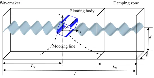
In this paper, waves are generated by a piston-like wavemaker in a tank as shown in Fig.1. The wavemaker is mounted at the left end and a damping zone with a Sommerfeld condition (see [5] and [18] for details) is applied at the right end of the tank in order to suppress the reflection. A Cartesian coordinate system is used with the oxy plane on the mean free surface and with the z-axis being positive upwards. A floating body is placed at x=0 initially and moored to the bed or walls of the tank.

2.1. FNPT model for fluid

Similar to the usual formulation for the FNPT Model, the velocity potential (

φ

) satisfies Laplace’s

equation,

0

2

₌

∇

φ

(1)

in fluid domain. On the free surfacez=

ζ

(

x,y,t

)

, the velocity potential satisfies the kinematic and dynamic conditions in the following Lagrangian form,

z

Dt

Dz

y

Dt

Dy

x

Dt

Dx

∂

∂

=

∂

∂

=

∂

∂

2

2

1

_φ

φ

∇

+

−

=

gz

Dt

D

(3)

where

Dt

D

is the substantial (or total time) derivative following fluid particles and g is the

gravitational acceleration. In Eq. (3), the atmospheric pressure has been taken as zero. On all rigid boundaries, such as the wavemaker and the floating body, the velocity potential satisfy

)

(

t

U

n

n

r

r

_⋅

=

∂

∂

φ

(4)

where and n are the velocity and the unit normal vector of the rigid boundaries, respectively. The positive direction of the normal vector points to the outside of the fluid domain.

( )

t

U

r

r

Wavemaker Damping zone

Floating body z

y

[image:6.595.178.443.295.429.2]

x

Fig. 1. Sketch of fluid domain

2.2. Motion equations of a floating body

The displacements, velocities and accelerations of a floating body are governed (see, e.g., [18] and [28]) by

F

U

M

]

r

&

_c

=

r

[

(5a)

N

I

I

]

Ω

r

&

+

Ω

r

×

[

]

Ω

r

=

r

[

(5b)

c

U

dt

S

d

r

r

=

(6a)

Ω

=

r

r

dt

d

B

]

θ

[

(6b)

where

F

r

and Nr are the force and moment acting on the floating body; Ur_cand

U

r

&

_c the translational

velocity and acceleration of its gravitational centre; Ω

r

and

Ω

r

&

its angular velocity and acceleration;

)

,

,

(

α

β

γ

θ

r

the Euler angles; S the translational displacements. In Eq. (5) and (6), [M] and [I] are mass and inertia matrixes, respectively; and [B] is the matrix formed by Euler angles and defined as,

r

L Mooring line

Lm

Lw

d

[ ]

⎥ ⎥ ⎥ ⎦ ⎤ ⎢ ⎢ ⎢ ⎣ ⎡ − = 1 0 sin 0 cos sin cos 0 sin cos cos

β

γ

γ

β

γ

γ

β

B (7)

In 2D cases,

Ω

r

×

[

I

]

Ω

r

=

0

,

α

=

0

,

γ

=

0

, Eqs (5b) and (6b) can be rewritten as

N

I

]

Ω

r

&

=

r

[

(8)

Ω

=

r

r

dt

d

θ

(9)

Once Ur_c and

Ω

r

are known, the velocity at a point on the body is determined by Ω

× + = r r r r

b c r

U

U (10)

where is the position vector relative to the gravitational centre.

r

_b

2.3. Force calculation

The force (

F

r

) and moment (Nr ) acting on a body in Eqs. (5) and (6) can be evaluated by,

m S f ds n gz t F b r r r ₊ ⎟ ⎠ ⎞ ⎜ ⎝ ⎛ _{+ ∇ +} ∂ ∂ −

=

∫∫

2

2

1

_φ

φ

ρ

(11)

m S

b nds N

r gz t N b r r r r + × ⎟ ⎠ ⎞ ⎜ ⎝ ⎛ _{+ ∇ +} ∂ ∂ −

=

∫∫

2

2

1

_φ

φ

ρ

(12)

where Sb denotes the wetted body surface. fm

r

and Nr_m are forces and moments due to mooring lines, respectively. Because this paper focuses on the wave-body interaction, the mooring lines are approximated by using linear springs, i.e.,

m m m k S

f r

r

= (13a)

m m m r f

Nr = r × r (13b)

in which km is the spring stiffness, Smis the displacement of the mooring point,

r

m

r

r

is the position

vector of the mooring point relative to the gravitational centre.

As can be seen, the time derivative of the velocity potential (

∂

φ

/

∂

t

) is required and is critical for

accurately calculating forces and moments. A simplest way to calculate

∂

φ

/

∂

t

is to use a backward

finite difference scheme:

t

t

n n n

∆

−

=

⎟

⎠

⎞

⎜

⎝

⎛

∂

∂

_φ

_φ

_φ

−1

(14)

find

∂

φ

/

∂

t

by solving a similar boundary value problem to that for

φ

defined in Eqs. (1)-(4) (see, for

example,[5]-[6], [16]-[18]). The boundary value problem for

∂

φ

/

∂

t

is defined by,

0

2

_⎟

₌

⎠

⎞

⎜

⎝

⎛

∂

∂

∇

t

φ

(15)

in the fluid domain. On the free surface z =

ζ

(

x,y,t

)

, it is given by

2

2

1

_φ

ζ

φ

₌

₋

₋

_∇

∂

∂

g

t

(16)

On all rigid boundaries, it satisfies

)]

(

[

]

[

φ

φ

φ

∇

−

×

∂

∂

⋅

Ω

+

∂

∂∇

⋅

−

⋅

×

Ω

+

=

⎟

⎠

⎞

⎜

⎝

⎛

∂

∂

∂

∂

c b c b

c

r

U

n

n

U

n

r

U

t

n

r

r

r

r

r

r

r

r

&

r

&

. (17)

It should be noted here that there is a difficult with solving Eqs. (15) to (17). As can be seen from

Eq. (17), the accelerations

U

r

&

_c and

Ω

r

&

should be known when solving the boundary value problem for

t

∂

∂

φ

/

. However, in cases involving a free-response floating body, they are evaluated by Eqs. (5) and (6), which depends on the force and moment given in Eqs. (11) and (12). In turn, to find the force and moment, one needs

∂

φ

/

∂

t

. The scheme to overcome this difficulty will be detailed in Section 5

below.

2.4. FEM formulation

The full details about the FEM formulation have been discussed in our previous publications, for example [1], [5] and [18]. They will not be repeated here. Only summary of the formulation is given below.

The problem described by Eqs. (1) to (4) will be solved by using a time step marching procedure. At each time step, the free surface and the potential values on it as well as velocities on all rigid boundaries are known. Thus, the boundary condition for the potential on the free surface can be replaced by a Dirichlet condition:

p

f

=

φ

(18)

where is the potential values on the free surface, which can be estimated by using Eq. (3) and a

time integration scheme with second order accuracy. Therefore, the unknown velocity potential in the fluid domain can be found by solving a mixed boundary value problem which is defined by Eqs. (1), (4) and (18). To do so, the fluid domain is discretised into a set of small tetrahedral elements and the

velocity potential is expressed in terms of a linear shape function,

p

f

(

)

N x y z

_J

, ,

:

∑

=

J J

J

N

(

x

,

y

,

z

)

φ

φ

(19)

boundary conditions are discretised as follows,

∑

∫∫∫

∫∫∫

∑

∫∫

∈ ∀ ∀ ∉ ∀ ∇ ⋅ ∇ − = ∀ ∇ ⋅ ∇ P n

P J S

J

J J p I

S I n S

J J

J J

I N d N f dS N f N d

N

φ

( ) (20)

where SP represents the Dirichlet boundary on which the velocity potential fp is known and Sn

represents the Numann boundary on which the normal derivative of the velocity potential fn is known.

Eq. (20) can further be written in the matrix form:

[ ]

A

{ } { }

φ

= B (21) where

{ }

φ

=

[

φ

₁,

φ

₂,

φ

₃,_K,

φ

_I,_K

]

T (I∉S_P) (22a)

(

_{P P}

J I

IJ N N d I S J S

A =

_∫∫∫

∇ ⋅∇ ∀ ∉ ∉ ∀

,

)

(22b)

(

P

)

S J J J p I S n I

I

N

f

dS

N

f

N

d

I

S

B

P n

∉

∀

∇

⋅

∇

−

=

_∫∫

_∫∫∫

∑

∀ ∈

)

(

(22c)

The algebraic Eq. (21) is solved by using a conjugate gradient iterative method with SSOR

pre-conditioner and optimised parameters [18]. The problem about

∂

φ

/

∂

t

described in Eqs. (15) to (17)

is also solved by using the above method with

φ

and the boundary conditions for it are replaced by

t

∂

∂

φ

/

and corresponding boundary conditions for

∂

φ

/

∂

t

.

3. Summary of

QALE-FEM

method

As indicated in the Introduction, the QALE-FEM developed in [1] will be extended in this paper to deal with problems with 2D floating bodies. In this section, the key elements of the QALE-FEM in [1] are summarised before presenting new developments of this paper.

3.1. Scheme for moving mesh

The main idea of the QALE-FEM is that the complex unstructured mesh is generated only once at the beginning of calculation and is moved at other time steps to conform to the motion of boundaries. Obviously, the technique for moving the mesh is crucial in this method to achieve high robustness and high efficiency. For this purpose, a novel methodology is suggested and adopted, in which interior nodes and boundary nodes are considered separately; the nodes on the free surface and on rigid boundaries are considered separately; nodes on the free surface are split into two groups: those on waterlines and those not on waterlines (inner-free-surface nodes); and different methods are employed for moving different nodes.

∑

∑

= =

∆

=

∆

i Ni

j ij N

j ij j

i

k

r

k

r

1 1

r

r

₍₂₃₎

where

∆

r

r

_i is the displacement at Node I; kijis the spring stiffness and Niis the number of nodes that

are connected to Node I. For problems about nonlinear water waves, it is crucial to maintain the quality (good element shapes and reasonable node distribution) of mesh near the free surface. To do so, the spring stiffness in the QALE-FEM is suggested as

( ) [ z z d]

ij

ij e i j

l

k = 1₂ γ1+ + 2 (24)

where kij is the spring stiffness, lij is the distance between Nodes I and J; zi and zj are the vertical

coordinates of Nodes I and J; d is the water depth; and γ is an coefficient that should be assigned a larger value if the springs are required to be stiffer at the free surface. The spring analogy method is also used for moving nodes on rigid boundaries.

The positions of nodes on the free surface are determined by physical boundary conditions, i.e., following the fluid particles at most time steps. The nodes moved in this way may become too close to or too far from each other. To prevent this from happening, these nodes are relocated at a certain frequency, e.g. every 40 time steps. When doing so, the nodes on the waterlines is re-distributed by adopting a principle for a self-adaptive mesh, i.e., the weighted arc-segment lengths satisfies

s i i

∆

s

=

C

ϖ

(25)

where ϖ is a weighted function,

∆

s

_i the arc-segment length between two successive nodes and Cs a

constant. In order to relocate the inner-free-surface nodes, they are first moved using the spring analogy system in the projected plane of the free surface, resulting in new coordinates x and y; and then the elevations of the free surface corresponding to the new coordinates are evaluated by an interpolating method. In order to take into account of the local gradient of the free surface, however, the spring stiffness for moving the nodes in x- and y- directions is determined, respectively, by:

( ) 2

2 1 1 ⎟ ⎠ ⎞ ⎜ ⎝ ⎛ ∂ ∂ + = x l k ij x ij ζ

and ( )

2 2 1 1 ⎟⎟ ⎠ ⎞ ⎜⎜ ⎝ ⎛ ∂ ∂ + = y l k ij y ij ζ . (26)

where ( )x and are the spring stiffness;

ij

k ( )y

ij k

x

∂

∂

ζ

and

y

∂

∂

ζ

the local slopes of the free surface in the x-

and y-directions, respectively. The numerical tests in [1] have shown that the scheme for moving mesh is very robust and very efficient.

3.2. Calculation of fluid velocities on the free surface

free surface is split into normal and tangential components. To estimate the normal component of the velocity, two points on the normal line at Node I are selected firstly and the velocity potentials at these

two points are then approximated by using a moving least square method. The normal component (

v

r

_n) of the velocity is determined by a three-point finite difference scheme:

n

h

h

h

h

h

h

h

h

h

h

h

v

_I I I I I I I I I I I I I I n

r

r

_⎥

⎦

⎤

⎢

⎣

⎡

⎟⎟

⎠

⎞

⎜⎜

⎝

⎛

+

+

⎟⎟

⎠

⎞

⎜⎜

⎝

⎛

+

−

⎟⎟

⎠

⎞

⎜⎜

⎝

⎛

+

+

+

=

₂ 2 1 1 2 1 1 2 2 1 2 1 1

3

2

1

3

2

2

1

2

3

2

_φ

_φ

_φ

. (27)

where I1 and I2 represent the two points selected; hI1 andhI2 are the distances between I and I1 and

between I1 and I2, respectively; and

φ

_I,

φ

_I1 and

φ

_I2 denote the velocity potentials at the node and the two points; the later two,

φ

_I1 and

φ

_I2, are found by a moving least square method. After the normal component of the velocity is determined, the tangential components of the velocity is calculated using a least square method based on the following equation

k k

k y k

x lIJ v lIJ lIJ vn lIJ

vr_τ ⋅r +r_τ ⋅r =r ⋅∇φ−r ⋅r ( k=1,2,3, ……, m) (28)

where

k

IJ

l

r

is the unit vector from Node I to Node Jk;

v

r

τ_x and vτy

r _{represent the velocity components}

in

τ

r

_x and

τ

r

_y directions, respectively. These directions are determined by

τ

r

_x

⊥

n

r

,

τ

r

_x

//

e

r

_x,

τ

r

_y

⊥

n

r

and

τ

r

_y

//

e

r

_y, where

e

r

_xand

e

r

_y are the unit vectors in the x- and y-directions, respectively.

4. Mesh moving scheme associated with floating bodies

The new developments of this paper for dealing with problems with a 2D floating body will be presented in the next three sections. They mainly contain three aspects: 1) mesh moving when a floating body is involved; 2) calculation of fluid velocities on the surface of the floating body and 3) estimation of velocities of the floating body and forces on it. The first aspect is presented in this section.

The basic strategy and principle to move the mesh are similar to that for the problem without floating bodies as summarised above. Nevertheless, special considerations must be devoted to the mesh near the body and on its surface, which is discussed in the following two subsections.

4.1. Moving interior nodes

( )

[1 2 ] (ˆ ˆ /2) 2

1 f zi zj d b wi wj

ij

ij _l e e

k = γ + + γ +

(29)

where

γ

_f is the same as

γ

in Eq. (24);

γ

_b plays the same role as

γ

_f but is used to adjust the spring stiffness near the body surface. The two coefficients may be different but in this paper they are taken

to be the same values, i.e.,

γ

_f

=

γ

_b

=

1

.

7

. In Eq. (29), is a weight function and is determined by, wˆ

⎩ ⎨ ⎧

≤ −

> =

f f f f

f f

D d D d

D d w

/ 1

0

ˆ (30a)

where df is the minimum distance from the node concerned to the body surface as shown in Fig. 2; Df

is the distance between the body surface and the boundary of the near-body-region and is defined as,

max

c f

d

D

=

ε

(30b)

where dcmax is the maximum distance from the gravitational centre to the wetted body surface and depends on the relative position of the floating body to the free surface. Numerical tests show that

ε

= 1.5 is suitable. It can be seen from Eq. (29) and (30) that the spring stiffness outside the near-body-region is the same as that for problem without a floating body.

[image:12.595.226.436.389.497.2]

Fig. 2 Region near floating body (GC: Gravitational centre)

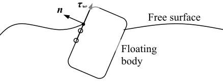
4.2. Moving nodes on body surfaces

The wetted body surface is time-dependent in the problems considered here. In order to conform to the change in the wetted body surface, the nodes on the surface must also be moved at each time step. The principle for doing so is similar to that for moving the nodes on the free surface, i.e., splitting the nodes into two groups: nodes on the waterline and nodes lying on the body surface but not on the waterline, the later called inner-body-surface nodes. For 2D problems, there are only two nodes on the waterline. They are moved by using the tangential velocity of the fluid relative to the body surface. The inner-body-surface nodes may appear to be moved by the same approach for moving inner-free-surface nodes, i.e., projecting the nodes onto a horizontal plane, moving the nodes in it by using the spring analogy method and then finding the new positions of nodes on the body surface by interpolation. This approach is obviously subjected to a condition that the surface must have only one

Free surface

GC

dcmax

Floating body

Df

I dmin

intersecting point with any vertical line; in other words, it can be expressed by a single-valued function. However, this is not always true for floating body surfaces, particularly when they undergo angular motions, such as roll and/or pitch. Therefore, one can not actually use the same approach as for moving the inner-body-surface nodes. A new approach is developed here. In this new approach, the spring analogy method is applied in a local coordinate system formed by the local tangential and normal lines. In this local coordinate system, the body surface is single–valued; i.e., there is only one intersecting point between the body surface and a line parallel to the local normal line (and, of course, perpendicular to the local tangential line). A node, e.g., i, is first moved along the tangential line by

∑

∑

= =

⋅

∆

=

∆

i Ni

j ij N

j

i ij

i

k

r

k

r

1 1

τ

τ

r

r

r

₍₃₁₎

where

τ

r

_i is the tangential direction at node i. After that, the new position of the nodes on the body surface is found by interpolation in the local coordinate system. The spring stiffness in Eq. (31) is

taken as k_ij =1/l_ij2.

It should be noted that at a sharp corner, there will be no unique tangential and normal lines and so the above approach fails. The remedy for overcoming the difficulty is to prescribe a node at the corner or to smooth the corner. Either way works well and gives similar results based on our numerical tests. It should also be noted that the new approach described in this sub-section may be employed to move inner-free-surface nodes when overturning waves are involved, though they are not considered in the paper.

5. Calculations of fluid velocity on the surface of the floating body

The velocity potential on the floating body surface always satisfies Eq. (4) and so the normal components of fluid velocity on the body surface can be determined by

) (

)

( _{c b}

n n U t n U r

vr = r⋅ r = v⋅ r +Ωv ×v (32)

[image:14.595.184.403.76.157.2]

Fig. 3 Definition of tangential and normal directions at a node on the waterline

6. Calculation of forces on and velocities of the floating body

In this paper,

∂

φ

/

∂

t

, involved in Eqs. (11) and (12) for estimating the forces on floating bodies,

is calculated by solving a boundary value problem defined in Eqs. (15)-(17). As discussed in Section 2.3, there is difficulty with doing so due to the nonlinear coupling between the body and wave motions. In order to tackle this difficulty, four types of methods have been suggested in the literature, i.e. the indirect method, the mode-decomposition method, the Dalen & Tanizawa’s method and the iterative method. The indirect method was developed by Wu & Eatock Taylor [16] and followed by Kashiwagi & Momoda [25] and Kashiwagi [26], Wu & Hu [27]. In this method, some auxiliary functions were introduced to decouple the mutual dependence between the force and the acceleration of the body. The mode-decomposition method was suggested by Vingi & Brevig [8] and adopted by Koo [23] and Koo & Kim [24]. In this approach, the body acceleration is decomposed into several modes (4 modes in 2D cases or 7 modes in 3D cases, respectively). Every mode is found by solving a boundary value problem similar to that for the velocity potential but under different boundary conditions. Using these modes and the body-motion equations, the body acceleration is determined. Both these methods have to solve 4 or 7 extra Laplace equations under different boundary conditions. The CPU time, therefore, may be considerably increased if employing an iterative procedure rather than a direct solution scheme (such as Gauss Elimination) which is unlikely to be suitable for solving the corresponding linear algebraic system containing a very large number of unknowns. In the method proposed by Dalen [30] and Tanizawa in [20] and [31], the body accelerations in Eq. (17) are implicitly substituted by the Bernoulli’s equations and thus the velocity potential and its time derivative are solved without the need of calculating accelerations of the floating bodies. However, this method requires one to form a

special matrix for

∂

φ

/

∂

t

which is different from the one for the velocity potential and whose

properties have not been sufficiently studied. This is likely to increase the difficulty for numerically

solving the algebraic equations associated with

∂

φ

/

∂

t

and also needs more CPU time for generating

the special matrix. That would be the main reason for this method not to be commonly used. Cao, Beck. & Schultz [19] suggested an iterative method to calculate the force and acceleration at each time step; in this way, the need to solve extra equations in the first two methods and the problem with the third method is eliminated.

For the purpose of time marching, a standard explicit 4th_{-order Runge-Kutta scheme is generally}

n

Free surface τw

used to update the velocity of the floating body, which requires three sub-step calculations at one time step forward. In each sub-step, the geometry of the computational domain may or may not be updated. If it is not updated, it is called a frozen coefficient method; if it is update, it is called a fully updated method. The CPU time spent on updating in the fully updated method is roughly equal to 4 times that in the frozen coefficient method. However, the frozen coefficient may not lead to stable and reasonable results for problems with large motions of floating bodies, as indicated by Koo & Kim [24]. The body velocity is estimated from the acceleration at previous time steps (or sub-steps) in all the above methods; i.e., the corresponding procedure is explicit. The explicit procedure may be satisfactory if time steps and so changes in the velocity and acceleration in one step are sufficiently small; otherwise, it may degrade the accuracy and even lead to instability.

In this paper, an improved iterative procedure, called Iterative Semi Implicit Time Integration Method for Floating Bodies (ISITIMFB), is developed, which takes some advantages and overcome some disadvantages of other methods. This method features by (a) using the acceleration in the current step to estimate the body velocity, i.e., it is implicit, distinguishing it from all other methods discussed above; (b) not requiring sub-step calculations, different from the fully updated Runge-Kutta method; (c) eliminating the necessity of solving the extra equations as in the indirect method and the mode-decomposition method and the need to generate a special matrix in the Dalen & Tanizawa’s method, getting rid of the main disadvantages of all three; (d) not updating the positions of the free surface and the floating body during the iteration to find the acceleration and force, saving the CPU time spent not only on this but also on forming the new coefficient matrix. The details of the method are described as follows.

Suppose that all calculations until t=tn-1 have been finished and so the velocity potential and its

time derivative on the free surface, the positions of all boundaries including the free surface and the body surface have been obtained through updating. To find the fluid and body velocities at time tn, the

following procedure is used.

1) Predict the body acceleration

A

r

n(0) at time tnby curve fitting of accelerations at previous

time steps using a least square method [34] and estimate the corresponding body velocity by using the Adams-Moulton method [35] as following,

( )

₍

₅

( )

₈

₎

12

2 1 0

1

0

₌

−

₊

₊

−

₋

n−

b n b n

b n

b n

b

A

A

A

t

U

U

r

r

∆

r

r

r

(33)

where

A

r

n(0) and represent the predicted values of translational or angular body accelerations and velocities, respectively, at the current time step, which are used as the initial values of iteration.

( )0

n b

Ur

surface.

4) Calculate the fluid velocity Vr_bn( )0 on the body surface.

5) Using the following loop to find the acceleration of and forces on the body:

(a) Solve the boundary value problem for

( )k n

t

⎟

⎠

⎞

⎜

⎝

⎛

∂

∂

φ

using

_A

r

n(k−1)_, n(k−1 _and

b

Ur ) n(k−1)

b

V

in its boundary condition on the body surface (Eq. (17)), where the subscript n(k-1) represent the variables at time tnbut at k-th iteration (k=1,2,3……);

(b) Calculate the forces or moments

F

r

n(k) and so the acceleration

[ ]

1

[

( )

(

)

( 1)

]

)

(k ₌ − n nk _{+ 1−} n n k−

n

b M F F

Ar α r α r ; (34)

in which mass matrix

[ ]

M should be changed to the moment matrix of the mass

[ ]

I ,

(Eq. (8)), if the annular acceleration and moment are concerned; (c) Estimate the new body velocity using the similar method to Eq. (33)

( )

(

5

( )

8

)

12

2 1

1 − −

−

₊

₊

₋

=

n b n b k n b n b k n

b

A

A

A

t

U

U

r

r

∆

r

r

r

; (35)

(d) Solve the boundary value problem for

φ

using Ur_bn( )k in Eq. (4) for the boundary condition on the body surface;

(e) Calculate the new fluid velocity Vr_bn( )k on the body surface;

(f) Check if the relative error of accelerations (or forces) is small enough; if not, go to a); otherwise go to 6).

6) Update the position of the body using the final body velocity and acceleration in the above loop by using the 3rd _{order Taylor expansion,}

dt

U

d

t

U

t

t

U

S

S

u n u n u n n b n b ) ( 3 ) ( 2 ) ( 1

6

2

r

&

r

&

r

r

r

+

₌

₊

_∆

₊

∆

₊

∆

(36)

where is the translational or annular displacement of the body to be used for the

calculation of the next time step; 1 + n b Sr ) (u n

Ur and

_U

r

_&

n(u) _{represent the final values of body} velocities and accelerations (translational or annular) in the above loop, respectively; and

dt

U

d

r

_&

n(u)

is calculated by using the finite difference scheme

(

U

U

)

t

dt

U

d

n(u)

₌

r

_&

n(u)

₋

r

_&

n−1(u)

_/

_∆

r

&

.

7) Calculate the fluid velocity on the free surface using the final velocity potential in the above loop.

8) Update the time derivative of the velocity potential on and the positions of the free surface using the same method as in [5] and [18].

As can be seen, an under-relaxation in Eq. (34) is employed in the iterative loop from (a) to (f) to improve the convergent efficiency. The value of αn _{is determined by}

) 0 ( 1 )

1 ( 1

) 0 ( 1 )

( 1

− −

− −

− −

= _n

b n

b

n b u n b n

A A

A A

α

(37)

where is the final value of the acceleration in the iteration at the previous step. This

expression is proposed by considering the fact that if one had known , the solution for

would have been found in one iteration through (a) to (f) and by assuming that . )

( 1u n b

A

−

1 −

n

α

) ( 1u n b

A

−

_α

n

_≈

_α

n−1

The efficiency of the iterative procedure is signified by the iterative counter (or the number of iterations) in the above loop - the smaller iterative counter the more efficient. One may understand that the iterative counter for a specified accuracy depends on the quality of the predicted velocity in Eq. (33) and three values of the acceleration in Eq. (35). The better prediction of the velocity and the closer values of the acceleration should lead to the smaller number of iterations. The quality of the predicted velocity and the values of the acceleration are in turn determined by the time step, the amplitude of the body motions and the natural frequency of the system. It is expected that the velocity is better predicted and three values of the acceleration becomes closer and hence the iterations is fewer if the time step and the amplitude are smaller and/or if the natural period is larger. For the given wave and the shape of the body, the largest motion amplitude is related to the natural period. Therefore, the two most important factors affecting the iterative counter may be the time step and the natural period. Their effects are to be investigated in Section 7.2.2.

This iterative procedure is distinguished from one in [19] by three aspects. (1): The velocity potential (and so the fluid velocity) is obtained in [19] by assuming that the body velocity in Eq. (4) is

estimated using the acceleration at the previous time step and thus the boundary value problem for

φ

is solved only once, i.e. without Step (d), in the above loop. Therefore the procedure in [19] is actually an explicit method as implied above. (2): The relaxation scheme in Eq. (34) and the corresponding relaxation coefficient in Eq. (37) are employed in this paper while it is not clear whether any relaxation is adopted in [19]. (3): The body velocity used in Eq. (4) is continually updated here by employing the scheme as given in Eqs. (33) and (35), while it needs to be evaluated only once in [19].

7. Validations and discussions

In this section, the QALE-FEM method is validated by comparing its numerical predictions with analytical solutions and published results from other papers. Unless mentioned otherwise, the parameters with a length scale are nondimensionalised by the water depth d; and other parameters, including the time and frequency, by

g d

t→τ / and ω→ω g/d .

7.1. Forced-motion bodies

Although the main aim of this paper is to simulate cases involving 2D free-response floating bodies, the case for a 2D body in forced motions is investigated in the first stage in order to validate the force calculation, in which the iteration loop discussed in the previous section becomes unnecessary since the body acceleration does not need to be found. The body in these cases is formed with a circular cylinder as the submerged part and vertical walls above it, as shown in Fig.4 (a). The

dimensionless radius of the cylinder (

R

_b)is 0.25. The initial mesh around the body is similar to that in Fig. 4(b) but much finer.

(a) floating body (b) initial mesh near the body Fig.4 Sketch of body motions and illustration of initial mesh

The displacement (

η

) of the body is specified by

)

sin(

)

(

τ

ω

τ

η

=

a

_{b b} (38)

where

a

_b and

ω

_b are the amplitude and circular frequency of the motion, respectively. The velocity

corresponding to Eq. (38) is . This implies that the floating body suddenly

gain a finite value of velocity from rest, which is not only practically impossible but also can result in

a numerical difficult ([32]-[33]). To avoid it, the velocity ) cos( )

(

τ

_b

ω

_b

ω

_b

τ

c a

Ur =

c

Ur is ramped as in [33] and given by

) 1 )( cos( )

(

τ

a

ω

ω

τ

eβτ

Ur_c = _{b b b} − (39a)

π

χω

β

=

−

_b

/

2

(39b)

where

χ

is a coefficient. The larger the value of

χ

, the shorter the time is, during which the effects of

free surface

Rb

the ramp function persist, though the value does not affect the final results. In this paper,

χ

=

5

is

used.

0 5 10 15 20 25

-0.004 -0.002 0.000 0.002 0.004 Fx τ ξ=0.526

0 5 10 15 20 25

-0.004 -0.002 0.000 0.002 0.004 Fz τ ξ=0.526

0 5 10 15 20

-0.004 -0.002 0.000 0.002 0.004 Fx τ ξ=0.750

0 5 10 15 20

-0.004 -0.002 0.000 0.002 0.004 Fz τ ξ=0.750

0 5 10 15

-0.004 -0.002 0.000 0.002 0.004 Fx τ ξ=1.000

0 5 10 15

-0.004 -0.002 0.000 0.002 0.004 Fz τ ξ=1.000

[image:19.595.91.492.126.342.2]

(a) forced sway (b) forced heave

Fig. 5 Comparison of force histories for cases for forced sway/heave with analytical solution (Solid line: numerical results, Dot line: analytical solution [36])

7.1.1. Comparison with the analytical solution

When the amplitude of the harmonic motion is small, the hydrodynamic force can be evaluated by summing the analytical added mass and radiation damping forces [36], which is used for comparison with numerical results to verify our method. For the numerical simulation, the total tank length is taken as L ≈ 30 with the length from the wavemaker to the body taken as Lw ≈ 15 (Fig. 1).

The motion amplitude in Eq. (38) are assigned as

a

_b

=

0

.

01

. The mesh is unstructured and there are about 35 elements on the free surface in each wave length. The time step is taken as T/128, where T

is the wave period. The x-direction hydrodynamic force (divided by ) in the forced sway and the

z-direction hydrodynamic force (also divided by ) in the forced heave are plotted in Fig.5 for

three cases with different values of

2

gd

ρ

2

gd

ρ

ξ

, where

_ξ

₌

_ω

_b2

R

_{b is the frequency parameter. It can be seen}

that the numerical results agree very well with the analytical ones in all the cases, except in the transient period when the difference is expected because the analytical forces are evaluated for steady state but not for the transient stage. To quantitatively show the accuracy of the numerical results, the relative error (Er) for the results in Fig. 5 is evaluated by:

a a n r f f f

where

=

∫

e

A

dA

f

f

2 _{; and are the numerical and analytical forces, respectively; and A}

n

f

f

_a e is the

duration over which the error is estimated. Because the accuracy of the forces within the transient period should not be of concern, Ae is taken as the total duration of simulation minus the transient

period (about half of wave period). The relative errors evaluated in this way for all the cases in Fig. 5 do not exceed 0.5%.

sway

-3 -2 -1

0.04 0.05 0.06 0.07 0.08 0.09 0.1 ds

log(

E

r)

T/40 T/64 T/128 T/200

heave

-3 -2 -1

0.04 0.05 0.06 0.07 0.08 0.09 0.1 ds

lo

g(

Er

)

T/40 T/64 T/128 T/200

[image:20.595.97.512.222.434.2]

(a) Sway (b) Heave

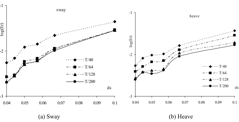
Fig. 6 The relative error for different meshes and different time steps

The characteristics of the relative error are further investigated by considering different time steps

and different mesh sizes. For this purpose, the relevant parameters are taken as

a

_b

=

0

.

01

and

ξ

=

0

.

75

(the corresponding wave length is about

λ

≈2.0), which are the same as the second case

relative errors are reduced with the decrease in mesh sizes and/or time steps, as expected. Particularly in the ranges of 0<ds<0.057 (about 35 elements in over one wave length) and , the relative errors are less than 0.8% for all these cases. This implies that the numerical results with a specified accuracy are achievable by using a sufficiently fine mesh and small time step.

64 / 0<dt<T

7.1.2. Forced motion with larger amplitudes

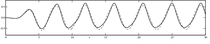
In order to investigate the nonlinear effects on waves generated by the forced-motions of the floating body, the cases similar to Fig. 5 but with larger amplitudes are simulated. The wave histories recorded on the left hand side of the body for the case with forced sway (ab=0.123) is depicted in Fig.7

together with that for ab=0.0041. Fig.8 shows the wave histories for the forced heave, in which the

solid line is the wave history for ab=0.082, while the dot line is that for ab=0.0041. In both figures, the

wave elevations are divided by the motion amplitude (ab).

0 5 10 15 20 25 30

-0.5 0.0 0.5

ζ/ab

[image:21.595.119.488.320.394.2]

τ

Fig.7 Wave history recorded at x=-1 due to forced sway (L=30, ωb=1.45,

ξ

=

0

.

75

, solid line: ab=0.123, dot line: ab=0.0041)

0 5 10 15 20 25 30

-0.5 0.0 0.5

ζ/ab

τ

Fig.8 Wave history recorded at x=-1 due to forced heave (L=30, ωb=1.45,

ξ

=

0

.

75

, solid line: ab=0.082, dot line: ab=0.0041)

[image:21.595.120.489.453.530.2]

-3 -2 -1 0 1 2 3 0.0

0.5 1.0 1.5

x

z

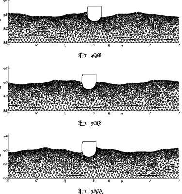
(a)τ≈14.50

-3 -2 -1 0 1 2 3

0.0 0.5 1.0 1.5

x

z

(b)τ≈15.80

-3 -2 -1 0 1 2 3

0.0 0.5 1.0 1.5

x

z

[image:22.595.113.488.81.479.2]

(c)τ≈16.66

Fig. 9 Mesh configurations for forced sway motion (L=30, ωb=1.45,

ξ

=

0

.

75

ab=0.123)

7.2. Free-response floating bodies

determined by

2

₂

tanh(

2

π

)

ω

π

λ

=

g

. In the following presentation, the frequency (ω) of the

wavemaker motion is represented by ; the force is nondimensionalised by using

on the assumption that the length of the 2D body in the direction parallel to the wavemaker is unit; and

the roll angle is nondimensionalised by , where is the amplitudes of incident waves.

Other parameters are nondimensionalised by the same way as in previous sections.

g B_b/2 2 ω

ξ =

_ρ

_gd

2

w w /g)A

(

ω

2

A

_w

7.2.1 Wavemaker ramp function and artificial damping technique

It is well known that the waves generated by a wavemaker in a tank are characterised by a transient wave profile in the front part of a wave train even though the motion of the wavemaker is purely harmonic. The transient wave profile often consists of several waves with different lengths and heights and a larger wave crest separating the transient and steady parts in the wave train. If one aims to investigate the properties of steady-sate responses, such as RAOs, of floating bodies, the transient waves and corresponding body responses are useless and hence they should be suppressed in order to reduce computational cost. Three methods may be used for this purpose. The first one is to apply wavemaker ramp functions that reduce the wave heights in the transient part. The second is to add artificial viscosity in the dynamic equations of floating bodies (called artificial damping technique), which diminishes the transient body responses. The third method is the combination of the first and the second ones. Details about them are given below.

Two wavemaker ramp functions are investigated, which are similar to those in [32] and [33]. The wavemaker motion corresponding to the first ramp function, called ‘Ramp1’, is governed by

( )

τ

a

cos

( )

ωτ

S

_w

=

−

, (41a)

),

sin(

)

(

τ

a

ω

ωτ

U

_w

=

(41b)

)

1

)(

cos(

)

(

_τ

_a

_ω

2

_ωτ

_e

βτ

U

&

_w

=

−

(41c)

where are the displacement, velocity and acceleration of the wavemaker respectively;

and the coefficient

w w

w

U

U

S

,

and

&

β

is the same as that in Eq.(39) with

ω

_b replaced by ω. In this approach, the

generated wave is not modified by the ramp function because the velocity of the wavemaker and so the velocity potential are not affected. The ramping is only performed on the acceleration of the

wavemaker, which implies that the value of ∂

φ

∂t and so forces on bodies are ramped. The wavemaker motion corresponding to the second ramp function, called ‘Ramp2’, is governed by

( )

τ

a

cos

( )

ωτ

r

(

τ

)

S

_w

=

−

, (42a)

τ

τ

)

=

∂

/

∂

(

_w

w

S

U

, (42b)

τ

τ

)

=

∂

/

∂

(

_w

w

U

[

]

⎩ ⎨ ⎧

≤ −

> =

f f

f

T T

T

r

τ

_πτ

τ

_τ

2 / ) / cos( 1 1 )

( (43)

where Tf is the cut-off time of the ramp function and is determined by

g w f L C

T =κ / (44)

in which κ is a coefficient between 0 and 1; and Cg is the group velocity of waves.

The efficiency of Ramp1 and Ramp 2 are investigated with

ξ

=

1

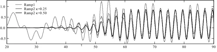
, a=0.0016, L ≈15 and Lw

≈10. The mesh used is unstructured with about 35 elements on the free surface in each wavelength. For the Ramp2, κ =0.25 and κ =0.5 are adopted for two cases, respectively.

20 30 40 50 60 70 80 90

-0.5 0.0 0.5 1.0

τ

[image:24.595.118.486.261.349.2]

sway motion/a Ramp1 Ramp2 κ=0.25 Ramp2 κ=0.50

Fig. 10 Sway motion by using different ramp functions

Fig. 10 shows the sway motions obtained by using different ramp functions. It can be observed that Ramp2 can make the calculation become steady sooner than Ramp1, though its effectiveness depends on the value of κ. It should be noted, however, that the waves at the wavemaker generated by

using Ramp2 during period τ <T_f are not the incident waves desired, implying that the waves at the floating body do not become the desired incident waves until τ >T_f +L_w/C_g. In addition, even after the desired incident waves arrive at the floating body, its responses exited by undesired waves do not

disappear immediately and so take extra time ( ) to become those excited by the desired waves. As a

result, the time history of motions during the time

e

T

e g w

f L C T

T + +

< /

τ should not be considered

when estimating RAOs. Based on this analysis, it is obvious that the shorter the sum of , the

less CPU time is required for estimating RAOs. As can be seen in Fig. 10, the transient period

becomes longer, indicating that T

e f T

T +

e becomes larger, with being shorter (i.e., smaller κ) when using

the Ramp2 only. Therefore, the reduction in does not necessarily lead to the reduction in the sum

of . The other option left to us is to reduce by using the artificial damping technique

mentioned above. With this technique, the motion equation, e.g., Eq. (5a), is modified to

f

T

f

T

e f T

T + T_e

F

U

U

M

]

&

_c

+

β

_{a c}

=

[

(45)

[

]

⎩ ⎨ ⎧

≤ +

> =

d d

c

d a

T T

T

τ

πτ

αβ

τ

τ

β

2 / ) / cos( 1 0 )

( (46)

where

β

_cis the critical damping corresponding to a motion component (such as sway or heave); α is a coefficient; and is the time during which the artificial damping is active. It is found by numerical

tests that and

d

T

g w d L C

T = / α =0.5 are appropriate for applications in this paper. Although this

technique may be used alone, we will only discuss numerical results obtained by combining it with the Ramp2 to shorten the length of the paper.

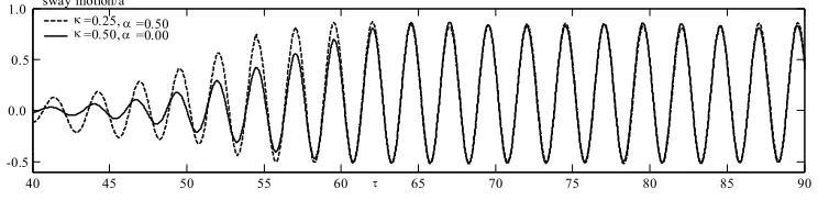
To show the effectiveness of the combined method, the two cases for the Ramp2 with κ =0.25 and κ =0.5in Fig.10 are considered again but in the first case, both the Ramp2 with κ=0.25 and the artificial damping technique with α =0.5 are applied. Fig. 11 gives the results, in which the dashed

line denotes the result from the combined method while the solid line represents the result obtained by only using the Ramp2 withκ=0.5. It is interesting to see that the response by the combined method

using 25κ =0. becomes steady at about

τ

=60, approximately two wave periods earlier than that by the Ramp2 alone with κ=0.5, which is steady at about τ =65. However, as shown in Fig. 10, the response corresponding toκ =0.25becomes steady much later than that to κ=0.5 when using the

Ramp2 alone. This indicates that the combined method is more effective to suppress the transient response.

40 45 50 55 60 65 70 75 80 85 90

-0.5 0.0 0.5 1.0

τ

sway motion/a

κ=0.25,α=0.50

[image:25.595.115.487.440.531.2]

κ=0.50,α=0.00

Fig. 11 Sway motion by using artificial damping technique

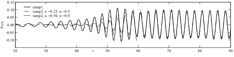
20 30 40 50 60 70 80 90 -0.10

-0.05 0.00 0.05 0.10 0.15

τ

Fx

/a

ramp1

[image:26.595.105.486.71.164.2]

ramp2, κ =0.25, α =0.5 ramp2, κ =0.50, α =0.0

Fig.12 Hydrodynamic force in cases with different ramp functions

7.2.2.The convergent properties of the ISITIMFB

One of developments in this paper is the suggestion of the ISITIMFB procedure to find the forces and the motions of the floating body. Its convergent properties, i.e. the iterative counter to achieve a specified accuracy, are presented and discussed in this subsection for the following case: the barge is similar to the one described at the beginning of Section 7.2; the length of the numerical tank is taken

as with ; and the dimensionless incident wave height generated is about 0.018 and the

frequency parameter is 13

≈

L

L

_w

≈

8

4

.

0

=

ξ

. Similar to above cases, the mesh used is unstructured with about 35 elements on the free surface in each wavelength. As has been discussed in Section 6, the two most important factors affecting the iterative counter are the time step and the natural period (frequency) of the system. Thus we mainly look at the convergent properties by changing the time step and the natural period in the following.

The results for different time steps are presented by three curves in Fig 13 (a), which correspond to three specified relative errors: 0.1%, 0.5% and 1%. In the figure, there are two rows of numbers under the horizontal axis. The first row represents the number of time steps in each wave period and the second row gives the length of the time step, i.e. the period divided by the number in the first row. In these cases, the mass of the floating body is the same as before, i.e. 125 kg. Under this condition,

the value of

ξ

based on the natural frequency is about 0.5 ~ 0.6 as shown by the experimental data in

[24]. One may observe from this figure that the iterative counter for a specified error decreases with the increase in the number of time steps in each period as expected. One may also observe that the convergence can be achieved within 10 iterations when the control error is 1% and the number of time steps in each period is larger than 64; and that reducing the control errors leads to the increase of iteration but not significantly. It should be noted that the wave frequency is near the natural frequency in these cases. For other cases (not presented) where the wave frequencies are much larger than the natural frequency, the convergent properties are better than those shown here.

The results corresponding to the different natural frequencies at three different control errors are depicted in Fig. 13b, which are obtained by artificially changing the mass in the range of

(m0: the mass for Fig. 13a) without changing the mooring stiffness and the

shapes of the floating body (i.e., the restoring coefficient being roughly fixed). Under this condition, the square of the natural frequency should be inversely proportional to the mass; and on this basis, the

0

0

100

1

.

iterative counter is plotted against the ratio of the mass to m0 rather than the frequency in the figure.

The time step is taken as T/128and all other parameters are the same as those in Fig.13(a). The results in Fig 13b indicate that the iterative counter varies with the change in mass or natural frequency but only in a small range for a large range of change in mass. Similar to Fig. 13a, the difference in the iterative counter does not change dramatically when the control error change from 0.1% to 1%. In addition, the iterative counter is smaller than 10 in the whole range of mass investigated for the control error of 1%.

Another point that needs to be discussed is how the control error in the ISITIMFB procedure affects the computed responses. Fig. 14 shows the comparison of roll motions obtained by using two different control errors for the cases of ∆t = T/64 in Fig. 13. It can be seen that the difference between the results is negligible. Therefore, one may consider the control error of 1% is acceptable in engineering practice but it is recommended that the computed results are compared with those by using a smaller control error such as 0.5%, which is followed when acquiring the numerical results in the paper.

4 5 6 7 8 9 10 11 12 13 14

40 80 120 160 200

time steps per wave period

It

er

ative

C

ounte

r

err=0.001 err=0.005 err=0.010

(0.06266) (0.031333) (0.020889) (0.015667) (0.012533) dt

(a) iterative counter vs time step

5 6 7 8 9 10 11 12 13 14

-1 0 1 2

log(m/m0)

It

er

ative

C

ounte

r

err=0.001 err=0.005 err=0.010

[image:27.595.202.418.360.491.2]

(b) iterative counter vs mass