Currency Premia and Global Imbalances

City, University of London Institutional Repository

Citation

:

10.1093/rfs/hhw038

This is the accepted version of the paper.

This version of the publication may differ from the final published

version.

Permanent repository link: http://openaccess.city.ac.uk/13287/

Link to published version

:

Copyright and reuse:

City Research Online aims to make research

outputs of City, University of London available to a wider audience.

Copyright and Moral Rights remain with the author(s) and/or copyright

holders. URLs from City Research Online may be freely distributed and

linked to.

Currency Premia and Global Imbalances

y

Pasquale DELLA CORTE

Steven J. RIDDIOUGH

Lucio SARNO

First submission: February 2014 - Revised: January 2016

Acknowledgements: We are grateful for comments and suggestions to Geert Bekaert (Editor), three anony-mous referees, Rui Albuquerque, Nicola Borri, Justinas Brazys, Craig Burnside, Alejandro Cuñat, Antonio Diez de los Rios, Carlo Favero, Xavier Gabaix, Federico Gavazzoni, Nicola Gennaioli, Leonid Kogan, Ralph Koijen, Matteo Maggiori, Lukas Menkho¤, Michael Moore, David Ng, Fulvio Ortu, Maik Schmeling, Astrid Schor-nick, Giulia Sestieri, Andreas Stathopoulos, Ilias Tsiakas and Adrien Verdelhan. We also thank participants at the 2015 CEPR Conference on “Macro-Financial Linkages and Current Account Imbalances”, 2015 ASSA meetings, 2015 Kiel Workshop on Exchange Rates, 2015 RCEA Money and Finance Workshop, 2013 WFA meeting, 2013 EFMA meeting, 2013 First Annual Conference on “Foreign Exchange Markets”, 2013 China In-ternational Conference in Finance, 2013 Asian Finance Association meeting, 2013 EFA conference, 2013 FMA meeting, 2013 Royal Economic Society Conference, Bank of Canada/Bank of Spain Workshop on “Interna-tional Financial Markets,” 2013 Interna“Interna-tional Paris Finance Meeting, 2012 Annual Conference on “Advances in the Analysis of Hedge Fund Strategies,” 2012 ECB-Bank of Italy Workshop on “Financial Determinants of Exchange Rates” and seminar participants at various institutions. We thank JP Morgan, Philip Lane, Gian Milesi-Ferretti and Jay Shambaugh for making data available which are used in this study. We gratefully acknowledge …nancial support from INQUIRE Europe. Steven Riddiough gratefully acknowledges …nancial support from the Economic and Social Research Council (ESRC), and Lucio Sarno acknowledges the gracious hospitality of the Cambridge Endowment for Research in Finance (CERF) of the University of Cambridge, where part of this research was conducted. The paper was the recipient of the Kepos Capital Award for the Best Paper on Investments at the 2013 WFA Annual Meeting. All errors remain ours.

y_{Pasquale Della Corte is with Imperial College Business School, Imperial College London and CEPR, email:}

Currency Premia and Global Imbalances

First version: February 2014 - Revised: January 2016

Abstract

We show that a global imbalance risk factor that captures the spread in countries’external

imbalances and their propensity to issue external liabilities in foreign currency explains the

cross-sectional variation in currency excess returns. The economic intuition is simple: net

debtor countries o¤er a currency risk premium to compensate investors willing to …nance

negative external imbalances because their currencies depreciate in bad times. This mechanism

is consistent with exchange rate theory based on capital ‡ows in imperfect …nancial markets. We also …nd that the global imbalance factor is priced in cross sections of other major asset

markets.

Keywords: Currency Risk Premium; Global Imbalances; Foreign Exchange Excess Returns;

Carry Trade.

1

Introduction

Imbalances in trade and capital ‡ows have been the centerpiece of much debate surrounding

the causes and consequences of the global …nancial crisis. Therefore it would seem natural

that, given the …nancial crisis consisted of collapsing asset prices worldwide, global imbalances may help shed light on our fundamental understanding of asset price dynamics. The foreign

exchange (FX) market provides a logical starting point for testing this hypothesis as exchange

rate ‡uctuations and currency risk premia are theoretically linked to external imbalances, and

recent events in the FX market provide a reminder of the potential importance of such a

link. For example, following the US Federal Reserve’s announcement on 22 May 2013 that it

would taper the size of their bond-buying programme, emerging market currencies including

the Indian rupee, Brazilian real, South African rand and Turkish lira all sold-o¤ sharply. A

common characteristic among these four countries is that they are some of the world’s largest debtor nations. In fact, the Financial Times on 26 June 2013 attributed the large depreciation

of the Indian rupee (which fell by 22% against the US dollar between May and August 2013)

to investors’concerns over India being “one of the most vulnerable emerging market currencies

due to its current account de…cit” (Ross, 2013).

In this paper we provide empirical evidence that exposure to countries’external imbalances

is key to understanding currency risk premia.1 _{Our …ndings are consistent with the broad}

im-plications of portfolio balance models, which emphasize the role of capital ‡ows for exchange

rate determination when assets denominated in di¤erent currencies are not perfectly substi-tutable. A recent notable example is the model of Gabaix and Maggiori (hereafter GM, 2015),

who provide a novel theory of exchange rate determination based on capital ‡ows in imperfect

…nancial markets. Speci…cally, GM (2015) propose a two-country model in which exchange

rates are jointly determined by global imbalances and …nanciers’risk-bearing capacity. In their

model, countries run trade imbalances and …nanciers absorb the resultant currency risk, i.e.,

1_{The results also support a risk-based interpretation of the carry trade, a popular strategy that borrows}

…nanciers are long the debtor country and short the creditor country. Financiers, however,

are …nancially constrained and this a¤ects their ability to take positions. Intuitively, if there

is little risk-bearing capacity …nanciers are unwilling to intermediate currency mismatches

re-gardless of the excess return on o¤er. In contrast, when …nanciers have unlimited risk-bearing

capacity they are willing to take positions in currencies whenever a positive excess return is

available, and hence the currency risk premium is miniscule. While this paper is not a direct test of the GM theory, our key results can be interpreted naturally under the description of

exchange rate determination o¤ered in this theory.

We focus the empirical analysis around two simple testable hypotheses, which we motivate

in Section 2. First, currency excess returns are higher when the funding (investment) country

is a net foreign creditor (debtor) and has a higher propensity to issue liabilities denominated

in domestic (foreign) currency. The relation between currency excess returns and net foreign

assets captures the link between external imbalances and currency risk premia in the theory

of GM (2015). The currency denomination of external debt also matters for currency risk premia. One argument why this may be the case, borrowed from the ‘original sin’literature

(e.g., Eichengreen and Hausmann, 2005), is that countries which cannot issue debt in their

own currency are riskier. In essence, this …rst testable hypothesis suggests that currency risk

premia are driven by the evolution and currency denomination of net foreign assets.

Second, we test the prediction of the GM (2015) theory that, when there is a …nancial

dis-ruption (i.e., risk-bearing capacity is very low and global risk aversion is very high), net-debtor

countries experience a currency depreciation, unlike net-creditor countries. This testable

hy-pothesis makes clear an important part of the mechanism that generates currency risk premia: investors demand a risk premium for holding net debtor countries’ currencies because these

currencies perform poorly in bad times, which are times of large shocks to global risk aversion.

After describing the data and portfolio construction methods in Section 3, we test and

provide empirical evidence in support of the two hypotheses described above. With respect

to the …rst testable hypothesis, we document in Section 4 that a currency strategy that sorts

currencies on net foreign asset positions and a country’s propensity to issue external liabilities

in domestic currency – termed the ‘global imbalance’ strategy – generates a large spread

in returns. Then, in Section 5 we empirically test whether a global imbalance risk factor

The global imbalance risk factor – termed the IM B factor, or simply IM B – is equivalent

to the return from a high-minus-low strategy that buys the currencies of debtor nations with

mainly foreign currency denominated external liabilities (the riskiest currencies) and sells the

currencies of creditor nations with mainly domestic currency denominated external liabilities

(the safest currencies). Our central result in this respect is thatIM B explains a large fraction

of the cross-sectional variation in currency excess returns, thus supporting a risk-based view of exchange rate determination that is based on macroeconomic fundamentals and, speci…cally,

on net foreign asset positions. This result holds both for a broad sample of 55 currencies and

for a subsample of 15 developed currencies over the period from 1983 to 2014.2

The economic intuition of this factor is simple: investors demand a risk premium to hold

the currency of net debtor countries, especially if the debt is funded principally in foreign

currency. For example, high interest rate currencies load positively on the global imbalance

factor, and thus deliver low returns in bad times when there is a spike in global risk aversion

and the process of international …nancial adjustment requires their depreciation. Low interest rate currencies are negatively related to the global imbalance factor, and thus provide a hedge

by yielding positive returns in bad times. This result suggests that returns to carry trades

are compensation for time-varying fundamental risk, and thus carry traders can be viewed as

taking on global imbalance risk. Importantly, the explanatory power of the global imbalance

risk factor is not con…ned to portfolios sorted on interest rate di¤erentials (i.e., carry trade

portfolios) and other interest rate sorts but extends to a broad cross section of currency

portfolios which includes, among others, portfolio sorts on currency value, momentum, and

volatility risk premia.

We also document how net foreign asset positions contain information that is (related but)

not identical to interest rate di¤erentials in the cross section of currencies. A regression of the

IM B factor on the carry (or ‘slope’) factor of Lustig, Roussanov and Verdelhan (2011)

pro-duces clear evidence that the two factors are signi…cantly di¤erent from each other, although

they are positively related. The main di¤erence between sorting on interest rate di¤erentials

(carry trade strategy) and sorting on global imbalances (global imbalance strategy) is in the

2_{There have hardly been any attempts to relate currency risk premiacross-sectionally to}

long portfolios of the two strategies: the riskiest countries in terms of net foreign asset

posi-tions are not necessarily the countries with the highest interest rates. Furthermore, our asset

pricing tests show that the global imbalance risk factor has pricing power in the cross-section

of currency excess returns even when conditioning on the carry risk factor. These …ndings

sup-port GM’s (2015) prediction that there is an e¤ect of net foreign asset positions on currency

excess returns that is distinct from a pure interest rate channel.3

In relation to the second testable hypothesis, in Section 6 we provide evidence using a

battery of panel regressions that in bad times (de…ned as times of risk aversion shocks, proxied

by the change in implied FX volatility) net-debtor countries experience a currency depreciation,

unlike net-creditor countries. This result is consistent with the risk premium story of GM

(2015): investors demand a risk premium for holding net debtor countries’currencies because

these currencies perform poorly in bad times.

Further analysis in Section 7 provides re…nements and robustness of the main results. For

example, in this analysis we test the pricing power of the IM B factor for cross-sections of returns in other markets, including equities, bonds and commodities. The results suggest that

theIM B factor is also priced in these asset markets. Overall, this additional analysis

corrob-orates the core …nding that global imbalance risk is a key fundamental driver of risk premia

in the FX market. Finally, we brie‡y summarize our key …ndings in Section 8. A separate

Internet Appendix provides further details on the data, robustness tests and additional results.

2

Theoretical Motivation and Testable Hypotheses

The contribution of this paper is purely empirical, but our analysis has a clear theoretical

foundation within the class of models centered around the portfolio balance theory. The

seminal work in the development of this theory is often attributed to Kouri (1976), who establishes a link between the balance of payments and exchange rates in a setting where assets

are imperfect substitutes, while risk averse investors are assumed to desire a diversi…ed portfolio

of risky securities. It follows that any deviation between the expected return on domestic and

foreign bonds leads to amarginal, rather than total, transfer of wealth between assets. The risk

3_{This result is also consistent with the empirical work of Habib and Stracca (2012), who …nd that net foreign}

aversion of investors, combined with the assumption that real sector adjustments are slower

than for the …nancial sector, mean that uncovered interest rate parity fails to hold within the

model. Instead, a domestic current account de…cit (capital account surplus) is associated with

a depreciation of the domestic currency.

Despite the early research breakthroughs relating to the portfolio balance model (e.g.,

Branson, Halttunen and Masson, 1979; Branson and Henderson, 1985), a combination of insu¢ cient data on foreign bond holdings, a lack of micro-foundation in deriving the

asset-demand functions and an early body of evidence documenting a weak relationship between

the balance of payments and exchange rate returns has led to a steady and prolonged decline

in the research agenda. Recently GM (2015) provide a modern micro-founded version of the

portfolio balance model by incorporating an interaction between capital ‡ows and …nancial

intermediaries’risk-bearing capacity in imperfect …nancial markets.

A distinct feature of the GM model is that global imbalances are a key driver of currency

risk premia: net debtor currencies are predicted to warrant an excess currency return in equilibrium and to depreciate at times when risk-bearing capacity falls. In their two-period

model –termed the ‘Gamma’model –each country borrows or lends in its own currency and

global …nancial intermediaries absorb the exchange rate risk arising from imbalanced capital

‡ows. Since …nancial intermediaries demand compensation for holding currency risk in the

form of an expected currency appreciation, exchange rates are jointly determined by global

capital ‡ows and by the intermediaries’ risk-bearing capacity, which GM (2015) refer to as

‘broadly de…ned risk aversion shocks’and show that it depends on conditional FX volatility.

GM (2015, equation (23), Proposition 6) derive the expected currency excess return as follows:

E(RX) =

R

RE(imp1) imp0

(R + )imp0+R_RE(imp1)

(1)

whereE( )is the expectation operator, andRX is the dollar excess return. The variableimpt

denotes the dollar value of US imports at timet; with exports normalized to unity in equation

(1), E(imp1) imp0 determines the evolution of net exports. In the basic Gamma model with

two periods and two countries, this setting implies a positive relation between the evolution

of net exports and net foreign assets since the external account must balance at the end of

risk-bearing capacity of …nanciers. When risk-risk-bearing capacity is low (i.e., is high), …nancial

intermediaries are unwilling to absorb any imbalances, regardless of the expected excess return

available, and hence no …nancial ‡ows are necessary as trade in‡ows and out‡ows will be equal

in each period. As risk-bearing capacity increases ( decreases), expected excess returns fall

but do not entirely disappear, except when is extremely low and …nancial intermediaries

are prepared to absorb any currency imbalance so that uncovered interest rate parity holds. Equation (1) shows that expected excess returns will be higher when interest rate di¤erentials

are larger (carry trade), and when the funding (investment) currency is issued by a net creditor

(debtor) country. Put another way, currency investors require a premium to hold the currency

of debtor nations relative to creditor nations.4

The Gamma model makes the simplifying assumption that each country borrows or lends

in its own currency, but in practice most countries do not (or cannot) issue all their debt in

their own currency. This fact is studied in the vast literature on the ‘original sin’hypothesis

(e.g., Eichengreen and Hausmann, 2005, and the references therein). Although GM (2015) do not provide a full analytical extension of their model that allows for currency mismatches

between assets and liabilities, in Proposition 12 (point 3) they consider the impact of

pre-existing stocks of debt and their currency denomination, illustrating how this generates a

valuation channel to the external adjustment of countries whereby the exchange rate moves

in a way that facilitates the re-equilibration of external imbalances. GM (2015) highlight how

this mechanism is consistent with the valuation channel to external adjustment studied by

Gourinchas and Rey (2007), Gourinchas (2008), and Lane and Shambaugh (2010), and gives

a role to the currency denomination of external liabilities. We note, however, that short of a full analytical description of the causal structure of foreign currency denominated debt, which

is not provided by GM (2015), one cannot dismiss possible endogeneity concerns as to why

countries issue debt in foreign currencies. Riskier countries may be forced to issue a higher

proportion of foreign currency denominated debt due to, for example, political instability or

4_{To clarify these e¤ects analytically in equation (1), …rst consider the case whenR =R >1, i.e., the interest}

rate in the foreign (investment) country is higher than the one in the funding country (the US). GM show that _@@E_(R(RX_R)₎ >0, which means that the expected currency excess return increases with higher interest rate di¤erentials. Second, set E[imp1] imp0>0 (while settingR =R= 1), i.e., the funding country (the US) is a net foreign creditor. Given that impis the value of US imports in US dollars,E[imp1] imp0 >0implies that the US is expected to become a net importer att= 1in order to o¤set its positive external imbalance at t= 0, and clearly _@(E(@E_imp(RX)

1) imp0) >0. This establishes the result that the expected excess return is higher if

in‡ation-induced expropriation risks. With these caveats in mind, in our empirical analysis we

account for the impact of foreign currency denominated debt by considering whether currencies

of countries with a higher propensity to issue liabilities in foreign currency o¤er a higher

currency risk premium, given that such countries require much sharper depreciations to correct

their external imbalances.5

The mechanism described above implies the …rst testable hypothesis, which is a variant of Proposition 6 in GM (2015) with the additional condition that captures the e¤ect of the

currency denomination of liabilities.

Hypothesis 1The expected currency excess return is bigger when (i) the interest rate

dif-ferential is larger, (ii) the funding (investment) country is a net foreign creditor (debtor), and

(iii) the funding (investment) country has a higher propensity to issue liabilities denominated

in domestic (foreign) currency.

This testable prediction suggests that, in addition to interest rate di¤erentials (condition

(i)) which have been analyzed extensively in the literature, FX excess returns are driven by the evolution of external debt and its currency denomination (conditions (ii) and (iii)). In

our portfolio analysis, we focus on this aspect of Hypothesis 1 and combine the information in

conditions (ii) and (iii) to capture both the spread in external imbalances and the propensity

to issue external liabilities in foreign currency. We also examine their separate e¤ects in some

of our tests and in the regression analysis.

We test Hypothesis 1 in several ways. Above all, we form portfolios sorted on external

imbalances (net foreign assets to GDP ratio) and the share of foreign liabilities in domestic

currency to examine whether they provide predictive information for the cross-section of cur-rency excess returns. We show that this portfolio sort generates a sizable and statistically

signi…cant spread in returns: a currency strategy that buys the extreme net debtor countries

with the highest propensity to issue external liabilities in foreign currency and sells the extreme

creditor countries with the lowest propensity to issue liabilities in foreign currency –which we

term the ‘global imbalance’strategy –generates Sharpe ratios of 0.59 for a universe of major

countries and 0.68 for a broader set of 55 countries. This con…rms the essence of Hypothesis

1, that currency excess returns are higher for net-debtor countries with higher propensity to

5_{This is because the initial depreciation makes countries with foreign-currency denominated liabilities}

issue liabilities in foreign currency. We also show that the returns from the global imbalance

strategy are related to but di¤erent from carry trade returns, consistent with the notion that

external imbalances partly capture di¤erent information from interest rate di¤erentials.

A central mechanism in the model of GM (2015) is that during periods of …nancial distress,

when risk-bearing capacity declines, debtor countries su¤er a currency depreciation, unlike

creditor countries. This is indeed the logic that rationalizes why net debtor countries must o¤er a currency risk premium, implying the second empirical prediction we take to the data,

which is Proposition 2 of GM (2015).

Hypothesis 2 When there is a …nancial disruption ( increases), countries that are net

external debtors experience a currency depreciation, while the opposite is true for net-creditor

countries.

This prediction follows naturally from the previous analysis and our empirical results

pro-vide supporting epro-vidence on its validity through the estimation of a battery of panel regressions.

Some caveats are in order on the theoretical motivation for our empirical work. First, in the empirical analysis we use implied volatility indices for FX (VXY) and equity markets

(VIX) to capture global risk aversion, but do not provide direct evidence that these proxies

are in fact driven by the wealth of …nancial intermediaries. GM (2015) state that conditional

volatility drives risk-bearing capacity, but we do not have a direct measure for this concept,

and VXY and VIX may well be capturing many other things. Second, within the GM (2015)

model, interest rates are modelled statically, as the inverse of the investor time preferences. An

extended model could incorporate global imbalances as one of the …nancial drivers of interest

rates and by doing so generate a positive albeit imperfect correlation between imbalances and interest rates. Third, as mentioned earlier, for tractability reasons GM (2015) assume that

countries can borrow and lend only in their own currencies and hence a full analytical treatment

of the decision to issue debt in foreign currency is not provided. However, our empirical work

does not make this assumption and we use the share of external liabilities issued in foreign

currency to re…ne our empirical characterization of the riskiness of global imbalances. Fourth,

it may be that our empirical …ndings can be rationalized by other theories, even in a complete

markets setting. In fact, Colacito, Croce, Gavazzoni and Ready (2015) have recently developed

a frictionless risk-sharing model of the international economy with recursive preferences and

of the carry factor of Lustig, Roussanov and Verdelhan (2011) and the global imbalance risk

factor proposed in our paper.

To be clear, therefore, it is not our purpose to discriminate between alternative theories

capable of rationalizing our …ndings or to provide a test of the theory of GM (2015); we

simply use that theory as a modern example of the portfolio balance approach to exchange rate

determination, in order to construct testable and economically plausible empirical hypotheses. This paper then aims at providing a robust empirical assessment of these hypotheses in order

to show novel facts about the link between global imbalances and currency risk premia.

3

Data and Currency Portfolios

This section describes the main data employed in the empirical analysis. We also describe the

construction of currency portfolios and the global imbalance risk factor.

Data on Currency Excess Returns. We collect daily spot and 1-month forward

exchange rates vis-à-vis the US dollar (USD) from Barclays and Reuters via Datastream.

Exchange rates are de…ned as units of US dollars per unit of foreign currency so that an increase in the exchange rate indicates an appreciation of the foreign currency. The analysis

uses monthly data obtained by sampling end-of-month rates from October 1983 to June 2014.

The sample comprises 55 countries, and we call this sample ‘all countries’. Since many

currencies in this broad sample are pegged or subject to capital restrictions at various points

in time, we also consider a subset of 15 countries which we refer to as ‘developed countries’.

The list of countries is in the Internet Appendix, which also provides further details about the

FX data.

We de…ne spot and forward exchange rates at timetasStandFt, respectively, and take into account the standard value date conventions in matching the forward rate with the appropriate

spot rate (see Bekaert and Hodrick, 1993). The excess return on buying a foreign currency in

the forward market at time t and then selling it in the spot market at time t+ 1 is computed

as

RXt+1 =

(St+1 Ft) St

which is equivalent to the spot exchange rate return minus the forward premium

RXt+1 =

St+1 St St

Ft St St

: (3)

According to the CIP condition, the forward premium approximately equals the interest rate di¤erential. Since CIP holds closely in the data (e.g., Akram, Rime, and Sarno, 2008), the

currency excess return is approximately equal to the exchange rate return plus the di¤erential

of the foreign interest rate and the US interest rate. As a matter of convenience, throughout

this paper we refer to f dt= (St Ft)=St as the forward discount or interest rate di¤erential

relative to the US. We construct currency excess returns adjusted for transaction costs using

bid-ask quotes on spot and forward rates. We describe in the Internet Appendix the exact

calculation of the net returns.

Data on External Assets and Liabilities. Turning to macroeconomic data, we obtain end-of-year series on foreign assets and liabilities, and gross domestic product (GDP) from

Lane and Milesi-Ferretti (2004, 2007), kindly updated by Gian Maria Milesi-Ferretti. Foreign

(or external) assets are measured as the dollar value of assets a country owns abroad, while

foreign (or external) liabilities refer to the dollar value of domestic assets owned by foreigners.

The data for all countries included in our study are until the end of 2012. For each country

we measure external imbalances –the indebtedness of a country to foreigners –using the net

foreign asset position (the di¤erence between foreign assets and foreign liabilities) relative to

the size of the economy (GDP), which we denote nf a. We retrieve monthly observations by keeping end-of-period data constant until a new observation becomes available.

We also use end-of-year series on the proportion of external liabilities denominated in

domestic currency (denoted ldc) from Benetrix, Lane and Shambaugh (2015), which updates

the data from Lane and Shambaugh (2010), kindly provided by Philip Lane. Clearly, measuring

accurately the share of external liabilities in foreign currency is a very hard task, also because

of the well-known di¢ culties in gathering data on derivatives positions. These data are, to

the best of our knowledge, the only ones available for this purpose that cover a large sample

of countries over a long span of time, from 1990 to 2012. We construct monthly observations by keeping end-of-period data constant until a new observation becomes available. Note that

we maintain the 1990 proportions back until 1983.6

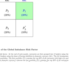
Global Imbalance Portfolios. Motivated by the considerations discussed in Section 2,

we construct global imbalance portfolios as follows: at the end of each period t, we …rst group

currencies into two baskets using our key sorting variable, i.e. nf a, then reorder currencies

within each basket using ldc. Hence, we allocate this set of currencies to …ve portfolios

so that Portfolio 1 corresponds to creditor countries whose external liabilities are primarily

denominated in domestic currency (safest currencies), whereas Portfolio 5 comprises debtor countries whose external liabilities are primarily denominated in foreign currency (riskiest

currencies). We refer to these portfolios as the global imbalance portfolios. As for all other

currency portfolios we consider, we compute the excess return for each portfolio as an equally

weighted average of the currency excess returns within that portfolio and, for the purpose of

computing portfolio returns net of transaction costs, we assume that investors go short foreign

currencies in Portfolio 1 and long foreign currencies in the remaining portfolios. We construct

the global imbalance (IM B) risk factor as the di¤erence between Portfolio 5 and Portfolio 1.

Figure 1 clari…es the outcome of our sequential sorting procedure. Note that the procedure does not guarantee monotonicity in both sorting variables (nf a and ldc) because Portfolio

3 contains both low and high ldc countries. However, the corner portfolios contain the

in-tended set of countries: speci…cally, Portfolio 1 contains the extreme 20% of all currencies

with high nf a and highldc (creditor nations with external liabilities mainly in domestic

cur-rency) whereas Portfolio 5 contains the top 20% of all currencies with low nf a and low ldc

(debtor nations with external liabilities mainly in foreign currency). We use …ve portfolios

rather than six, as we have a limited number of currencies in the developed countries sample

and at the beginning of the all countries sample, while we also want to have the same number of portfolios for both samples of countries. In the Internet Appendix we show that our core

results are qualitatively identical if we use 4 portfolios for developed countries and 6 portfolios

for all countries; see Figure A.1 and Table A.14 in the Internet Appendix.

Carry Trade Portfolios. We construct …ve carry trade portfolios, rebalanced monthly,

following the recent literature in this area (e.g., Lustig, Roussanov and Verdelhan, 2011). We

use them as test assets in our empirical asset pricing analysis, alongside a number of other

currency portfolios. At the end of each periodt, we allocate currencies to …ve portfolios on the

basis of their forward discounts. This exercise implies that currencies with the lowest forward

discounts (or lowest interest rate di¤erential relative to the US) are assigned to Portfolio 1,

whereas currencies with the highest forward discounts (or highest interest rate di¤erential

relative to the US) are assigned to Portfolio 5. The strategy that is long Portfolio 5 and short

Portfolio 1 is referred to as the CAR factor, or simply CAR.

Momentum Portfolios. Following Menkho¤, Sarno, Schmeling, and Schrimpf (2012b), at the end of each month t we form …ve portfolios based on exchange rate returns over the

previous k months. We assign the 20% of all currencies with the lowest lagged exchange

rate returns to Portfolio 1 (loser currencies), and the 20% of all currencies with the highest

lagged exchange rate returns to Portfolio 5 (winner currencies). We construct …ve short-term

momentum (k = 3 months) and …ve long-term momentum (k = 12 months) portfolios.

Value Portfolios. At the end of each period t, we form …ve portfolios based on the lagged 5-year real exchange rate return as in Asness, Moskowitz and Pedersen (2013). We

assign the 20% of all currencies with the highest lagged real exchange rate return to Portfolio

1 (overvalued currencies), and the 20% of all currencies with the lowest lagged real exchange

rate return to Portfolio 5 (undervalued currencies).

Term Spread and Long Yields Portfolios. We also construct …ve currency portfolios

sorted on the term spread of interest rates, and …ve currency portfolios sorted on the long-term interest rate di¤erential relative to the US, thus using additional information about interest

rates. We collect 3-month interest rates as proxy for short-term rates, and 10-year interest rates

(or 5-year when 10-year is not available) to capture the long-term rates from Global Financial

Data. Sorting on the term spread is motivated by the evidence in Ang and Chen (2010), while

sorting on long-term interest rates is useful to capture departures from uncovered interest rate

parity at the longer end of the term structure of interest rates (e.g., Bekaert, Wei and Xing,

2007). At the end of each month t, similar to the previous strategies, we sort currencies into

…ve portfolios using either the term spread or the long-term interest rate di¤erential. We assign the 20% of all currencies with the lowest term spread (lowest long-term interest rate

di¤erential) to Portfolio 1, and the20%of all currencies with the highest term spread (highest

long-term interest rate di¤erential) to Portfolio 5. This gives us …ve portfolios sorted on the

Risk Reversal Portfolios. At the end of each month t, we form …ve currency portfolios

using the 1-year implied volatility of currency option risk-reversals. For this exercise, we

update the implied volatility of currency options quoted over-the-counter used by Della Corte,

Ramadorai and Sarno (2015), who study the properties of this strategy in order to capture a

skewness risk premium in FX markets. For each currency in each time period, we construct

the 25-delta risk reversal, which is the implied volatility of an option strategy that buys a

25-delta out-of-the-money call and sells a25-delta out-of-the-money put with 1-year maturity.

We then construct …ve portfolios and assign the 20% of all currencies with the highest risk

reversal to Portfolio 1 (low-skewness currencies), and the20%of all currencies with the lowest

risk reversal to Portfolio 5 (high-skewness currencies). Finally, we compute the excess return

for each portfolio as an equally weighted average of the currency excess returns (based on spot

and forward exchange rates) within that portfolio.

Volatility Risk Premium Portfolios. At the end of each periodt, we group currencies

into …ve portfolios using their 1-year volatility risk premium as described in Della Corte, Ra-madorai and Sarno (2015). The volatility risk premium is de…ned as the di¤erence between the

physical and the risk-neutral expectations of future realized volatility. Following Bollerslev,

Tauchen, and Zhou (2009), we proxy the physical expectation of future realized volatility at

time t by simply using the lagged 1-year realized volatility based on daily log returns. This

approach requires no modeling assumptions and is consistent with the stylized fact that

re-alized volatility is a highly persistent process. The risk-neutral expectation of the future

realized volatility at time t is constructed using the model-free approach of Britten-Jones and

Neuberger (2000) which employs the implied volatility of 1-year currency options across …ve di¤erent deltas, i.e., 10-delta call and put, 25-delta call and put, and at-the-money options.

The volatility risk premium re‡ects the costs of insuring against currency volatility

‡uctua-tions and is generally negative. We construct …ve portfolios and allocate20%of all currencies

with the lowest volatility risk premia to Portfolio 1 (expensive volatility insurance currencies),

and 20%of all currencies with the highest volatility risk premia to Portfolio 5 (cheap volatility

insurance currencies). We then compute the excess return for each portfolio as an equally

weighted average of the currency excess returns (based on spot and forward exchange rates)

We have described above 9 currency strategies for a total of 45 portfolios. These strategies

are rebalanced monthly and the sample runs from October 1983 to June 2014. The sample

for the risk reversal and volatility risk premium portfolios, however, starts in January 1996

due to options data availability. These portfolios, for both sample periods analyzed, display a

correlation ranging from just over 30% to over 90%, with the average being around 70%. This

broad set of portfolios goes well beyond carry or interest rate-sorted portfolios, and will form our test assets in the asset pricing analysis.

4

The Global Imbalance Strategy and the Carry Trade

4.1

Portfolio Returns and the

IM B

Factor

This section describes the properties of the currency excess returns from implementing the

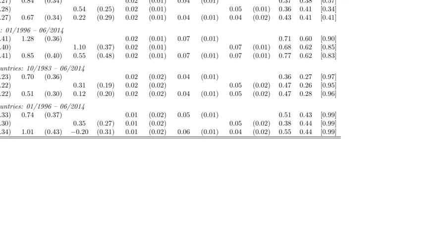
global imbalance strategy and constructing the IM B factor. In Table 1 we present summary

statistics for the …ve global imbalance portfolios sorted onnf aandldc, as well as for the global

imbalance factor IM B. The average excess return tends to increase from the …rst portfolio

(0:92% and 0:67% per annum) to the last portfolio (5:32% and 4:65% per annum) for both

samples. When we compare the Sharpe ratio (SR) of the global imbalance strategy to theSR

of the carry trade strategy (see Table A.1 in the Internet Appendix), we observe that the global

imbalance strategy has a Sharpe ratio that is at least as high as the carry trade strategy: 0.68 compared to 0.65 for all countries, and 0.59 compared to 0.43 for developed countries. This

comparison suggests that the global imbalance strategy has appealing risk-adjusted returns in

its own right, which is perhaps surprising given the information required to update the global

imbalance strategy arrives only once a year.7

The last three rows in Table 1 report the average f d, nf a, and ldc across all portfolios.

The spread in interest rate di¤erentials is about 7% and 3.5% for all countries and developed

countries, which is a large spread but far less than the 11% and 6% reported for the carry

trade in Table A.1. This suggests that part of the return from the global imbalance strategy is clearly related to carry (interest rate information), but part of it is driven by a di¤erent

7_{Speci…cally, we construct monthly excess returns but global imbalance portfolios are in practice rebalanced}

source of predictability which is in external imbalances but not in interest rate di¤erentials.

The last two rows reveal that there is a sizable spread in nf a andldc, which is monotonic for

nf a in both samples of countries examined and is much larger than the corresponding spread

for carry trade portfolios.

Overall, the currencies of net debtor countries with a relatively higher propensity to issue

external liabilities in foreign currency have higher (risk-adjusted) returns than the currencies of net creditor countries with higher propensity to issue liabilities in domestic currency, consistent

with Hypothesis 1 stated in Section 2.

4.2

IMB versus CAR

Since sorting on nf a and ldc delivers a set of portfolios with increasing interest rate

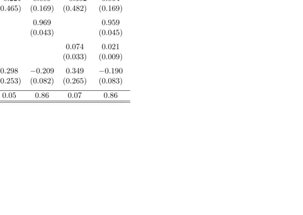
di¤er-entials, one may wonder whether IM B captures anything more than CAR. To investigate

this we …rst regress theIM B factor on the CARfactor and a constant term; in an additional

regression, we also control for the 12-month lag of the dependent variable to account for

po-tential serial correlation in theIM B factor (recall that the raw information aboutnf aandldc

is updated at the annual frequency). The results, reported in Panel A of Table 2, indicate that

the slope coe¢ cient ( ) estimate on CAR is positive and statistically signi…cant, but is far

and statistically di¤erent from unity (approximately 0.40). The R2 of the contemporaneous regression of IM B on CAR is 30%. Most importantly, the constant term ( ) is statistically

di¤erent from zero in all speci…cations and economically sizable (up to 2.3% per annum),

sug-gesting that IM B and CAR are di¤erent from each other. Indeed, the null hypothesis that

= 0 and = 1 (i.e., the null that IM B =CAR) is strongly rejected.

To further re…ne our understanding of the di¤erences between these two portfolio sorts, we

then run regressions of the …ve global imbalance portfolios on theCAR factor and a constant

term, again allowing for a 12-month lag of the dependent variable in separate regressions. The

results, reported in Panel B of Table 2, suggest that there is a moderate spread in the coe¢ cient

on theCARfactor, which is often statistically signi…cant. The in the regression is generally statistically insigni…cant, except in Portfolios 4 and 5 for the sample of all countries and in

Portfolio 5 for the sample of developed countries. Hence the di¤erence between the global

imbalance strategy and the carry trade strategy arises mainly from the long leg of the strategies

increasing interest rates, the countries with the worst global imbalance positions (in terms of

net foreign assets and the currency denomination of foreign debt) are not necessarily the

countries with the highest interest rates. This is also apparent when examining the identity

of the currencies that enter the long leg of the two strategies (see Table A.2 in the Internet

Appendix), which reveals, for example, that currencies like the Danish krone or the Swedish

krona are among the top six in Portfolio 5 of the global imbalance strategy due to their weak net foreign asset positions over much of the sample. Typical carry currencies like the Brazilian

real or the South African rand do not even feature among the top six most frequent currencies

in the long leg of the global imbalance strategy.

Taken together, the results reported till now suggest that the global imbalance strategy

has creditable excess returns overall, and that these returns are positively but imperfectly

correlated with the returns from the carry trade. The lack of a perfect correlation is in line

with Hypothesis 1 and the predictions of GM (2015), which states that global imbalances

matter for the determination of currency risk premia regardless of the size of interest rate di¤erentials. We now turn to a more rigorous investigation of the importance of global

imbalance risk using formal asset pricing tests applied to a broad set of currency portfolios.

5

Does Global Imbalance Risk Price Currency Excess

Returns?

This section presents cross-sectional asset pricing tests for currency portfolios and the global imbalance risk factor, and empirically documents that global imbalance risk is priced in a

broad cross-section of currency portfolios. Also, we …nd that the IM B factor is priced even

when controlling for the CAR factor of Lustig, Roussanov and Verdelhan (2011).

Methodology. We denote the discrete excess returns on portfolio j in period t as RX_tj.

In the absence of arbitrage opportunities, risk-adjusted excess returns have a price of zero and

satisfy the following Euler equation:

Et[Mt+1RX

j

t+1] = 0 (4)

with a Stochastic Discount Factor (SDF) linear in the pricing factors ft+1, given by

where b is the vector of factor loadings, and denotes the factor means. This speci…cation

implies a beta pricing model where the expected excess return on portfolio j is equal to the

factor risk price times the risk quantities j. The beta pricing model is de…ned as

E[RXj] = 0 j (6)

where the market price of risk = fb can be obtained via the factor loadings b. f =

E (ft ) (ft )0 is the variance-covariance matrix of the risk factors, and j are the re-gression coe¢ cients of each portfolio’s excess return RX_tj₊₁ on the risk factorsft+1.

The factor loadings b entering equation (4) are estimated via the Generalized Method of

Moments (GM M) of Hansen (1982). To implement GM M, we use the pricing errors as a

set of moments and a prespeci…ed weighting matrix. Since the objective is to test whether

the model can explain the cross-section of expected currency excess returns, we only rely on

unconditional moments and do not employ instruments other than a constant and a vector of

ones. The …rst-stage GMM estimation used here employs an identity weighting matrix, which

tells us how much attention to pay to each moment condition. With an identity matrix,

GM M attempts to price all currency portfolios equally well. The tables report estimates of b and , and standard errors based on Newey and West (1987) with optimal lag length

selection set according to Andrews (1991). The model’s performance is then evaluated using

the cross-sectionalR2 _{and theHJ distance measure of Hansen and Jagannathan (1997), which}

quanti…es the mean-squared distance between the SDF of a proposed model and the set of

admissible SDFs. To test whether the HJ distance is statistically signi…cant, we simulate p

-values using a weighted sum of 21-distributed random variables (see Jagannathan and Wang,

1996; Ren and Shimotsu, 2009).

The estimation of equation (6) is also undertaken using a two-pass ordinary least squares

regression following Fama and MacBeth (1973), and a two-step GMM estimation. Our results,

however, are virtually identical and therefore we only present one-step GMM estimates below.8

Risk Factors and Pricing Kernel. The most recent literature on cross-sectional asset

pricing in currency markets has considered a two-factor SDF. The …rst risk factor is the

8_{We also calculate the} 2 _{test statistic for the null hypothesis that all cross-sectional pricing errors (i.e.,}

expected market excess return, approximated by the average excess return on a portfolio

strategy that is long in all foreign currencies with equal weights and short in the domestic

currency – the DOL factor. For the second risk factor, the literature has employed several

return-based factors such as the slope factor (essentially CAR) of Lustig, Roussanov, and

Verdelhan (2011) or the global volatility factor of Menkho¤, Sarno, Schmeling and Schrimpf

(2012a). Following this literature, we consider a two-factor SDF with DOL and IM B as risk factors to assess the validity of the theoretical prediction in Hypothesis 1 that currencies more

exposed to global imbalance risk o¤er a higher risk premium. We also employ the two-factor

SDF with DOL and CAR as in Lustig, Roussanov and Verdelhan (2011), and a three-factor

SDF with DOL, CAR and IM B. The latter, three-factor SDF allows us to assess whether

IM B has any independent pricing power beyondCAR or simply mimicks information already

embedded in CAR. Moreover, in the Internet Appendix (Table A.17) we show that using the

global equity market excess return rather than DOL as the …rst factor does not a¤ect our

results.

Cross-Sectional Regressions. Table 3 presents the cross-sectional asset pricing results. The test assets include the following 35 currency portfolios for the sample from October

1983 to June 2014: 5 carry trade, 5 global imbalance, 5 short-term momentum and 5

long-term momentum, 5 value, 5 long-term spread, and 5 long yields portfolios. For the sample from

January 1996 to June 2014, we augment the above set of test assets with 5 risk reversal and 5

volatility risk premium portfolios, yielding a total of 45 currency portfolios. Lewellen, Nagel

and Shanken (2010) show that a strong factor structure in test asset returns can give rise to

misleading results in empirical work. If the risk factor has a small (but non-zero) correlation with the ‘true’ factor, the cross-sectional R2 _{could still be high suggesting an impressive}

model …t. This is particularly problematic in small cross sections, and it is a key reason why

we employ such a broad set of currency portfolios rather than just focusing, for example, on

the 5 carry portfolios.

Since IM B is a tradable risk factor, its price of risk must equal its expected return, i.e.

the price of global imbalance risk cannot be a free parameter in estimation. When the test

assets include the global imbalance portfolios, this problem does not arise. However, when

conducted later in the paper on cross-sections of equity, bond and commodity portfolios) we

follow the suggestion of Lewellen, Nagel and Shanken (2010) and include the global imbalance

factor as one of the test assets. This e¤ectively means that we constrain the price of risk for

IM B to be equal to the mean return of the traded global imbalance portfolio. The same logic

applies to CAR.

The results from implementing asset pricing tests on the above cross sections of currency portfolios as test assets are presented in Table 3, which reports estimates of factor loadings

b, the market prices of risk , the cross-sectional R2_{, and the HJ distance. Newey and West}

(1987) corrected standard errors with lag length determined according to Andrews (1991) are

reported in parentheses. The p-values of the HJ distance measure is reported in brackets.

The results are reported for all three SDF speci…cations described above, both for all countries

and for developed countries, and over two sample periods.

Starting from Panel A of Table 3, we focus our interest on the sign and the statistical

signi…cance of IM B, the market price of risk attached to the global imbalance risk factor. We …nd a positive and signi…cant estimate of IM B, in the range between 4% and 8% per annum

for all countries, and between 3% and 6% per annum for developed countries. The estimates

are very similar for both SDF speci…cations involving theIM B factor, i.e. also when the SDF

includes CAR. A positive estimate of the factor price of global imbalance risk implies higher

risk premia for currency portfolios whose returns comove positively with the global imbalance

factor, and lower risk premia for currency portfolios exhibiting a negative covariance with

the global imbalance factor. The standard errors of the risk prices are approximately equal

to 1% for all estimations carried out. The price of risk associated with IM B is more than two standard deviations from zero, and thus highly statistically signi…cant in each case. We

observe satisfactory cross-sectional …t in terms of R2_{, which ranges from 49% to 65% for the}

two-factor SDF that includesDOLandIM B. Further support in favor of the pricing power of

IM B comes from the fact that theHJ distance is insigni…cant. It is also worth noting that the

SDF speci…cation with DOL and CAR (hence not including IM B), does well in pricing the

test assets, as CARis statistically signi…cant, theR2is satisfactory (albeit lower than the SDF speci…cations involving IM B), and the HJ distance is not signi…cant. However, the bottom

line for our purposes is that a simple two-factor model that includes IM B performs well in

or notCARis included as a risk factor in the model. In turn, the latter point corroborates the

results in the previous section, suggesting that there is some di¤erential information embedded

in IM B versus CAR.

Panel B of Table 3 reports the same information as Panel A for asset pricing tests conducted

on test assets that now exclude both carry trade and global imbalance portfolios; hence the

number of test assets is 25 from 1983, and 35 from 1996. This exercise is an interesting out-of-sample test since we attempt to price currency portfolios that do not include the portfolios

from which IM B and CAR are constructed (although we do include the IM B and CAR

factors as test assets to ensure arbitrage-free estimates of IM B and CAR). The estimation

results reported in Panel B are qualitatively identical to the results in Panel A, indicating that

the pricing power of IM B recorded earlier is not driven simply by its ability to price global

imbalance and carry portfolios, but it clearly extends to other currency portfolios.9

Note that we do not argue that these two determinants of currency risk premia (global

imbalances and interest rate di¤erentials) are unrelated, only that they are imperfectly corre-lated. It is well-documented that there is a cross-sectional correlation between interest rates

(typically real interest rates) and net foreign asset positions (e.g., Rose, 2010). In Table 4,

we present results from a cross-sectional regression of the nominal interest rate di¤erentials

used in our study on net foreign assets and the share of liabilities denominated in domestic

currency. These results show clearly that net foreign assets enter the regression with a strongly

statistically signi…cant coe¢ cient and with the expected sign: higher nf a is associated with

lower interest rates. The R2 is lower than one might expect, however, suggesting that there may be important omitted variables in the regression. Indeed, when we add in‡ation di¤eren-tials and output gap di¤erendi¤eren-tials to the regression, net foreign asset positions remain strongly

signi…cant, but the R2 _{increases dramatically, mainly due to in‡ation di¤erentials.}10 _{In short,}

the main point is that, even though the information in global imbalances is related to

inter-est rate di¤erentials, there is independent information in global imbalances that matters for

currency returns.

9_{We also replace the dollar factor with the global equity factor (W EQ) which we proxy using the returns}

on the MSCI World Index minus the 1-month US interest rate but asset pricing results remain qualitatevely similar. We collect the data from Datastream and report the results in the Table A.17 in the Internet Appendix.

10_{In‡ation and the output gap are the core variables in macro models of the short-term interest rate,}

Portfolios based on IM B Betas. We provide evidence of the explanatory power of

the IM B factor for currency excess returns from a di¤erent viewpoint. We form portfolios

based on an individual currency’s exposure to global imbalance risk, and investigate whether

these portfolios have similar return distributions to the global imbalance portfolios. If global

imbalance risk is a priced factor, then currencies sorted according to their exposure to global

imbalance risk should yield a cross section of portfolios with a signi…cant spread in average currency returns.

We regress individual currency excess returns at time t on a constant and the global

imbalance risk factor using a 36-month rolling window that ends in period t 1, and denote

this slope coe¢ cient as i_{IM B;t}. This exercise provides currencyiexposure toIM B only using

information available at time t. We then rank currencies according to i_{IM B;t} and allocate

them to …ve portfolios at time t. Portfolio 1 contains the currencies with the largest negative

exposure to the global imbalance factor (lowest betas), while Portfolio 5 contains the most

positively exposed currencies (highest betas). Table 5 summarizes the descriptive statistics for these portfolios. We …nd that buying currencies with a low beta (i.e., insurance against

global imbalance risk) yields a signi…cantly lower return than buying currencies with a high

beta (i.e., high exposure to global imbalance risk). The spread between the last portfolio and

the …rst portfolio is in excess of 5% per annum for both sets of countries. Average excess

returns generally increase, albeit not always monotonically, when moving from the …rst to

the last portfolio. Moreover, we also …nd a clear monotonic increase in both average

pre-formation andpost-formation betas when moving from Portfolio 1 to Portfolio 5: they line up

well with the cross-section of average excess returns in Table 1. Average pre-formation betas vary from 0:22 to 1:35 for all countries, and from 0:94 to 0:67 for developed countries.

Post-formation betas are calculated by regressing the realized excess returns of beta-sorted

portfolios on a constant and the global imbalance risk factor. These …gures range from 0:06

to0:69for all countries, and from 0:29to0:82for developed countries. Overall, these results

con…rm that global imbalance risk is important for understanding the cross-section of currency

6

Exchange Rates and Net Foreign Assets in Bad Times

We now turn to testing Hypothesis 2, as stated in Section 2. In essence, the testable prediction

from GM (2015) that we take to the data is that exchange rates are jointly determined by

global imbalances and …nanciers’risk-bearing capacity so that net external debtors experience a currency depreciation in bad times, which are times of large shocks to risk bearing capacity

and risk aversion ( is high in the model). In contrast, net external creditors experience a

currency appreciation in bad times.

In the model of GM (2015), is driven by shocks to conditional FX volatility. We use the

change in the VXY index as a proxy for conditional FX volatility risk to proxy , i.e. shocks

to the willingness of …nanciers to absorb exchange rate risk. VXY is the FX analogue of the

VIX index, and is a tradable volatility index designed by JP Morgan. It measures aggregate

volatility in currencies through a simple, turnover-weighted index of G7 volatility based on 3-month at-the-money forward options. In general, GM (2015) refer to as loosely proxying

for global risk aversion shocks, and therefore we also show in the Internet Appendix (Tables

A.6, A.7 and A.9) the robustness of our results using the change in VIX, a commonly used

proxy for global risk aversion in the empirical …nance literature.11

We test Hypothesis 2 in two di¤erent ways. First, we estimate a panel regression where we

regress monthly exchange rate returns on a set of macro variables, allowing for …xed e¤ects. As

right-hand-side variables, we employnf alagged by 12 months, and the interest rate di¤erential

lagged by 1 month. In some speci…cations we also include ldc, and the change in VXY on its own. Importantly, we also allow for an interaction term between nf a as well as the interest

rate di¤erential and the change in the VXY index (speci…cation 1-2-3), or the change in VXY

times a dummy that is equal to unity when the change in VXY is greater than one standard

deviation and is zero otherwise (speci…cations 4-5-6).12

11_{We use the change in VXY (or VIX) contemporaneously in these regressions in order to capture the}

e¤ect of the shock on exchange rate returns predicted by Hypothesis 2, which states that net debtor countries’ currencies depreciate on impact when risk aversion increases. An alternative interpretation of might be that it captures (changes in) the amount of capital available in …nancial markets to bear risk. In this case one would expect currency excess returns to decline as the amount of capital increases, and in fact there is evidence in the literature that this is the case (e.g., Jylha and Suominen, 2011; Barroso and Santa-Clara, 2015). However, our interpretation of is, much like GM (2015), that it re‡ects shocks to risk aversion and hence the change in VXY seems a reasonable proxy, as does the VIX. Indeed, Bekaert, Hoerova and Lo Duca (2013) …nd that a large component of the VIX index is driven by factors associated with time-varying risk aversion.

The key variable of interest in these regressions is the interaction term between nf a and

the change in VXY. Given our variable de…nitions, Hypothesis 2 requires a positive coe¢ cient

on this variable, which would imply that at times when risk aversion increases (as proxied

by the change in VXY) countries with larger net foreign asset positions to GDP experience

a currency appreciation, whereas the currencies of countries with larger net debtor positions

depreciate. The results, reported in Table 6, indicate that this is the case as the interaction term is positive and strongly statistically signi…cant in all regression speci…cations, even when

controlling for the interest rate di¤erential, the change in VXY and the other control variables

described above. It is instructive to note that the change in VXY also enters signi…cantly and

with the expected sign, meaning that increases in risk aversion are associated with appreciation

of the US dollar.13

Our second test of Hypothesis 2 involves estimating time-series regressions of the returns

from the …ve global imbalance portfolios on the change in VXY. Remember that the long

(short) portfolio comprises the currencies with highest (lowest) net foreign liabilities and a higher (lower) propensity to issue external liabilities in foreign currency. Hence Hypothesis 2

requires that the return on the long portfolio is negatively related to conditional FX volatility,

proxied by the change in VXY; by contrast the return on the short portfolio should be positively

related to the change in VXY. The results from estimating these regressions are reported in

Table 7 (both for excess returns and just the spot exchange rate component), and show a

decline (which is almost monotonic) in the coe¢ cients on the change in VXY as we move from

P1 and P5, as one would expect. However, the coe¢ cients for P1 and P2 are not statistically

di¤erent from zero, implying that the currencies of net creditors do not respond to shocks to conditional volatility. The coe¢ cients for portfoliosP3,P4andP5 are negative and statistically

signi…cant, and they are largest for P5, implying that the currencies in the long portfolio of

the global imbalance strategy depreciate the most in bad times. Overall, the currencies issued

by the extreme net debtor countries with the highest propensity to issue liabilities in foreign

currency depreciate sharply in bad times relative to the currencies issued by the extreme net

creditor countries with the lowest propensity to issue liabilities in foreign currency. This result

term and the use of …xed e¤ects, the interpretation of the regressions relates to how currency movements are determined relative to the average currency movement in the sample.

13_{We also run similar panel regressions for excess returns rather than exchange rate returns, reported in}

constitutes further supportive evidence for Hypothesis 2.

7

Further Analysis

In this section, we present additional exercises that further re…ne and corroborate the results

reported earlier.

Asset Pricing Tests on Other Cross-Sections of Returns. We now explore the pricing power of theIM B factor using cross-sections of equity, bond and commodity portfolios

as test assets, and present our results in Table 8. In Panel A, we use the 25 equally-weighted

Fama-French global equity portfolios sorted on size and book-to-market as test assets and

…nd that the IM B factor is priced after controlling for the Fama-French global equity factors,

i.e., market excess return (M KT), size (SM B) and value (HM L). Both IM Band bIM B are

highly statistically signi…cant, and the pricing errors are not statistically di¤erent from zero

according to the HJ test. In Panel B, we repeat the exercise using the 25 equally-weighted

Fama-French global equity portfolios sorted on size and momentum as test assets and the global momentum (W M L) factor in substitution of the global value factor, and …nd very

similar results.14 _{In Panel C, we follow Menkho¤, Sarno, Schmeling, and Schrimpf (2012) and}

sort international bonds of di¤erent maturities (1-3 years, 3-5 years, 5-7 years, 7-10 years,

>10 years) for 20 countries (including the US) into 5 equally-weighted portfolios depending

on their redemption yield. For this exercise we collect total return indices denominated in US

dollars from Datastream ranging from October 1983 to June 2014. We use these portfolios as

test assets and then control for an international bond factor (IBO) equivalent to buying the

last bond portfolio and selling the …rst bond portfolio. In Panel D, we have obtained from

Yang (2013) 7 equally-weighted commodity portfolios sorted on the log di¤erence between the 12-month and the 1-month futures prices from October 1983 to December 2008. We use these

portfolios as test assets and the commodity factor as a control variable. In Panels C and D,

the global imbalance risk factor is priced with comparable estimates for the price of risk, while

theHJ distance measure is insigni…cant in both cases.

14_{The global equity portfolios as well as the global equity factors are obtained from Kenneth French’s}

SinceIM B is a tradable risk factor, its price of risk must equal its expected return. Thus,

in the above asset pricing tests we include the global imbalance factor as one of the test assets,

which e¤ectively means that we constrain IM B to be equal to the mean return of the IM B

factor.15 _{Moreover, the estimation results are qualitatively identical when using the}

Fama-MacBeth procedure or two-stage GMM rather than …rst-stage GMM. Overall, these results

suggest that global imbalance risk is priced in some of the most common cross-sections of equities, international bonds and commodities.16

Independent Contribution of nfa and ldc. The global imbalance factor is constructed

by sequentially sorting currencies …rst with respect to nf a, and then with respect to ldc. A

natural question to ask is whether the information in the global imbalance factor is driven

by nf a or ldc, or both. To address this point, we construct a factor that captures only the

information arising from nf a and a factor that summarizes only the signal coming from ldc.

We will refer to these factors as N F A and LDC, respectively. Figure A.1 in the Internet

Appendix reports a visual description of how we construct these factors. We use 6 portfolios, except for the subset of developed countries where we are restricted to using only 4 portfolios.

At the end of each month, currencies are …rst sorted in two baskets using nf a, and then in

three baskets using ldc. The N F A factor is computed as the average return on the low nf a

portfolios (P4, P5 and P6) minus the average return on the high nf a portfolios (P1, P2 and

P3), whereas theLDC factor is computed as the average return on the low ldc portfolios (P3

and P6) minus the average return on the high ldc portfolios (P1 and P4). We use a similar

procedure for the developed countries sample.

We report the summary statistics of these portfolios’excess returns along with theN F A and LDC factors in Table A.15 in the Internet Appendix. The excess return per unit of

volatility risk on both factors tends to be comparable when we inspect the subset of developed

15_{Note that if we relax this restriction and do not include the global imbalance factor as an additional}

test asset, results remain qualitatively similar with an estimate of IM B which is higher and statistically signi…cant. For instance, we …nd IM B= 0:16(with a standard error of 0:03) for the cross-section of global equity portfolios sorted on size and book-to-market. Also, theHJ test remains statistically insigni…cant in all cases.

16_{The asset pricing results in Table 3 suggested that the IM B factor prices the cross-section of currency}