Real-time data acquisition, transmission and archival framework

(1)

Theses Thesis/Dissertation Collections

2-1-2011

Real-time data acquisition, transmission and

archival framework

Piyush Agarwal

Follow this and additional works at:http://scholarworks.rit.edu/theses

This Thesis is brought to you for free and open access by the Thesis/Dissertation Collections at RIT Scholar Works. It has been accepted for inclusion in Theses by an authorized administrator of RIT Scholar Works. For more information, please contactritscholarworks@rit.edu.

Recommended Citation

(2)

Transmission and Archival Framework

by

Piyush K. Agarwal

A Thesis Submitted in Partial Fulfillment of the Requirements for the Degree of Master of Science

in Computer Engineering

Supervised by

Associate Professor Dr. Juan Cockburn Department of Computer Engineering

Kate Gleason College of Engineering Rochester Institute of Technology

Rochester, New York February 2011

Approved by:

Dr. Juan Cockburn, Associate Professor

Thesis Advisor, Department of Computer Engineering

Dr. Jeff Pelz, Professor

Committee Member, Center for Imaging Science

Dr. Andres Kwasinski, Assistant Professor

(3)

Rochester Institute of Technology Kate Gleason College of Engineering

Title:

Real-time Data Acquisition, Transmission and Archival Framework

I, Piyush K. Agarwal, hereby grant permission to the Wallace Memorial Library to reproduce my thesis in whole or part.

Piyush K. Agarwal

(4)

Dedication

(5)

Acknowledgments

I am grateful to Dr. Cockburn for helping me discover this topic and guiding me through the thesis process. I thank Dr. Pelz for providing the hardware used for development and testing, and for his continued guidance

(6)

Abstract

Real-time Data Acquisition, Transmission and Archival Framework

Piyush K. Agarwal

Supervising Professor: Dr. Juan Cockburn

Most human actions are a direct response to stimuli from their five senses. In the past few decades there has been a growing interest in capturing and storing the information that is obtained from the senses using analog and digital sensors. By storing this data it is possible to further analyze and bet-ter understand human perception. While many devices have been created for capturing and storing data, existing software and hardware architectures are aimed towards specialized devices and require expensive high-performance systems. This thesis aims to create a framework that supports capture and monitoring of a variety of sensors and can be scaled to run on low and high-performance systems such as netbooks, laptops and desktop systems.

(7)

List of Tables

3.1 Vidboard frame rate performance[1] . . . 6

3.2 Estimated Performance of Single PC Capture[32] . . . 10

3.3 Video Capture Solutions - Summary of Features . . . 12

4.1 Operating System Comparisons . . . 16

4.2 Technical Specifications Comparison . . . 21

4.3 Common PC data interfaces and bandwidths. . . 23

4.4 Comparison of Video Compression Codecs - Data Rate . . . 34

5.1 wPrime Benchmark Results . . . 41

5.2 Battery Life Benchmark . . . 44

5.3 Uncompressed Audio/Video Capture Results . . . 45

(11)

List of Figures

3.1 A typical ViewStation system [1] . . . 6

3.2 Block diagram of 3D Room Capture System [30]. . . 7

3.3 Block diagram of the synchronous, multi-channel, video recording system [39] . . . 8

3.4 Portable laptop-based system along with camera and power source. [2] . . . 8

3.5 Lei, et al.’s Software Architecture Component Diagram [31] 9 4.1 LeopardBoard Development Board[10] . . . 15

4.2 ExoPC[12] . . . 19

4.3 Fujitsu LifeBook TH700[15] . . . 20

4.4 13” MacBook Pro - Windows 7[43] . . . 21

4.5 HP Pavilion Elite HPE-250F[20] . . . 22

4.6 Microsoft LifeCam Cinema - 5 MP Sensor[36] . . . 24

4.7 Microsoft LifeCam HD-5000 - 4 MP Sensor[37] . . . 24

4.8 DirectShow Camera Properties (Page 1) Filter . . . 25

4.9 DirectShow Camera Properties (Page 2) Filter . . . 25

4.10 PhidgetSpatial 3/3/3 Sensor[21] . . . 26

4.11 GPS Receiver Specifications[45] . . . 26

4.12 Capture Application - Main Screen . . . 27

4.13 PhidgetSpatial - User Interface . . . 29

4.14 DirectShow API Overview [35] . . . 30

4.15 Audio Filter Properties . . . 31

(12)

4.17 OpenCV Overview [7] . . . 33

4.18 MJPEG Compression Algorithm [47] . . . 33

4.19 H.264 Encoder Overview [19] . . . 34

4.20 Basic DirectShow Graph . . . 37

4.21 Monitoring Device User Interface . . . 38

5.1 Prime95 - 1 Thread - Benchmark Results . . . 40

5.2 Prime95 - 2 Threads - Benchmark Results . . . 41

5.3 Prime95 - 3 and 4 Threads (TH700 Only) - Benchmark Results 42 5.4 ATTO Storage I/O Benchmark . . . 43

5.5 Single Analog Video Source - Preview Mode - DirectShow Graph . . . 46

5.6 Single Analog Video Source - Record Mode - DirectShow Graph . . . 47

5.7 Single Analog Video Source Record and Preview Mode -DirectShow Graph . . . 47

5.8 ExoPC - CPU Usage - Single Analog Video Source . . . 48

5.9 MacBook Pro - CPU Usage - Single Analog Video Source . 49 5.10 TH700 - CPU Usage - Single Analog Video Source . . . 51

5.11 Single Analog Video and Audio Source Preview Mode -DirectShow Graph . . . 52

5.12 Single Analog Video and Audio Source Record Mode -DirectShow Graph . . . 52

5.13 Single Analog Video and Audio Source - Record and Pre-view Mode - DirectShow Graph . . . 53

5.14 ExoPC - CPU Usage - Single Analog Video and Audio Source 54 5.15 Macbook Pro - CPU Usage - Single Analog Video and Au-dio Source . . . 55

(13)

5.17 Single Digital Video Source - Preview Mode - DirectShow

Graph . . . 56

5.18 Single Digital Video Source - Record Mode - DirectShow

Graph . . . 57

5.19 Single Digital Video Source Record and Preview Mode

-DirectShow Graph . . . 57

5.20 ExoPC - CPU Usage - Single Digital Video Source . . . 58

5.21 Macbook Pro - CPU Usage - Single Digital Video Source . 59

5.22 TH700 - CPU Usage - Single Digital Video Source . . . 60

5.23 Single Digital Video and Audio Source Preview Mode

5.24 Single Digital Video and Audio Source Record Mode

5.25 Single Digital Video and Audio Source - Record and

Pre-view Mode - DirectShow Graph . . . 62

5.26 ExoPC - CPU Usage - Single Digital Video and Audio Source 62

5.27 MacBook Pro - CPU Usage - Single Digital Video and

Au-dio Source . . . 63

5.28 TH700 - CPU Usage - Single Digital Video and Audio Source 64

5.29 Dual Digital Video Source - Preview Mode - DirectShow

Graph . . . 65

5.30 Dual Digital Video Source - Record Mode - DirectShow Graph 65

5.31 Dual Digital Video Source Record and Preview Mode

5.32 ExoPC - CPU Usage - Dual Digital Video Source . . . 66

5.33 MacBook Pro - CPU Usage - Dual Digital Video Source . . 67

(14)

5.35 Single Digital Video Source - Preview Mode - Hardware

Compression - DirectShow Graph . . . 69

5.36 Single Digital Video Source - Record Mode - Hardware

Compression - DirectShow Graph . . . 70

5.37 Single Digital Video Source Record and Preview Mode

-Hardware Compression - DirectShow Graph . . . 70

5.38 ExoPC - CPU Usage - Single Digital Video - Hardware

Compressed . . . 71

5.39 MacBook Pro CPU Usage Single Digital Video Source

-Hardware Compressed . . . 72

5.40 TH700 - CPU Usage - Single Digital Video Source -

Hard-ware Compressed . . . 73

5.41 ExoPC - CPU Usage - Dual Digital Video Source -

5.42 MacBook Pro CPU Usage Dual Digital Video Source

-Hardware Compressed . . . 75

5.43 TH700 - CPU Usage - Dual Digital Video Source -

5.44 ExoPC - CPU Usage - Digital Video and GPS Sensor . . . . 77

5.45 MacBook Pro - CPU Usage - Digital Video and GPS Sensor 78

5.46 TH700 - CPU Usage - Digital Video and GPS Sensor . . . . 79

5.47 ExoPC - CPU Usage - Digital Video and PhidgetSpatial

Sensor . . . 80

5.48 MacBook Pro - CPU Usage - Digital Video and

PhidgetSpa-tial Sensor . . . 81

5.49 TH700 - CPU Usage - Digital Video and PhidgetSpatial

Sensor . . . 82

(15)

5.51 MacBook Pro - Memory Usage - Single Video Source . . . 84

5.52 TH700 - Memory Usage - Single Video Source . . . 85

5.53 ExoPC - Memory Usage - Single Video and Audio Source . 86

5.54 MacBook Pro - Memory Usage - Single Video and Audio

Source . . . 87

(16)

Chapter 1 Introduction

Sensors are devices that can take measurements of various physical phe-nomena or emulate certain human senses in order to collect data for fur-ther analysis. The use of multiple sensors in portable devices and networks has recently become feasible due to shrinking electronics and cost reduc-tions. This technology has been adapted to many technological fields such as three-dimensional imaging, where arrays of image sensors are used to capture spatial data of visual scenes. This technology also enables the uti-lization of different types of sensors in a single device, which creates a more detailed perspective of the environment being monitored taking us closer to realize a self-aware computing system. For example visual, aural and spatial sensors are often used in robotics to help with navigation and data collec-tion. Multiple sensors are also used in medical tools in order to better gauge the health of a patient such as blood pressure sensors, heart monitors, or EKGs. Often these systems are designed so that the data is captured and stored locally, then offloaded and viewed at a later time.

(17)

and enabled local monitoring. To achieve the second objective, a powerful desktop PC was used. The software platform for the desktop enabled moni-toring, control, and archiving of data from up to twelve capture devices.

(18)

Chapter 2 Overview

There is a need for collecting and analyzing data from various sensors in order to understand the environment that is being observed. Often, it is useful to have the capability of processing captured data in real-time. This has not been feasible in the past since the majority of the processing power was needed for data capture. There are certain applications that require real-time processing to be of any value. One such application is monitor-ing underground railway stations and trains for possible terrorist activities. Video data captured from cameras could be processed to locate and identify known threats. While data from radiation and chemical detectors could be analyzed to instantly alert the authorities. This thesis proposes a framework for implementing such systems.

The proposed framework is designed to replace existing systems that capture data from multiple sensors in real-time. There are several issues present in the existing systems. They are expensive, lack mobility, and cannot be controlled or monitored remotely. It is important to solve these problems in order to make the capture systems usable for both research and commercial applications. The recent availability of inexpensive, off-the-shelf, portable computing devices has made it possible to replace existing bulky systems with more elegant solutions. In addition, due to the push for greener energy solutions, computing devices have been created that are both energy efficient and have a small form factor, making it easier to design a portable system.

(19)

data compression, wireless communication, etc. Bi-directional networked communication makes it possible to send commands to and receive data from capture devices at any location as long as the devices are connected to a wired or wireless network. A more in-depth example of a data capture system specifically for surveillance is explored in the following paragraphs. A surveillance system could consist of fixed video cameras that are mou-nted along strategic locations where suspicious behavior is most likely. Sev-eral guards sit in a control-room and monitor all of these video feeds on several displays and report suspicious behavior to security guards that are patrolling the complex. The problem with this system is that the control-room guards have no idea what the patrolling security guards perceive if the patrolling guards are not in the view of the fixed video cameras. With the framework proposed in this thesis it is possible to have surveillance cameras along with environmental, medical, and spatial-locating sensors attached to the patrolling guards’ uniforms.

(20)

Chapter 3 Related Work

The analysis of existing systems provided the necessary foundation for the development of the proposed framework. Each of the systems discussed was in turn built upon prior work in order to utilize better design, experiment with newer technology, and improve performance over preceding systems. This trend is continued by making incremental steps to achieve a feature rich data capture platform. The following sections explore several video acquisition systems and the basis of wireless sensor networks since work in those fields were critical to the development of the proposed framework.

3.1 Video Acquisition Systems

(21)

[image:21.612.149.471.91.320.2]

Figure 3.1: A typical ViewStation system [1]

One of the problems with this system was that it required expensive cus-tom hardware for capturing the video. Following this system, Narayanan et al., proposed a system in 1995 that used multiple standard video cassette recorders (VCRs) and cameras to synchronously capture video streams to Video Home System (VHS) tapes [39]. In their approach, video from mul-tiple cameras were synchronized using a time-stamp generated through a common external sync signal as shown in Figure 3.3.

Video Type

Picture size Black and white

frames/s (Mbits/s)

Color (quantization) frames/s (Mbits/s)

Color(dither) frames/s (Mbits/s)

640x480 9.3 (22.8) 1.8 (4.4) 1.6 (3.9)

320x240 28.0 (17.2) 7.7 (4.7) 6.0 (3.7)

212x160 30.0 (8.2) 16.6 (4.5) 10.0 (2.7)

160x120 30.0 (4.6) 20.0 (3.0) 15.0 (2.3)

Table 3.1: Vidboard frame rate performance[1]

(22)

[image:22.612.149.476.244.606.2]

The advantages of this system were: the recording capacity was only limited by the length of the tapes used, low cost for its time ($5000 for digitizing equipment plus $500 per video channel), and scalable to record any number of channels. The first major disadvantage was the reduced quality due to using VHS tapes as the recording medium. Secondly, the digitizing process was time consuming since each tape had to be digitized independently. This technology was used in the Virtualized Reality project at Carnegie Mellon University [29].

Figure 3.2: Block diagram of 3D Room Capture System [30].

(23)

[image:23.612.126.495.465.671.2]

were used instead of VCRs which allowed the camera data to be captured and stored directly. A control PC was used to control the multiple digitizer PCs to create a large camera array for 3D imaging. Figure 3.2 shows the 3D Room hardware architecture.

Figure 3.3: Block diagram of the synchronous, multi-channel, video recording system [39]

The system was capable of capturing 640x480 images at 30 FPS resulting in a data rate of 17.58 MB/s per video channel. The system used digitizer cards based on the peripheral component interconnect (PCI) bus which has a burst transfer rate of 132 MB/s. This allowed the system to capture up to 9.1 seconds of video for three cameras per digitizer PC.

(24)

More recently, a mobile system for multi-video recording based on some of the concepts introduced in the 3D Room project was proposed by Ahren-berg et al. [2]. The mobile system consisted of a modular network of laptops that each captured a single camera stream. Each laptop, shown in Figure 3.4, had 512 MB of RAM, 1.7 GHz Pentium 4 processor, and transmitted data over an 802.11 network. The laptops could each record 80 seconds of video at 640x480, 15 FPS.

[image:24.612.129.490.375.671.2]

Lei et al. [31] (2008) recently proposed a system that uses a general-purpose application framework for rapid prototyping and implementation of different camera array setups. This system takes advantage of recent tech-nology to aid in creating flexible camera setups. The solution focuses on cluster-based arrays where multiple computing nodes are used to control the cameras and perform computations on the same network. Each node con-sisted of two dual-core Opteron CPUs and two NVIDIA 8800 GTX GPUs, providing each node with significant processing power.

(25)

This implementation takes advantage of the recent advances in general purpose GPU technology allowing each GPU to be leveraged for additional computational power. Each node also has a 3-port Firewire interface card which allows three 1024x768 video cameras to be captured at 15 FPS. The software architecture is master/slave (bi-direction) based, as seen in figure 3.5. The same application runs on each node with different options specified for each slave by the master. All of the nodes are attached via a 10 Gb Eth-ernet network allowing for high-bandwidth data transfer, which is necessary when working with large camera arrays.

This solution was capable of capturing 16 cameras at 1024x768 at 15 FPS each. In addition, each node was capable of significant on-line image processing such as background subtraction, depth map computation, and stereo mapping. A variety of video cameras were supported through the use of the Microsoft DirectShow framework, as well as custom drivers for additional control of the cameras used.

The most recent solution for capturing multiple video streams was pro-posed by Lichtenauer et al.[32] in 2009. Their system uses a single PC consisting of an Intel Core 2 Duo 3.16 GHz CPU along with an NVIDIA 8800 GS graphics card and six-terabyte hard drives for data storage. Camera data was captured using two PCI-Express FireWire camera interface cards which could each capture up to three video streams.

Spatial Resolution (Pixels) Temporal Resolution (FPS) Bit-rate per Camera (MB/s)

Max # of Cameras

640x480 30 8.8 48

1024x768 15 11.25 36

658x494 80 24.8 18

780x580 60 25.9 18

1280x1024 27 33.8 12

Table 3.2: Estimated Performance of Single PC Capture[32]

(26)

x 480) there is a trade-off between quality of the image (bit-rate) and the frame rate. In addition, these numbers were obtained during the capture of uncompressed video which requires minimal CPU power, but has large I/O data bandwidth requirements for storing the video.

(27)

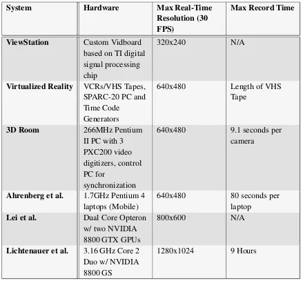
System Hardware Max Real-Time Resolution (30 FPS)

Max Record Time

ViewStation Custom Vidboard

based on TI digital signal processing chip

320x240 N/A

Virtualized Reality VCRs/VHS Tapes,

SPARC-20 PC and Time Code

Generators

640x480 Length of VHS Tape

3D Room 266MHz Pentium

II PC with 3 PXC200 video digitizers, control PC for

synchronization

640x480 9.1 seconds per camera

Ahrenberg et al. 1.7GHz Pentium 4

laptops (Mobile)

640x480 80 seconds per laptop

Lei et al. Dual Core Opteron

w/ two NVIDIA 8800 GTX GPUs

800x600 N/A

Lichtenauer et al. 3.16 GHz Core 2

Duo w/ NVIDIA 8800 GS

[image:27.612.91.527.87.494.2]

1280x1024 9 Hours

Table 3.3: Video Capture Solutions - Summary of Features

3.2 Wireless Sensor Networks

(28)

along with video and audio sensors to make the system more aware of its en-vironment. While the majority of these sensors have analog signals, the data can be digitized and accessed on common PCs through input/output (I/O) boards or analog-to-digital converter (ADC) cards. For example, Phidgets Inc.[22] sells USB sensors along with I/O boards to connect generic analog and digital sensors. They also provide software development kits (SDKs) for most of the common programming languages to access the converted data programmatically.

(29)

Chapter 4 Methodology

The concept for this project originally began as a prototype for an embedded system. The goal was to develop a small, low-power video capture system, that could capture two video streams, do some basic processing, and store the streams, after compressing them, to disk. One of the biggest challenges with designing an embedded system is the cost in terms of time and money for the design phase. Designing a fully custom hardware solution requires thousands of man-hours and many areas of expertise. In addition it is highly unlikely that a custom design will work as expected on the first try. Tracking down problems with custom designs requires significant time for debugging and re-fabrication.

Given the time and budget constraints it was impractical to develop a full custom solution to capture data; instead development boards were explored. There are several companies that manufacture and sell low cost develop-ment boards such as the LeopardBoard[10], BeagleBoard[6] and more re-cently the PandaBoard[42], but these demo boards have a few limitations. These boards often fail to fully utilize the embedded processor they contain, have limited community based support and are generally not designed using production-ready processes.

(30)

4.1 Initial Prototype

[image:30.612.171.447.382.655.2]

The LeopardBoard was chosen for the initial prototype due to it support-ing most of the features that were required and its low cost. The board had several crucial features: board hardware video compression, on-board VGA camera interface, several general purpose pins and ran a cus-tom light-weight OpenEmbedded Linux provided by RidgeRun. While the PandaBoard would have been preferred it was unavailable at the time these experiments were done. Since the LeopardBoard ran a full linux kernel on an ARM chip it was possible to leverage the GStreamer open source mul-timedia framework. The framework uses a pipeline based setup where the source media is piped through various filters/plugins. A basic pipeline for capturing video data at 30 FPS was setup. This pipeline took the source video and compressed it using hardware accelerated MPEG-4 compression (a feature of the processor on the LeopardBoard) and then output to a quick-time .mp4 file.

(31)

Unfortunately one limitation of the board was that it contained only a sin-gle USB port so only one camera source could be interfaced easily. There was a camera interface port, but that required custom hardware design or a pre-manufactured camera board from Leopard Imaging Inc. While the pipeline worked quite well, the hardware itself had problems. The system would inexplicably reset and the replacement board that was received also became faulty within a few days. Due to these reasons a more generic solu-tion was derived. It was important that the new solusolu-tion be easy to maintain and flexible so that additional sensors, other than audio and video, could be handled. Also the solution needed to be low-cost so that it would be cost-effective to build a network of capture systems. From these requirements it was determined that a PC based solution would be best.

4.2 PC Based Solution

Switching to a PC based solution required the choice of an operating system between Windows, Linux/Unix and OSX. Choosing an operating system was not a trivial task because the choices affect the computer hardware to use along with compatible peripheral devices. Determining which to use was decided by several factors which are listed in the table below.

Windows Linux Mac OSX

% of Global Users[46] 86.5 5.9 7.3

3rd Party Device Support High Medium Medium-Low

Media APIs DirectShow GStreamer Quicktime

Familiarity High Medium Low

Hardware Support Medium High Low

Table 4.1: Operating System Comparisons

(32)

the market and most familiar to users. Finally Windows runs on almost any hardware excluding ARM based chipsets and has significant device driver support. Linux is the next closest since it can run on systems that Windows runs on as well as ARM based hardware. OSX has the least hardware sup-port since it can only be used with Apple designed hardware. Windows was chosen over Linux due to the researcher’s own familiarity and experience with the DirectShow and Windows APIs. This system could most likely be ported using Linux and GStreamer in the future for greater hardware sup-port.

The proposed framework consists of:

• Capture Devices

– Hardware

∗ Netbook/Laptop/Tablet PC

∗ Various sensors (analog/digital audio/video sources, Phidget

sensors, GPS sensor)

– Software

∗ User Interface

· Video Preview

· System Status

· Recording Controls

· PhidgetSpatial Interface

· Upload Recordings

∗ DirectShow Filters

· Audio/Video Capture Filter

· PhidgetSpatial Capture Filter

· GPS Capture Filter

· Video Stacking Filter

· Image Processing Filter

· MJPEG Compression Filter

· Video Streaming Filter

· AVI Mux/File Writer Filters

(33)

– Hardware

∗ Desktop PC/Powerful Laptop

– Software

∗ User Interface

· Video Preview - Up to 12 Remote Devices

· Remote Device Control

· Download Recordings

∗ Video Preview

∗ Capture device control, monitor, and archival application

• Wired/Wireless Network

The following sections provide detailed descriptions for each of the items listed above.

4.3 Data Capture - Hardware

Netbooks, slates, and tablet PCs were identified as target platforms for the capture hardware, but desktops could be used if greater real-time processing capabilities are needed.

4.3.1 Computer Platform

(34)

Figure 4.2: ExoPC[12]

(35)

Figure 4.3: Fujitsu LifeBook TH700[15]

(36)

Figure 4.4: 13” MacBook Pro - Windows 7[43]

ExoPC Slate Fujitsu LifeBook

TH700

13” MacBook Pro (Mid 2009)

Processor 1.66 GHz Intel

Atom N450

2.26 GHz Intel Core i3-350m

2.26 GHz Intel Core 2 Duo

Graphics Card Intel HD Intel HD Geforce 9400m

Hard Drive SanDisk 64GB SSD Corsair C300 SSD 1TB, 7200RPM

Memory 2GB DDR2,

667MHz

4GB DDR3, 1066MHz

Networking Gigabit Ethernet,

802.11 b/g/n

Gigabit Ethernet, 802.11 b/g/n

USB 2 USB 2.0 3 USB 2.0 2 USB 2.0

Battery 3-cell, 5139 mAh 6-cell, 5200 mAh 6-cell, 5046 mAH

Dimensions (in) 11.6 x 7.7 x 0.55 11.69 x 9.17 x 1.54 12.78 x 8.94 x 0.95

Weight (lb.) 2.1 4.2 4.5

(37)

Finally, the desktop PC chosen for monitoring was the HP Pavilion Elite HPE-250F[20], shown in Figure 4.5. The HPE-250F has an Intel Core i7-860 (2.80GHz) Quad-Core processor[24], along with a discrete ATI Radeon HD 5770 graphics card. This system provides significant CPU and GPU computational power which is useful for monitoring and manipulating the received data streams in real-time.

Figure 4.5: HP Pavilion Elite HPE-250F[20]

4.3.2 Data Sources

(38)

Interface Bandwidth

PCI[49] 133 Mb/s

PCI-Express 1.0[51] 250 Mb/s per lane (max 16 lanes)

PCI-Express 2.0[51] 500 Mb/s per lane (max 16 lanes)

Firewire 400/800[50] 400 Mb/s / 800 Mb/s

USB 1.0[52] 12Mb/s

USB 2.0[52] 480 Mb/s

USB 3.0[52] 5 Gb/s

Table 4.3: Common PC data interfaces and bandwidths.

4.3.2.1 Analog Video Sources

Two analog color video cameras that are 0.55 inches square, and 0.75 inches in depth were chosen. These cameras are small enough that they can be discretely mounted on clothing or equipment that a user of this system is carrying. The outputs from both the cameras are analog video signals in NTSC format, which is a standard that has been around since the 1940s in the United States. In order to interface these cameras to the PC, two XLR8 XtraView USB analog to digital converters [44] were used.

The NTSC [48] format consists of 29.97 interlaced frames of video per second. These frames are converted to 8-bit YCbCr 4:2:2 digital images using the converters. YCbCr is a color-space used to represent the image data, while 4:2:2 represents the chroma sub-sampling. In this case the the horizontal chroma resolution is halved, which reduces the bandwidth of the video signals by one-third with minimal visual difference.

4.3.2.2 Digital Video Sources

(39)

[image:39.612.265.351.247.356.2]

Figure 4.6: Microsoft LifeCam Cinema - 5 MP Sensor[36]

Figure 4.7: Microsoft LifeCam HD-5000 - 4 MP Sensor[37]

These cameras were chosen because they also come with hardware MJPEG video compression capabilities. This is supported at all resolutions from 160x120 to 1280x720 at full 30 FPS. The other advantage of using digital webcams is that they are designed to fully leverage the cameras capabilities using DirectShow. The device driver for these cameras provide a filter for DirectShow which allows control of many camera properties such as expo-sure, focus, and more as seen in Figures 4.8 and 4.9.

4.3.2.3 Additional Sensor Sources

(40)

pre-built user interfaces to visualize the sensor data. This sensor was cho-sen in particular to show the ease of integrating third-party cho-sensors into this system.

Figure 4.8: DirectShow Camera Properties (Page 1) Filter

(41)

Figure 4.10: PhidgetSpatial 3/3/3 Sensor[21]

The GPS sensor chosen for testing was the USGlobalSat BU-353 USB GPS Receiver[45]. This GPS receiver was chosen due to its USB inter-face and small size. The receiver is NMEA[41] compliant which is a com-mon GPS standard. The USB connection acts as a simple serial connection across which the NMEA data is sent. The data rate is quite low, but some processing is necessary to properly translate the GPS data into meaningful longitude/latitude coordinates, and to visualize this data to the user.

(42)

4.4 Capture Devices - Software

4.4.1 User Interface

The application interface has a minimal design in order to facilitate usage as shown in Figure 4.12, below. The interface is designed to run in both horizontal or vertical orientations depending on how the PC is mounted; this option can be toggled through the file menu.

Figure 4.12: Capture Application - Main Screen

4.4.1.1 Application Modes

The application running on the capture device can run in three modes: pre-view, record, and record with preview. In local preview mode data is not stored at all, allowing the user to calibrate the peripheral devices and pre-view the data output. Calibration involves ensuring the cameras are ori-ented properly, and the spatial sensor is properly zeroed. Although data is not stored in preview mode, it is transmitted over the network so that the monitoring side can connect and verify that valid data is being received.

(43)

mode, local monitoring, remote monitoring, and local data storage are en-abled; this mode requires the most resources and reduces the battery life of the capture device. Due to this, in most cases the device is run with local preview disabled after it has been properly calibrated. Each of these modes is easily enabled through the application interface.

4.4.1.2 Controls

To enable preview mode the preview check-box is toggled on. For recording without preview the preview check-box is toggled off, and the start record-ing button is pressed. Finally for recordrecord-ing with preview the preview check-box is toggled on, and the record button is pressed. Users can create new recordings with filenames based on the current date/time, or a custom file name. Once a recording has started it will continue until the battery life is close to empty, or until the user presses stop recording. Also when a user starts a recording the border around the video panel turns red to indicate that a recording is in progress. Finally, from the user interface it is possible to upload the last recorded video, or a directory of videos to the monitor-ing/archiving device.

4.4.1.3 PhidgetSpatial Interface

(44)

Figure 4.13: PhidgetSpatial - User Interface

4.4.1.4 System Status

The user interface also has a panel that shows basic usage statistics of the capture device. The system metrics are collected using the Performance Monitor API provided by Microsoft. It displays the amount of battery life remaining, amount of free disk space, CPU usage and memory usage so that a user can be alerted when system resources are low.

4.4.2 DirectShow - Filters

(45)

from a video capture card, transform filters are used to modify output from a previous filter such as applying an edge detector to the captured video, and lastly renderer filters which are used for displaying video on the screen or for outputting to files.

Figure 4.14: DirectShow API Overview [35]

In addition to this the DirectShow SDK provides developers access to implement their own filters. It is also possible to create programs that can automatically use these filters in the background in order to handle tasks while providing a more user friendly interface.

In the following sections the filters used and created for this framework are described in greater detail.

4.4.2.1 Audio/Video Capture Filter

(46)

[image:46.612.157.463.228.446.2]

filters are provided for audio and video filters since each has its own spe-cific data stream format and options. For example the audio/video analog to digital converter device drivers provides two filters, one for audio and one for video. In the audio filter it is possible to control the master, treble, and bass volumes, along with other options, while in the video filter it is possi-ble to control the frame rate and color-space of the captured video. The raw audio/video can be further processed using other filters.

Figure 4.15: Audio Filter Properties

4.4.2.2 Video Stacking Filter

(47)

[image:47.612.164.456.88.318.2]

Figure 4.16: Video Filter Properties

Once the frames are combined the stream is sent to an output pin of the filter. Multiple instances of this filter can be used in order to combine many video streams together.

4.4.2.3 Image Processing Filter

The image processing filter integrates OpenCV into a DirectShow filter in order to run image processing algorithms on the raw data streams. OpenCV [7] is an open source API originally created by Intel, but currently main-tained as an open source project that has many optimized algorithms for real-time computer vision. Figure 4.17 shows the software APIs provided by OpenCV.

4.4.2.4 MJPEG Compression Filter

(48)

Figure 4.17: OpenCV Overview [7]

[image:48.612.140.478.86.290.2]

(current frame only) compression based on the discrete cosine transform. Each frame is converted to the frequency domain and then quantized to re-move high-frequency information that has a small perceptual effect of the image. The amount of quantization can be controlled through the quality parameter in order to trade-off between picture quality and file size [47]. Since MJPEG is so widely used, there are no issues in viewing the com-pressed videos across multiple platforms. Figure 4.18 describes the MJPEG compression pipeline. For decompression the process is the same, except the inverse functions of each step are applied. The modern successor to the MJPEG codec are the H.264/AVC codecs.

(49)

The H.264 / AVC codecs are based off the MPEG-4 standard and is de-fined as MPEG-4 part 10, which means that it has some additional features that the base MPEG-4 standard does not have. The goal of the H.264 codec was to heavily reduce file sizes by compressing video more effectively. This is done mainly through exhaustive motion estimation algorithms that allow for up to 16 reference frames compared to the one or two traditionally used in the MPEG-4 standard. H.264 also has entropy coding in order to loss-lessly compress data by creating unique codes that can be used to generate the original data. Through these and other techniques, H.264 provides very high compression at the cost of high computational requirements [19]. Fig-ure 4.19 describes the H.264 algorithm pipeline; compared to the JPEG pipeline it is clear that the H.264 algorithm is significantly more complex and requires additional processing power in order to achieve real-time frame rates.

Figure 4.19: H.264 Encoder Overview [19]

Resolution Uncompressed (MB/s) MJPEG (MB/s) H.264 (MB/s)

(50)

Table 4.4 shows the difference in data rates between un-compressed, MJPEG, and H.264 video streams. As the video size doubles, the data rate for uncompressed video quadruples, while for MJPEG compressed video the data rate doubles as the resolution doubles. Finally with H.264 it is hard to predict the data rate due to the motion estimation and other algo-rithms being performed. Due to algorithmic complexity of recent codecs, the MJPEG codec was chosen due to its simplicity, and minimal compu-tational requirements. Three implementations of an MJPEG compression filter were explored: The FFDShow [11] MJPEG Compressor, the Intel Inte-grated Performance Primitives (IPP)[26] based codec and a custom MJPEG compression filter based off of the Microsoft GDI+[34] APIs.

The FFDShow compressor is a generic media decoder/encoder filter that can compress video using many different compression schemes. Its MJPEG compression implementation is single threaded, but offers high performance.

The Intel IPP library is an extensive library of highly optimized func-tions for media and data processing applicafunc-tions including those needed for JPEG/MJPEG compression. The functions are all multi-core ready and take advantage of processor optimizations such as MMX and SSE1-4.

Finally GDI+ is Microsoft’s application programming interface and is the core component for displaying graphical objects. As it is a core Windows component it has been continually maintained and has improved signifi-cantly from Windows XP to Windows 7 due to added hardware acceleration for certain operations. GDI+ provides libraries for storing and manipulating images in memory and these libraries contain an efficient JPEG encoder. This encoder was wrapped in a DirectShow filter to create a full MJPEG compressor.

4.4.2.5 PhidgetSpatial Capture Filter

(51)

has three data streams: acceleration, gyroscopic and compass orientation.

4.4.2.6 GPS Capture Filter

The GPS capture filter takes the NMEA data stream from the GPS device and parses it into a format that is user-readable. Once a GPS-Fix is acquired the filter takes the user-readable data and renders it to the video frame.

4.4.2.7 Video Streaming Filter

The video streaming filter takes the compressed video stream and transmits it across the network to the monitoring/archival device. The filter was de-signed to transport the video frames using either the UDP or TCP protocols. The RTP protocol was used in conjunction with UDP to packetize and re-assemble the video frames. For the TCP implementation, a simple scheme was used to transmit the frames instead of RTP over TCP. The scheme con-sisted of sending the frame length followed by the frame itself. This was done to avoid overheads associated with packetization and reassembly of the frames. The Nagle[38] algorithm was disabled in order to reduce trans-mission delay for real-time video streaming at the expense of bandwidth.

4.4.2.8 AVI Mux/File Writer Filters

(52)

4.4.3 DirectShow - Filter Graphs

DirectShow graphs enable the creation of content pipelines so that data sources and filters can be swapped out as necessary. The API comes with GraphEdit, a graphical program that can be used to easily configure graphs / pipelines that consist of the filters installed on the system.

The basic pipeline for this implementation consists of four main compo-nents. First is a filter that represents the physical device and has both video and audio outputs. The next two filters in the pipeline are the software inter-face to the audio and video outputs from the physical device. Next are the compression filters, which are used to reduce the bandwidth of the incoming data streams, and finally the last component is the storage medium which can be a file, a network stream, or a combination of both. Figure 4.20, be-low, shows the basic outline of this pipeline. If online processing is desired it is usually inserted into the pipeline before the compression filter.

Figure 4.20: Basic DirectShow Graph

4.5 Monitoring Device

(53)

capture devices at the same time. Each device can be further controlled when in focus.

[image:53.612.93.524.314.611.2]

The controls allow a user to stop/start recordings, configure new record-ings, and to start/stop the data preview. To control the devices distributed systems concepts were used. In C#/.NET distributed systems are imple-mented using .NET Remoting objects. This abstracts the interprocess com-munication that separates the remote object from a specific client or server and from a specific mode of communication. This allows either the client or server end to invoke existing commands on both ends, and pass data back and forth across application/system boundaries. Remoting is an efficient way to handle requests especially as the number of networked computers increase.

(54)

Chapter 5 Results and Analysis

In the following section the three systems used for testing are run through common benchmarks to show the raw performance differences between the systems. The systems were all setup with the same build of Windows 7 and all had their respective hardware drivers installed. Each system was updated with the same set of updates, and for the common hardware used, such as the digital USB webcams and the XLR8 USB analog to digital converter, the same driver was installed on each system to keep results consistent.

5.1 Hardware Benchmarks

First two well known synthetic benchmarks, Prime95[3] and wPrime[53], were used to show the baseline performance of the CPUs in the test com-puters. A synthetic benchmark is one designed to push the CPU to the limit, but not necessarily represent world performance. In order to show real-world performance the framework is used in various configurations to ex-amine performance of capturing different types and combinations of data sources.

5.1.1 Synthetic Tests

(55)

[image:55.612.116.505.149.431.2]

to 8192K. The test was first run using a single thread, then if the CPU sup-ported multiple threads the test was re-run using an increasing number of threads until the maximum was reached.

Figure 5.1: Prime95 - 1 Thread - Benchmark Results

The Prime95 benchmark shows that the ExoPC with the Intel Atom pro-cessor is significantly slower. It computed the FFT 10 times slower than the MacBook Pro and the TH700 systems. On all the systems computing the FFT using two threads the time taken was almost halved. Interestingly even though the MacBook Pro and the TH700 processors have the same clock speeds, the processor in the TH700 is slower. Even as the TH700 uses more threads than the MacBook Pro the synthetic results are slower. This could be due to the benchmark being optimized for one or two threads. The next benchmark wPrime is designed to be optimized for higher thread counts.

(56)

[image:56.612.116.506.88.370.2]

Figure 5.2: Prime95 - 2 Threads - Benchmark Results

The wPrime results are closer to what was expected between the Mac-Book Pro and TH700 performance. The TH700 is faster since it has two physical cores and two logical cores due to hyper-threading, while the Mac-Book Pro only has two physical cores without hyper-threading. The ExoPC still remains the slowest due to the Atom processor. It took 3 times longer than the MacBook Pro, and 5 times longer than the TH700 to compute the result. Finally the MacBook Pro took 1.6 times longer than the TH700 to finish the computation.

ExoPC MacBook Pro TH700

(57)

[image:57.612.115.506.86.371.2]

Figure 5.3: Prime95 - 3 and 4 Threads (TH700 Only) - Benchmark Results

5.1.2 Storage I/O Benchmark

The hard drive benchmarks show the maximum read and write speeds of the drives used in the machines. This is important because it represents the maximum amount of data that can be read or written to the disk per second which directly affects how much data can be captured. If the hard drive is not fast enough to handle the input data, then data can be lost. The benchmark was performed using the ATTO Disk Benchmark program. The hard drives were tested by reading/writing a 2.0GB file using various block sizes between 0.5 to 8192 KB. The results that are most important are for the 2K, 4K, and 8K block sizes since those are typical hard drive write block sizes for optimal performance.

(58)

[image:58.612.116.504.87.369.2]

Figure 5.4: ATTO Storage I/O Benchmark

ExoPC had a first generation SSD from SanDisk and had a read rate of 153.3 MB/s and write rate of 72.2 MB/s. Finally the TH700 with its Corsair C300 SSD had a read rate of 222.6 MB/s and write rate of 172.04 MB/s. These results show that even with SSDs there is a huge range of performance, but even the first generation of SSDs perform better than a standard disk drive by a significant amount.

5.1.3 Networking Throughput Benchmark

(59)

Simple file transfer tests were done with the devices and their performance was similar to the devices tested by CNET.

5.1.4 Battery Life Benchmark

The Battery Eater benchmark [33] is a commonly used Windows benchmark to determine the minimum battery life when the computer is under heavy processing loads.

Platform Rated Battery Life Minimum Battery Life (100% load)

ExoPC 4 Hours 2 Hours 41 Minutes

MacBook Pro 5 Hours 1 Hour 42 Minutes

TH700 5 Hours 2 Hours 35 Minutes

Table 5.2: Battery Life Benchmark

This benchmark tests the system by running the CPU at 100%, the GPU at approximately 15-20% and has occasional disk I/O operations. The above battery life figures can be thought of worst case battery life, while the rated battery life is typical achieved when the system is under a light processing load.

5.2 Framework Benchmark

(60)

The CPU and memory usage graphs are presented in box-whisker plot format. The following plots indicate the minimum (bottom whisker), 1st quartile (bottom of the box), median (red line inside the box), 3rd quartile (top of the box) and maximum (top whisker) for each data set. In addi-tion the outliers are plotted as red crosses. The range inside the box covers the 25th to 75th percentile of the data. Both metrics are displayed in this format because CPU and memory usage are rarely static and can fluctuate depending on the operations being performed.

5.2.1 Uncompressed Audio/Video Capture Pipeline

Uncompressed audio/video capture was tested in order to show the necessity of compression as well as the tradeoff between CPU and disk-bound opera-tions. The uncompressed DirectShow pipeline was simply the audio/video device filter connected directly to the AVI Mux and File writer filters. By setting up the graph this way there is minimal CPU usage since the media capture is done by the USB XLR8 XtraView analog to digital converter. The uncompressed I/O rate can be approximated using the following formulas:

U ncompressed= (W idth∗Height∗3∗30Frames)/1048576

YCbCr 4:2:2 Rate= U ncompressed−(U ncompressed/3)

Resolution Hard Drive I/O (MB/s)

160x120 1.09863 320x240 4.39453 640x480 17.57812 800x600 27.46582 1280x720 52.73438 1920x1080 118.6523

Table 5.3: Uncompressed Audio/Video Capture Results

(61)

video can be a big bottleneck. The regular disk drive would be able to sus-tain only three to four 640x480 video streams of data to disk, and only one or two 800x600 streams. It would not be possible to capture uncompressed HD video with a standard disk drive.The other disadvantage of capturing uncompressed video is that most USB 2.0 cameras do not support resolu-tions higher than 640x480 or 720x480 for uncompressed video due to the high bandwidth requirement.

5.2.2 Compressed Analog Media Capture Pipeline

Two configurations were tested for analog media capture. A single video source and a single video source with stereo audio. For each of these config-urations there were three modes: preview, record and record with preview. The DirectShow graph for each of the configurations is shown as well.

5.2.2.1 Single Video Source

The first configuration was a single video source with no audio, compressed with the FFDShow MJPEG compressor at 90% JPEG quality.

Figure 5.5: Single Analog Video Source - Preview Mode - DirectShow Graph

(62)

video preview. The next configuration shown is for recording the analog video output.

Figure 5.6: Single Analog Video Source - Record Mode - DirectShow Graph

For the recording graph, shown in Figure 5.6, it is unnecessary to have the AVI Decompressor and Color Space Converter filters since FFDShow handles those functions internally. So the USB 2821 Video connects directly to the FFDShow Video Encoder which then goes through an AVI Mux filter which is used to interleave audio/video, or in this case just the video into a proper AVI format. Finally a File Writer filter is used to create a valid file on the storage medium. The last configuration graph handles both recording and preview.

Figure 5.7: Single Analog Video Source - Record and Preview Mode - DirectShow Graph

(63)

since the timing of data isn’t as important and increases performance since frames can be dropped as needed. This is especially useful when streaming data over the network since it is preferred to transfer the data as soon as it is available rather than waiting and sending the frames at constant offsets.

[image:63.612.92.524.253.588.2]

For each of the systems these three DirectShow graphs were run at three different resolutions: 160x120, 320x240, 640x480. Resolutions greater than 640x480 were not tested since they were not possible with the analog cam-eras.

Figure 5.8: ExoPC - CPU Usage - Single Analog Video Source

(64)

[image:64.612.91.524.322.661.2]

much more variance in the data. This is due to the lack of multi-threading support and the single processing core of the Atom chip. Contention occurs between the CPU resources so at times the CPU has to wait for resources to be free before performing the compression computations. This is especially apparent at the 640x480 resolutions where the recording and preview mode CPU usage doubles compared to just recording or just previewing. From these results it should be possible to run two analog cameras at 160x120 or 320x240 in real-time while recording and previewing, but additional cam-eras would cause performance to drop below real-time. Additionally these results show that there is room for other sensor data to be captured when the resolution is below 640x480. Unfortunately capturing and compressing a single 640x480 video comes close to maxing out the ExoPC capabilities.

(65)

The MacBook Pro CPU usage is approximately half the amount as the CPU usage of the ExoPC as shown in Figure 5.9. This shows that the Mac-Book Pro could support up to five 160x120, three 320x240, or two 640x480 streams in all modes. However, two 640x480 sources in record with preview mode would maximize the capabilities of the MacBook Pro. It is surprising that the MacBook Pro is only twice as fast as the ExoPC. In the synthetic benchmark wPrime, it was shown that the MacBook Pro raw performance was three times faster than the ExoPC and in the Prime95 benchmark it was ten times as fast. It is clear from this result that real-world performance can be different compared to a simple synthetic test. Interestingly the MacBook Pro CPU performance does not follow the same trend as the ExoPC’s. Here the preview and recording mode take about the same amount of CPU usage for the 160x120 resolution, but the record with preview mode jumps to the same CPU usage as the 320x240 resolution tests; however, the 320x240 re-sults are unexpected as well since all of the modes use approximately the same amount of CPU instead of varying as expected. At the 640x480 res-olution the results for each mode is closer to the expected result, but the preview mode took much less CPU than recording which was unexpected.

(66)

[image:66.612.92.526.97.439.2]

Figure 5.10: TH700 - CPU Usage - Single Analog Video Source

clock speed, the additional logical cores and architectural improvements al-low the TH700 to achieve twice the performance of the MacBook Pro.

5.2.2.2 Single Video and Audio Source

The second configuration was a single video source with a single stereo audio source, compressed with the FFDShow MJPEG compressor at 90% JPEG quality for the video and the LAME MP3 encoder at 128 kbps at 44.1kHz sampling rate for the audio.

(67)

Figure 5.11: Single Analog Video and Audio Source - Preview Mode - DirectShow Graph

The record mode shown in Figure 5.12 has the same video pipeline as in Figure 5.6. For the audio pipeline the USB EMP Audio Device filter represents the audio source, this is attached to the LAME Audio Encoder and piped to the same AVI Mux as the video.

[image:67.612.93.531.90.297.2]

Finally the record with preview mode in Figure 5.13 has the same video pipeline as in Figure 5.7. The audio pipeline the USB EMP Audio Device filter represents the audio source which is connected to a Smart Tee filter. The preview output of the Smart Tee is connected to the Default Direct-Sound Device, while the capture output is attached to the LAME Audio Encoder and piped to the same AVI Mux as the video.

(68)

[image:68.612.92.527.89.318.2]

Figure 5.13: Single Analog Video and Audio Source - Record and Preview Mode - Direct-Show Graph

Figure 5.14 shows that the addition of audio capture increased the CPU usage by 2-4% for the preview mode, while for the recording and record with preview mode the CPU usage increased by 10-20% due to the LAME MP3 audio compressor. This clearly causes an issue at the 640x480 record with preview mode where the CPU usage goes to maximum approximately 25% of the time. For this test case the capture rate of the video dropped to 28.64 frames per second. This shows that the ExoPC can only capture video at 640x480 resolution with audio if it is not being previewed at the same time. The increase in CPU usage is much more dramatic for the ExoPC compared to the other systems due to its single-core processor. There is a significant performance hit since the CPU must first handle the video data then the audio data instead of handling them simultaneously.

(69)

[image:69.612.89.524.97.437.2]

Figure 5.14: ExoPC - CPU Usage - Single Analog Video and Audio Source

resolutions much more video data is captured since there are many more bits for each frame of the video, while audio data rates are quite small. In addition to the audio source the MacBook Pro is capable of capturing up to two 640x480 video sources with some headroom for a low data-rate sensor. Figure 5.16 shows that the addition of the audio stream makes a negligi-ble difference in the overall range of the CPU usage for the TH700. Instead the variance of the CPU usage increased, especially at the 320x240 resolu-tion as seen in Figures 5.10 and 5.16.

(70)

[image:70.612.92.523.92.435.2]

Figure 5.15: Macbook Pro - CPU Usage - Single Analog Video and Audio Source

them more desirable to use in many applications.

5.2.3 Software Compressed Digital Media Capture Pipeline

(71)

Figure 5.16: TH700 - CPU Usage - Single Analog Video and Audio Source

[image:71.612.92.525.95.436.2]

The first configuration was a single digital video source with no audio, com-pressed with the FFDShow MJPEG compressor at 90% JPEG quality.

Figure 5.17: Single Digital Video Source - Preview Mode - DirectShow Graph

(72)

shown in Figure 5.17. For the video pipeline it was no longer necessary to include a Color Space Converter filter from the video source, but an AVI decompressor was still necessary since the video stream was still transmitted as an AVI stream. Finally the decompressed AVI stream was connected to the Video Mixing Renderer filter to display the video on the screen.

Figure 5.18: Single Digital Video Source - Record Mode - DirectShow Graph

For the recording mode in Figure 5.18 the LifeCam Cinema filter was connected to the FFDShow Video Encoder, which was connected to an AVI Mux and a File Writer filter. This is exactly the same workflow as for the analog case seen in Figure 5.6.

Figure 5.19: Single Digital Video Source - Record and Preview Mode - DirectShow Graph

(73)

[image:73.612.91.523.178.516.2]

graphs were run at three different resolutions: 160x120, 320x240, 640x480. Resolutions greater than 640x480 were not tested since the digital cameras did not support higher resolutions at 30 FPS when capturing uncompressed streams.

Figure 5.20: ExoPC - CPU Usage - Single Digital Video Source

(74)

[image:74.612.91.523.127.464.2]

single 640x480 video comes close to maxing out the ExoPC capabilities.

Figure 5.21: Macbook Pro - CPU Usage - Single Digital Video Source

Digital video capture on the MacBook Pro was significantly faster than analog capture at all resolutions, which can be seen from Figures 5.21 and 5.9. At 160x120 resolution the CPU usage was approximately 5-8% less, and 10-15% less at 320x240 and 640x480. In addition while the variance remained about the same as the analog capture, the median decreased sig-nificantly in all cases. This shows that the average CPU usage was lower than in the analog capture. In this configuration it would be possible to cap-ture up to ten 160x120, five 320x240, or three 640x480 video sources in real-time. The gains seen with the MacBook Pro were not expected.

(75)

[image:75.612.91.527.94.438.2]

Figure 5.22: TH700 - CPU Usage - Single Digital Video Source

seen in the ExoPC, where performance did not improve using digital sen-sors. The performance scaling of the TH700 remains the same as in the analog case such that up to nine 160x120, six 320x240 or four 640x480 video sources could be captured.

5.2.3.2 Single Video and Audio Source

The second configuration was a single video source, compressed with the FFDShow MJPEG compressor at 90% JPEG quality along with a stereo au-dio source compressed with the LAME MP3 encoder at 128 kbps at 44.1kHz sampling rate.

(76)

Figure 5.23: Single Digital Video and Audio Source - Preview Mode - DirectShow Graph

5.23, has the same video pipeline as in Figure 5.17. For the audio pipeline the Desktop Microphone filter represents the digital audio source, this is attached directly to the Default DirectSound Device which renders the audio to the default speakers that are active.

Figure 5.24: Single Digital Video and Audio Source - Record Mode - DirectShow Graph

In record mode the graph in Figure 5.24 has the same video pipeline as in Figure 5.18. For the audio pipeline the Desktop Microphone filter represents the digital audio source, this is attached to the LAME Audio Encoder and piped to the same AVI Mux as the video.

Finally the record with preview mode graph seen in Figure 5.25 has the same video pipeline as in Figure 5.19. The Desktop Microphone filter repre-sents the digital audio source which is connected to a Smart Tee filter. The preview output of the Smart Tee is connected to the Default DirectSound Device, while the capture output is attached to the LAME Audio Encoder and piped to the same AVI Mux as the video.

(77)

[image:77.612.92.524.280.618.2]

Figure 5.25: Single Digital Video and Audio Source - Record and Preview Mode - Direct-Show Graph

Figure 5.26: ExoPC - CPU Usage - Single Digital Video and Audio Source

(78)

[image:78.612.91.523.251.591.2]

capture capabilities of the ExoPC so that only two 160x120 video sources or single 320x240/640x480 source could be captured in conjunction with an audio source. Comparing this result to the analog video and audio capture setup, it can be seen by comparing Figure 5.14 to the figure above that the digital capture pipeline is more efficient by 2-5% less CPU usage. In the analog 640x480 record with preview mode test the system maxed out the CPU and failed to achieve a full real-time frame-rate, but the digital capture remained under 90% CPU usage leaving room for additional tasks.

Figure 5.27: MacBook Pro - CPU Usage - Single Digital Video and Audio Source

(79)

[image:79.612.91.523.159.499.2]

this setup in Figure 5.15 it can be seen that the performance of the digital version is significantly faster with 10-20% less CPU usage across the test cases.

Figure 5.28: TH700 - CPU Usage - Single Digital Video and Audio Source

(80)

5.2.3.3 Dual Video Source

The final configuration was two digital video sources with no audio, each compressed with the FFDShow MJPEG compressor at 90% JPEG quality. The capture pipeline for the modes shown in Figures 5.29, 5.30, and 5.31 is identical to the setup for a single digital video source per video source as seen in Figures 5.17, 5.18 and 5.19.

Figure 5.29: Dual Digital Video Source - Preview Mode - DirectShow Graph

Figure 5.30: Dual Digital Video Source - Record Mode - DirectShow Graph

For each of the systems these three DirectShow graphs were run at three different resolutions: 160x120, 320x240, 640x480. Resolutions greater than 640x480 were not tested since the digital cameras did not support higher resolutions at 30 FPS when capturing uncompressed streams.

(81)

[image:81.612.87.523.272.609.2]

Figure 5.31: Dual Digital Video Source - Record and Preview Mode - DirectShow Graph

Figure 5.32: ExoPC - CPU Usage - Dual Digital Video Source

(82)

sensor data.

Figure 5.33: MacBook Pro - CPU Usage - Dual Digital Video Source

On the MacBook Pro, capturing two digital video streams approximately doubles the CPU usage in all modes as shown in Figure 5.33. This verifies that in this configuration it would be possible to capture up to ten 160x120, five 320x240, or three 640x480 video sources in real-time as stated for the single digital video stream.

(83)

5.2.4 HW Compressed Digital Media Capture Pipeline

Only two configurations were tested for digital capture with hardware video compression. A single video source and a dual video source configura-tion. For each of these configurations there were three modes: preview, record and record with preview. The DirectShow graph for each of the con-figurations is shown as well. These concon-figurations used hardware MJPEG compression in order to show the benefits/disadvantages of hardware accel-eration.

(84)

In preview mode since the output of the video source is already an MJPEG stream, the stream needs to be decompressed. This was done using the MJPEG Decompressor filter that comes default with Windows. This was then connected to the Video Mixing Renderer filter to render the video to the screen as shown in Figure 5.35. For recording mode the MJPEG stream from the video source can be directly output to an AVI file so no interme-diate filters are needed, shown in Figure 5.36. Finally for the record and preview mode the above configurations are combined into a single pipeline as shown in Figure 5.37. These graphs were only tested at 800x600 and 1280x720 resolutions since it was known that the systems could handle lesser resolutions with software compression, so with hardware compres-sion the performance would be significantly faster.

Using hardware compressed video capture the ExoPC had no trouble capturing video up to 1280x720 resolution as shown in Figure 5.38. The preview modes took significantly more CPU usage than the record modes because of the software decompression of the video stream for display. In the record mode the CPU usage for both resolutions was identical. This was expected because the stream is being compressed within the video sen-sor device. The CPU usage for the single hardware compressed 1280x720 stream was approximately 20-30%, using software compression this was the amount of CPU needed for a single 640x480 stream. From this result it would be possible to capture up to three 1280x720 video streams with-out preview, or three 800x600 video streams while previewing one of the streams.

Figure 5.39 shows that the MacBook Pro was able to capture 800x600 and 1280x720 resolution hardware compressed video using less than 10%

(85)

Figure 5.36: Single Digital Video Source - Record Mode - Hardware Compression - Di-rectShow Graph

Figure 5.37: Single Digital Video Source - Record and Preview Mode - Hardware Com-pression - DirectShow Graph

of the CPU in the record mode. This means that it is possible to capture up to ten 800x600 or 1280x720 video streams on this system. For preview modes it should be possible to preview and capture one to two 800x600 streams. Oddly the 1280x720 preview mode performance was much bet-ter than previewing the 800x600 streams. It is unknown why the perfor-mance was better at 1280x720 resolution. It is possible that the Geforce 9400m graphics card was accelerating streams of certain resolutions such as 1280x720 which is a standard HD video resolution. From these results it should be possible to preview and capture up to three 1280x720 streams.

(86)

Figure 5.38: ExoPC - CPU Usage - Single Digital Video - Hardware Compressed

could capture up to twelve 800x600 and ten 1280x720 video streams.

5.2.4.2 Dual Video Source

(87)

Figure 5.39: MacBook Pro - CPU Usage - Single Digital Video Source - Hardware Com-pressed

Capturing two hardware compressed sources was possible for the Ex-oPC, but only during record only mode as shown in Figure 5.41. Preview-ing the video streams in real-time was not possible. While the record mode suggests that the CPU usage was 20-30%; however, there were a significant number of outliers. Based on the single video capture it was expected that the overall CPU usage would be around 60% for capturing two streams.