Detailed flow measurement of the field around tidal turbines with and without biomimetic leading-edge tubercles

(1)

1

Detailed flow measurement of the field around tidal turbines

1

with and without biomimetic leading-edge tubercles

2 3

Weichao Shi 1,2_{, Mehmet Atlar}2_{, Rosemary Norman}1

4 5

1 School of Marine Science and Technology, Newcastle University, UK 6

2 Department of Naval Architecture, Ocean & Marine Engineering, University of Strathclyde, 7

UK 8 9 10

Corresponding Author 11

Weichao Shi, w.shi6@ncl.ac.uk 12

School of Marine Science & Technology, Armstrong Building, Newcastle University 13

United Kingdom, NE1 7RU 14

Tel: 0044 (0)191 222 5067 15

Fax: 0044 (0)191 222 5491 16

(2)

2

Abstract: This paper focuses on implementing detailed flow measurement using advanced 19

Particle Image Velocimetry (PIV) system to investigate the flow mechanism of leading-edge 20

tubercles on tidal turbine blades. Two approaches have been applied: one is 2D PIV to map 21

the flow separation around the blade sections at different radial positions; and the other is 22

Stereo PIV to conduct a volumetric measurement in the wake field to reveal the tip vortex 23

development and also velocity distribution. The research presented in this paper further 24

demonstrates that the leading-edge tubercles can enable the flow to remain attached to the 25

blades and weaken the three dimensional effect which can lead to efficiency loss or the so-26

called “tip loss”. Based on these phenomena that have been observed and concluded from 27

the tests, the mechanism by which leading-edge tubercles can provide additional torque and 28

thrust for a tidal turbine has been explained within this paper. 29

Keywords: Particle Image Velocimetry (PIV), Tidal turbine, Blade design, Tubercles, 30

Biomimetic 31

(3)

3

1 Introduction

33

Flow control devices have been widely adopted to stimulate the performance of foils and 34

related devices; these include leading-edge slats, trail-edge flaps, winglets and vortex 35

generators, etc. However recently a biomimetic concept, the leading-edge tubercles on the 36

pectoral fins of humpback whales, has drawn attention [1, 2]. The tubercles first 37

demonstrated a delayed stall and also enhanced lift-to-drag ratios in an investigation in wind 38

tunnel tests for a pair of replica humpback whale flippers with and without leading-edge 39

tubercles [3, 4]. Following this, investigations both numerical and experimental in nature, 40

have looked at potential applications of leading-edge tubercles applied to air fans, wind 41

turbines, rudders, propellers and so on [5-10]. 42

Following a pioneering study that applied tubercles to a tidal turbine [11], recently the team 43

in the Emerson Cavitation Tunnel (ECT), Newcastle University has initiated a new blade design 44

study, by applying the concept to a tidal turbine [12-14]. Initially a study was conducted into 45

a 3D hydrofoil with a tidal turbine chord length distribution but a constant pitch angle, which 46

demonstrated the increased lift after the stall angle and the enhanced maximum lift-to-drag 47

ratio [12]. Using computational fluid dynamics analysis, it was also shown that the three 48

dimensional effect, which causes spanwise flow, can be reduced by the contra rotating vortex 49

fence generated by the tubercles [15]. 50

With confidence built from the hydrofoil study, the design was applied to a scaled turbine 51

model with different levels of tubercle coverage. The scaled model tests were conducted for 52

a number of different purposes, including hydrodynamic performance analysis, cavitation 53

observation and noise performance. It has been proved that the hydrodynamic performance 54

of the turbine can be enhanced in the low tip speed ratio region without lowering the 55

maximum power coefficient, which will enable the turbine to start at lower flow velocities 56

[13]. The tubercles can also help in restraining the cavitation region and hence lowering the 57

noise level [14]. With these benefits, a quiet and quick reacting turbine design can be 58

established. 59

However, the reasons why such benefits can be introduced by this tubercle concept have 60

been discussed and argued by many researchers but not conclusively; these arguments 61

include compartmentalization, vortex lift, varying the effective angle of attack and boundary 62

layer momentum exchange [6]. Therefore, to further investigate the flow mechanism behind 63

the tubercle function, a set of detailed flow measurements have been conducted. The test 64

setup and results are presented and discussed in the following sections. Particle Image 65

Velocimetry (PIV) technology was used to measure the velocity distribution and two different 66

setups were employed, one for mapping of the flow separation and the other one for 67

(4)

4

2 Description of the tested model

69

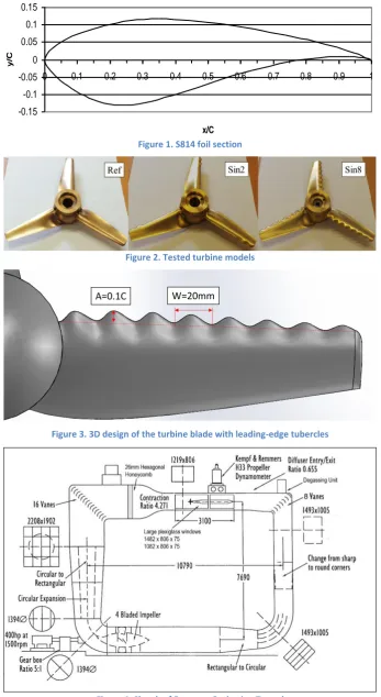
The reference turbine was chosen to be a model that was designed, tested and numerically 70

modelled during a previous project [16, 17]. Based on this model, leading-edge tubercles were 71

applied to the blades. The blade section of the reference turbine used the NREL S814 foil 72

section, as shown in Figure 1. The main particulars for this 400mm diameter model turbine 73

are shown in Table 1. 74

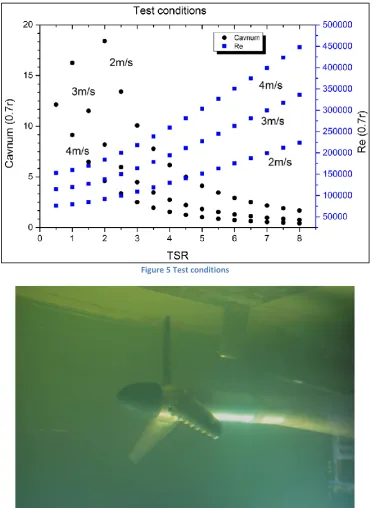
Three pitch-adjustable turbine models with different leading-edge profiles were 75

manufactured by Centrum Techniki Okrętowej S.A. (CTO, Gdansk), as shown in Figure 2. “Ref” 76

refers to the turbine model with a smooth leading edge; while “Sin2” refers to the one with 77

two leading-edge tubercles at the tip; and the one with eight leading-edge tubercles is named 78

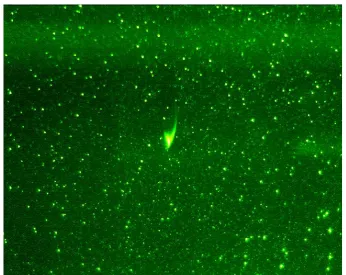
“Sin8”. The sinusoidal leading-edge profile was developed as shown in Figure 3. The 79

amplitude (A) of the sinusoidal tubercles was equal to 10% of the local chord length (C) while 80

eight tubercles were evenly distributed along the radius with the wavelength (W) equal to 81

20mm. The profile of the leading tubercles was as represented by Equation 1. 82

𝐻 =𝐴 2𝑐𝑜𝑠 [

2𝜋

𝑊 (𝑟 − 40) − 𝜋] + 𝐴 2

Equation 1

Where H is the height of the leading-edge profile relative to the reference one which is the 83

smooth leading-edge profile. 84

3 Experimental setup and approach

85

3.1 Description of the Emerson Cavitation Tunnel

86

The three tidal turbine models were tested in the Emerson Cavitation Tunnel (ECT) at 87

Newcastle University. A sketch of the tunnel is shown in Figure 4. The tunnel is a medium size 88

propeller cavitation tunnel with a measuring section of 1219mm × 806mm (width × height). 89

The speed of the tunnel water varies between 0.5 and 8 m/s. Full details of the ECT can be 90

found in [18]. 91

3.2 Turbine control and force measurement

92

The turbine was mounted on a vertically driven dynamometer, Kempf & Remmers H33, 93

designed to measure the thrust and torque of a propeller or turbine. A 64kW DC motor is 94

mounted on top of the dynamometer to control the rotational speed of the turbine. The setup 95

is shown in Figure 6. 96

The rotational speed is controlled by the motor to achieve the desired Tip Speed Ratio (TSR) 97

which can be calculated using Equation 2. During the model tests, the torque and thrust of 98

the turbine were measured and from these measurements the power coefficient (Cp) and the 99

thrust coefficient (CT) can be derived by using Equation 3 and Equation 4 respectively:

(5)

5

𝑇𝑆𝑅 =𝜔𝑟 𝑉

Equation 2

𝐶𝑝 =₁ 𝑄𝜔 2 𝜌𝐴𝑇𝑉3

Equation 3

𝐶_𝑇 =₁ 𝑇 2 𝜌𝐴𝑇𝑉2

Equation 4

where Q is the torque of the turbine, in Nm; T is the thrust, in N; 𝜔 is the rotational speed, in 101

rad/s; AT is the swept area of the turbine and equals D2/4, m2; 𝜌 is the tunnel water density,

102

in kg/m3_{; V is the incoming velocity, in m/s, D is the turbine diameter, in m.}

103

As the performance of the turbine is strongly dependent on the Reynolds number and the 104

cavitation number, these two non-dimensional numbers at 0.7 radius of the turbine blade, 105

𝑅𝑒_0.7𝑟 and 𝐶𝑎𝑣0.7𝑟 were monitored and can be derived from Equation 5 and Equation 6

106

respectively. 107

𝑅𝑒0.7𝑟 =

𝐶_0.7𝑟√(𝑉2_{+ (0.7𝜔𝑟)}2 ν

Equation 5

𝐶𝑎𝑣_0.7𝑟 = ₁ 𝑃0.7𝑟− 𝑃𝑣 2 𝜌√(𝑉2+ (0.7𝜔𝑟)2

Equation 6

where 𝐶0.7𝑟is the chord length of the turbine at 0.7 radius, m; ν is the kinematic viscosity of

108

the water, m²/s; 𝑃0.7𝑟 is the static pressure at the upper 0.7 radius of the turbine, Pa; 𝑃𝑣 is the

109

vapour pressure of the water, Pa. 110

Throughout the test campaign, the incoming flow velocity of the tunnel was fixed and the 111

rotational speed was varied to achieve the required TSR. The tests were conducted according 112

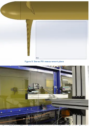
to the test matrix shown in Table 2. The test conditions are also shown in graphical format in 113

Figure 5. At high Reynolds numbers, due to the increased incoming velocity, cavitation 114

number was reduced and hence cavitation might occur at the turbine blades. Taking 115

advantage of the pitch adjustable design, three different pitch angles of the turbine blades 116

were tested. Details of the hydrodynamic performance, cavitation observation and noise 117

measurement, have been presented in the papers [13, 14]. 118

(6)

6

3.3 2D/ Stereo PIV system and calibration

120

The PIV system used in the ECT is a Dantec Dynamics Ltd system and a summary of its 121

technical details is given in Table 3. In this test, both 2D PIV and SPIV measurements were 122

conducted. 123

3.3.1 Setup of 2D PIV 124

Within this experiment, 2D PIV measurement was carried out for the purpose of measuring 125

the velocity distribution within the planar sections at different radii, as shown in Figure 7. The 126

two dimensional velocity vector in the plane can be measured in this way. The flow separation 127

area can be mapped and compared after the test so that the differences of flow separation 128

influenced by the leading-edge tubercles can be revealed. 129

The flow field was illuminated by the laser system and the highly seeded flow field was filmed 130

using a high-speed CCD camera which was set perpendicular to the light sheet. A sample 131

image is shown in Figure 8. 132

3.3.2 Setup of Stereo PIV 133

Following the 2D PIV measurement, a stereo PIV measurement was conducted to measure 134

the three velocity components in a plane after the turbine. The measurement plane of the 135

SPIV is shown in Figure 9. 136

The stereo PIV used the same laser system to illuminate the seeded flow field. However two 137

high-speed cameras were used to capture the image from different angles. The setup of the 138

Stereo PIV system in the ECT is shown in Figure 10. Typical images from the two cameras are 139

shown in Figure 11. 140

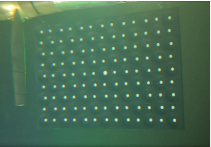
The use of the SPIV needs special calibration for the two cameras, which involves a multi-level 141

270x190mm calibration target. In order to calibrate the SPIV system, the calibration target 142

had to be installed in the measurement plane, as shown in Figure 12. The two cameras viewed 143

the calibration target from the same side but different angles. The calibration result is shown 144

in Figure 13, which also shows the camera positions. 145

3.4 Phase averaging and Image processing

146

Throughout the measurements of 2D PIV and stereo PIV, 100 double frame image pairs 147

needed to be captured, analysed and averaged to achieve a time-averaged velocity 148

distribution. In order to capture these images always at the same azimuth position of the 149

turbine, the camera and the laser were controlled and synchronized by a cyclic synchronizer. 150

This cyclic synchronizer is based on an encoder on the motor and a CompactDAQ system from 151

National Instruments coded in LabVIEW, which has the capability of triggering the camera at 152

the desired angular positions. However, the rotational rate of the turbine needed to have a 153

minimum value of 350rpm to enable the system. 154

In order to analyse the images and hence to determine the flow velocities, adaptive PIV 155

analysis was used for the 2D images from each camera. Afterwards, the results of these 100 156

(7)

7

calibration results and the 2D PIV data, finally the SPIV results with three component velocity 158

could be achieved, as shown in Figure 14, and also the detailed structure of the tip vortex 159

could be revealed. 160

4 Testing conditions

161

Based on the hydrodynamic performance tests, the performance of the three turbines at 162

three different pitch angles, 0⁰, +4⁰ and +8⁰, was evaluated in the first stage, which provided 163

the guidelines for the PIV measurement. According to the test result at 2m/s, shown in Figure 164

15 , even though +8⁰ pitch angle has a slightly lower power coefficient (Cp) compared to +4⁰, 165

it has much lower thrust (CT/10) and also a better starting performance in the lower range of

166

TSRs. Therefore the +8⁰ pitch angle was selected to be investigated in this paper for the PIV 167

test. 168

The PIV test was conducted at three different TSRs in order to thoroughly understand the 169

effect caused by the leading-edge tubercles while the turbine was operating under different 170

conditions. This test needed to consider not only the minimum RPM requirement but also the 171

impact of blade cavitation, since cavitation bubbles could greatly deteriorate the image 172

quality. Therefore, the following three typical working conditions were selected. 173

1. Stall condition (TSR=2): Tidal turbine will experience this condition while accelerating 174

up to the optimum working condition (TSR=4). However under this stall condition, 175

flow separation could occur. The most significant improvement resulting from the 176

leading-edge tubercles has been found under this condition. During the test, an 177

incoming velocity of 4m/s and a rotational speed of 382rpm were used. The 178

performance comparison of Cp and CT/10 is presented in Table 4.

179

2. Optimum working condition (TSR=4): This is the optimum condition under which the 180

turbine would operate in order to maximise the power generation. This is also the 181

turbine’s design condition. Most turbines will maintain this TSR to achieve the 182

maximum power coefficient. During the test, an incoming velocity of 3m/s and 183

rotational speed of 573rpm were set. 184

3. Overspeed condition (TSR=5): This is the condition in which the turbine is working 185

beyond the optimum TSR. This is often considered to be the overspeed condition that 186

might be harmful for the generator and gearbox. However there are some turbines 187

designed to operate under this condition since the higher rotational speed will result 188

in better generator performance. More stable performance can be expected 189

compared to the optimum working conditions under which the turbine might suffer 190

from stall due to the natural flow fluctuation caused by waves or turbulence. During 191

the test, an incoming velocity of 3m/s and rotational speed of 716rpm were set. 192

The performance comparison of the above three conditions has been summarised in Table 4. 193

It can be noticed that at high TSR the increment in Cp for the turbine with tubercles is related 194

to a rather significant increase in CT. While at TSR=2, the increase in Cp is much higher than

195

the increase in CT, with the increase of TSR the inflow angle will be reduced inducing more

196

thrust while with the decrease of TSR the opposite will be true for the inflow angle, i.e. 197

(8)

8

5 Result analysis

199

5.1 Visualizing the planar section using 2D PIV

200

For the purpose of mapping the flow separation region around the turbine blade, 2D PIV 201

measurement was conducted for the above three turbines in the selected three typical 202

conditions. All of the cases are referred to in the form “Model_Velocity_TSR_Position”, i.e. 203

“Ref_4_TSR2_0.95R”. 204

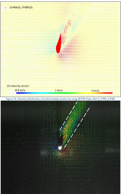
The measurement result of 2D velocity distribution of the reference turbine at 0.95r under 205

4m/s with TSR=2 is presented in Figure 16 with the reference vector (U=4m/s, V=0m/s) 206

displayed at the top left corner. It shows typical flow separation behind the turbine blades. 207

However, in order to highlight the flow separation area behind the blade, the following results 208

are presented in a form shown in Figure 17 with the reference vector being subtracted and 209

the actual image being plotted in the background. As it can be seen, the turbine is suffering 210

from significant flow separation after the blade, as marked between the white dashed lines. 211

With this methodology, the flow separation area can be clearly mapped and compared. 212

All of the measurement results under TSR=2 are presented using the above method, as shown 213

in Table 5. In order to clearly compare the flow separation area, the vorticity Z distribution is 214

plotted in Table 6. In-depth analysis and a comparison between the performance of the three 215

different turbines is shown in Table 4 indicating the dramatic difference in the stall condition, 216

under which the flow around the turbine is also significantly changed by the tubercles. It can 217

be clearly seen in Table 5 that the leading-edge tubercles can help the flow to be more 218

attached to the turbine blade at various radial positions particularly from 0.8R to 0.95R. This 219

phenomenon has proved the beneficial effect of the leading-edge tubercles for tidal turbines, 220

especially under the stall condition is because of the more attached flow. 221

At sections towards the hub, the flow separation is gradually reduced due to the decreasing 222

angle of attack. However the flow separation observed in the mid span region of the Sin8 223

turbine blades might be slightly larger from 0.6R to 0.45R as the result of the change in the 224

angle of attack. This is because, at this region, the tubercles operating at unfavourable angles 225

of attack and triggering a leading-edge flow separation due to the high speed flow induced by 226

the tubercles. In contrast the reference turbine without tubercles will generate trailing-edge 227

flow separation. 228

For the other two conditions, TSR=4 and TSR=5, the flow separation phenomenon has not 229

been clearly observed since the angles of attack are lower than the stall angle; therefore the 230

measurement results have been presented as a database for future research in Appendix A, 231

Table 7 at TSR=4 and Table 8 at TSR=5. 232

5.2 Mapping the volumetric flow field using SPIV

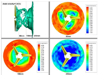
233

By using SPIV, three velocity components: the axial velocity, the radial velocity and the 234

tangential velocity can be visualised in the measuring plane downstream of the turbine blades 235

along with the resultant vorticity distribution. With the aid of the phase locking and averaging 236

technique discussed in Section 3.4, SPIV measurements were conducted every 10° of angular 237

(9)

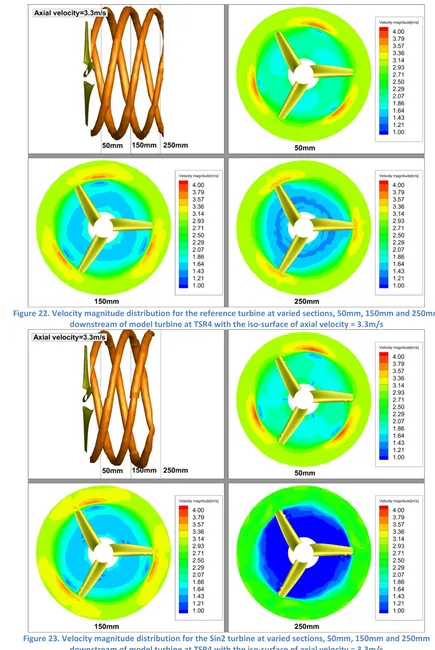
9

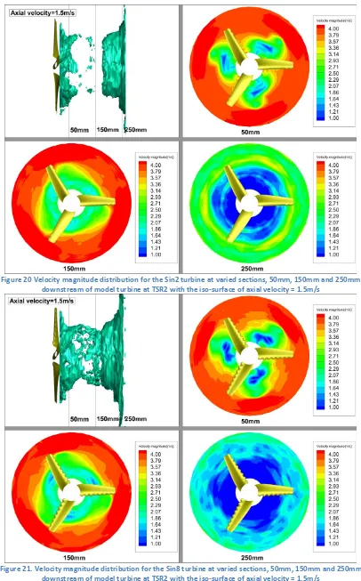
different positions, a volumetric flow field can be achieved to resolve the turbine’s wake field, 239

as shown in Figure 18. In Figure 19 to Figure 27, the velocity magnitude distributions in the 240

wake field downstream of these three different turbines under various conditions have been 241

presented. In the following sections, detailed analysis and discussion are presented with 242

regard to each of the individual conditions. Three sections, which are consecutively 50mm, 243

150mm and 250mm downstream of the turbine, were extracted and the velocity magnitude 244

plotted at those sections. 245

5.2.1 Condition 1: Stall condition, TSR=2 246

In Figure 19 to Figure 21, the velocity magnitude distribution under the stall condition has 247

been presented together with the iso-surface of axial velocity=1.5m/s. As discussed in Section 248

5.1, severe flow separation occurred under this condition. Because of the flow separation that 249

the turbines suffered, in the wake field the flow is much more turbulent compared to the 250

other conditions. Also, because of the low tip speed ratio, the tip vortex structure is not very 251

clearly seen from the iso-surface. 252

It can be noticed that the tail of iso-surface plot for the Sin2 case is slightly behind the other 253

two turbine cases and the associated iso-surface appears to be more intermittent compared 254

to the other two cases and this results in a significant difference at section d=250mm. This is 255

because of the fact that the flow is mixed quicker and hence the velocity deficit in the mid-256

span can be recovered faster by the Sin2 turbine compared to other two turbine cases. It can 257

also be seen for section d=150mm the flow of Sin2 in the mid-span region has a higher speed 258

compared to the other two turbine cases. 259

By extracting the iso-surface pair of radial velocity= +/-0.5m/s in Figure 28, the tip vortex can 260

be revealed which is rolling from the pressure side to the suction side and disappearing in the 261

wake. The iso-surface for the turbine Ref is wider and smoother than that for the other two 262

turbines. For the case Sin8 especially, the iso-surface is quite narrow but extends for a longer 263

distance. This trend can also be seen in which shows the iso-surface of the vorticity (tangential) 264

= 100. This component of vorticity results from the axial velocity and the radial velocity and 265

also reveals the tip vortex. As it can be seen, the iso-surface of the Sin8 case is longer but 266

narrower. This indicates that the tip vortex of the turbines with tubercles under the stall 267

condition is stronger but cannot influence as large an area of the blade because of the contra-268

rotating vortex fences created in between the tubercles. This phenomenon was also reported 269

in a previous paper which claimed that these contra-rotating vortices generated by the 270

tubercles help to reduce the blade from suffering further lift loss caused by the tip vortex [15]. 271

On the other hand, some strong vortex development around 0.6R region can also be observed 272

across the three turbines in Figure 29. This vortex development can be related to the flow 273

separation in this region. At this TSR, the angles of attack along the radii varied significantly, 274

which was also observed in the flow separation investigations, and hence resulting in 275

difference of the vorticity distribution along the span. 276

5.2.2 Condition 2: Optimum working condition, TSR=4 277

In Figure 22 to Figure 24, the velocity magnitude distribution, while the turbines are operating 278

at the optimum power coefficient condition, has been presented together with the iso-279

(10)

10

the tip vortex. By comparing these iso-surfaces, it can be seen that the strength of these tip 281

vortices is gradually weakened by the tubercles as the iso-surface gradually gets shorter with 282

the increase in the number of tubercles. 283

On the other hand, the velocity deficit behind the turbine increases with the numbers of 284

tubercles, as it can be seen in the section plots. This is due to the higher induction factor that 285

is generated by the turbine with tubercles. This can also be seen in Table 4 where the force 286

measurement, represented by the thrust coefficient, is 4.6% and 7.7% higher for the Sin2 and 287

Sin8 cases, respectively, relative to the reference turbine and the power coefficient is similarly 288

2.2% and 4.3% higher. 289

5.2.3 Condition 3: Overspeed condition, TSR=5 290

A similar trend to Condition 2 can also be observed in Condition 3 in Figure 25 to Figure 27, 291

where the turbine is working under the overspeed condition. The iso-surface also gradually 292

shortens with the increase in the number of tubercles, which shows the weakened tip vortex 293

resulting from the tubercles. The same trend is also seen in terms of the increased velocity 294

deficit from the tubercles and this is even more pronounced compared to Condition 2; the 295

thrust coefficient being 4.0% and 9.2% higher and the power coefficient 1.6% and 4.0% higher 296

for the Sin2 and Sin8 cases compared to the reference turbine, as seen in Table 4. 297

6 Conclusions

298

Following on from the previous experimental studies of the hydrodynamic performance and 299

the cavitation and noise performance of tidal turbines with biomimetic leading-edge tubercle 300

designs, this paper focuses on detailed flow measurement using both 2D PIV and stereo PIV 301

in order to investigate the flow mechanisms around the turbine with the assumption of steady 302

flow. 303

The measurements were conducted in three typical operating conditions: 1. Stall condition 304

(TSR=2), 2. Optimum working condition (TSR=4) and 3. Overspeed condition (TSR=5), and the 305

findings have been concluded as follows: 306

1. With the aid of 2D PIV, the flow separation around the blade sections at every 10 mm 307

radius has been mapped and compared under all of the selected conditions. Under 308

the Stall condition, while all turbine blades suffer from severe flow separation, the 309

turbines with leading-edge tubercles can help to maintain the flow to be more 310

attached to the blade surface at certain positions, which provides the turbine 311

additional torque for starting. In the other two conditions, since the flow does not 312

separate from the blades, there is no clear difference seen. 313

2. By using SPIV, a volumetric measurement has been conducted and the flow structure 314

in the wake field with three velocity components has been obtained. This reveals the 315

flow structure downstream of the turbine. It can be clearly seen that turbines with 316

tubercles can induce a higher induction factor, which results in lower velocity in the 317

wake field and higher power and thrust coefficients. This effect is positively related to 318

(11)

11

3. Also it can be noticed in the SPIV measurement that the tip vortex can be weakened 320

and its axial trajectory is shortened by the tubercles in the optimum working condition 321

and the overspeed condition. Therefore, the three dimensional effect can be reduced 322

by the tubercles. Under the stall condition, the tubercles help the turbine to confine 323

the vortex at the tip region and isolate it from influencing larger areas of the blades 324

which also weakens the three dimensional effect. 325

One should be born in mind that the study presented in this paper and resulting conclusions 326

are based on the steady state experimental investigations conducted at the model scale and 327

analyses of the associated data. However, in real world with the full-scale applications, the 328

important issue of the scale effect and that of the unsteady or transient flow effects (e.g. stall 329

and over speeding) will require further investigations for the through exploitation of the 330

tubercle applications on tidal turbine blades.” 331

Acknowledgement

332

This research is funded by the School of Marine Science and Technology, Newcastle University 333

and the China Scholarship Council. The financial support obtained from both establishments 334

is gratefully acknowledged. The Authors would also like to thank all the team members in the 335

Emerson Cavitation Tunnel for their help in testing and sharing their knowledge. 336

Reference

337

[1] F.E. Fish, J.M. Battle, Hydrodynamic design of the humpback whale flipper, Journal of 338

Morphology 225:51-60 (1996). 339

[2] F.E. Fish, P.W. Weber, M.M. Murray, L.E. Howle, The tubercles on humpback whales' 340

flippers: application of bio-inspired technology, Integrative and comparative biology 51(1) 341

(2011) 203-13. 342

[3] D.S. Miklosovic, M.M. Murray, L.E. Howle, Experimental evaluation of sinusoidal leading 343

edges, J Aircraft 44(4) (2007) 1404-1408. 344

[4] D.S. Miklosovic, M.M. Murray, L.E. Howle, F.E. Fish, Leading-edge tubercles delay stall on 345

humpback whale (Megaptera novaeangliae) flippers, Phys Fluids 16(5) (2004) L39-L42. 346

[5] I.H. Ibrahim, T.H. New, Tubercle modifications in marine propeller blades, 10th Pacific 347

Symposium on Flow Visualization and Image Processing, Naples, Italy, 2015. 348

[6] M.D. Bolzon, R.M. Kelso, M. Arjomandi, Tubercles and Their Applications, Journal of 349

Aerospace Engineering 29(1) (2016) 04015013. 350

[7] P.W. Weber, L.E. Howle, M.M. Murray, Lift, Drag, and Cavitation Onset On Rudders With 351

Leading-edge Tubercles, Mar Technol Sname N 47(1) (2010) 27-36. 352

[8] M.J. Stanway, Hydrodynamic effects of leading-edge tubercles on control surfaces and in 353

flapping foil propulsion, Department of Mechanical Engineering, Massachusetts Institute of 354

(12)

12

[9] L.E. Howle, Whalepower wenvor blade, Bellequant Engineering, PLLC, 2009. 356

[10] A. Corsini, G. Delibra, A.G. Sheard, On the Role of Leading-Edge Bumps in the Control of 357

Stall Onset in Axial Fan Blades, J Fluid Eng-T Asme 135(8) (2013) 081104-081104. 358

[11] T. Gruber, M.M. Murray, D.W. Fredriksson, Effect of humpback whale inspired tubercles 359

on marine tidal turbine blades, ASME 2011 International Mechanical Engineering Congress 360

and Exposition, American Society of Mechanical Engineers, 2011, pp. 851-857. 361

[12] W. Shi, M. Atlar, R. Norman, B. Aktas, S. Turkmen, Numerical optimization and 362

experimental validation for a tidal turbine blade with leading-edge tubercles, Renewable 363

Energy 96 (2016) 42-55. 364

[13] W. Shi, R. Rosli, M. Atlar, R. Norman, D. Wang, W. Yang, Hydrodynamic performance 365

evaluation of a tidal turbine with leading-edge tubercles, Ocean Engineering 117 (2016) 246-366

253. 367

[14] W. Shi, M. Atlar, R. Rosli, B. Aktas, R. Norman, Cavitation observations and noise 368

measurements of horizontal axis tidal turbines with biomimetic blade leading-edge designs, 369

Ocean Engineering 121 (2016) 143-155. 370

[15] W. Shi, M. Atlar, K. Seo, R. Norman, R. Rosli, Numerical simulation of a tidal turbine based 371

hydrofoil with leading-edge tubercles, 35th International Conference on Ocean, Offshore and 372

Arctic Engineering, OMAE2016, Proceedings of the ASME 2016, Busan, Korea, 2016. 373

[16] D. Wang, M. Atlar, R. Sampson, An experimental investigation on cavitation, noise, and 374

slipstream characteristics of ocean stream turbines, P I Mech Eng a-J Pow 221(A2) (2007) 219-375

231. 376

[17] W. Shi, D. Wang, M. Atlar, K.-c. Seo, Flow separation impacts on the hydrodynamic 377

performance analysis of a marine current turbine using CFD, Proceedings of the Institution of 378

Mechanical Engineers, Part A: Journal of Power and Energy 227(8) (2013) 833–846. 379

[18] M. Atlar, Recent upgrading of marine testing facilities at Newcastle University, AMT’11, 380

Newcastle upon Tyne, UK, 2011, pp. 4-6. 381

(13)

13 383

Figure 1. S814 foil section 384

385

Figure 2. Tested turbine models 386

[image:13.595.124.472.74.709.2]

387

Figure 3. 3D design of the turbine blade with leading-edge tubercles 388

389

Figure 4. Sketch of Emerson Cavitation Tunnel 390

S814 Airfoil

-0.15 -0.1 -0.05 0 0.05 0.1 0.15

0 0.1 0.2 0.3 0.4 0.5 0.6 0.7 0.8 0.9 1

x/C

y

[image:13.595.127.468.464.704.2]

(14)

[image:14.595.112.485.70.579.2]

14 391

Figure 5 Test conditions 392

393

394

Figure 6. Model turbine mounted on the dynamometer and being tested in Emerson Cavitation Tunnel 395

(15)

[image:15.595.73.524.73.394.2]

15 397

Figure 7. Radial positions of 2D PIV measurement planes 398

399

400

Figure 8. Sample image of 2D PIV 401

[image:15.595.124.471.433.708.2]

(16)

[image:16.595.127.473.67.553.2]

16 403

Figure 9. Stereo PIV measurement plane 404

405

406

Figure 10. Setup of Stereo PIV alongside the test section of Emerson Cavitation Tunnel 407

408

409

Figure 11. Typical stereo PIV Images from two different cameras shooting from different perspective angles 410

[image:16.595.128.468.572.705.2]

(17)

17 412

Figure 12. Calibration target for stereo PIV system located at downstream of model turbine 413

414

[image:17.595.131.468.70.306.2]

415

Figure 13. Calibration result of stereo PIV 416

(18)

[image:18.595.127.471.70.353.2]

18 418

Figure 14. Stereo PIV result with a detailed tip vortex structure 419

420

421

Figure 15. Performance of Reference turbine in terms of power (Cp) and thrust (CT) coefficients

422

[image:18.595.128.470.372.620.2]

(19)

[image:19.595.95.500.68.716.2]

19 424

Figure 16. Velocity distribution of turbine blade section by using 2D PIV (Case: Ref_4_TSR2_0.95R) 425

426

(20)

[image:20.595.79.524.70.348.2]

20 428

Figure 18. Volumetric flow field description for stereo PIV measurements 429

430

431

Figure 19. Velocity magnitude distribution for the reference turbine at varied sections, 50mm, 150mm and 250mm 432

downstream of model turbine at TSR2 with the iso-surface of axial velocity = 1.5m/s 433

[image:20.595.94.498.373.680.2]

(21)

21 435

Figure 20 Velocity magnitude distribution for the Sin2 turbine at varied sections, 50mm, 150mm and 250mm 436

[image:21.595.94.500.67.720.2]

438

Figure 21. Velocity magnitude distribution for the Sin8 turbine at varied sections, 50mm, 150mm and 250mm 439

(22)

22 441

[image:22.595.71.506.68.718.2]

444

(23)

23 447

[image:23.595.93.499.70.703.2]

450

(24)

24 453

[image:24.595.93.500.68.713.2]

456

Figure 27. Velocity magnitude distribution for the Sin8 turbine at varied sections, 50mm, 150mm and 250mm the turbine 457

at TSR5 with the iso-surface of axial velocity = 3.3m/s 458

(25)

[image:25.595.49.527.68.373.2]

25 460

Figure 28. Iso-surface pair of radial velocity = +/-0.5m/s at TSR2 (Left: Ref; Middle: Sin2; Right: Sin8) 461

462

[image:25.595.73.524.72.206.2]

463

(26)

26

Table 1. Main particulars of tidal stream turbine model 465

r/R 0.2 0.3 0.4 0.5 0.6 0.7 0.8 0.9 1

Chord length(mm) 64.35 60.06 55.76 51.47 47.18 42.88 38.59 34.29 30

Pitch angle (deg) 27 15 7.5 4 2 0.5 -0.4 -1.3 -2

Hub radius (0.2R) = 40mm; Same section profile, S814, along the radial direction

466

Table 2 Test matrix 467

V TSR RPM Pitch angle Tunnel

pressure

Cav Re

(m/s) (o₎ _(mmhg) _(0.7r) _(0.7r)

2 0.5 ~ 8 47 ~ 763 0 850 48.534 ~ 1.684 0.76E+05 ~ 2.24E+05

2 0.5 ~ 8 47 ~ 763 +4 850 48.534 ~ 1.684 0.76E+05 ~ 2.24E+05

2 0.5 ~ 8 47 ~ 763 +8 850 48.534 ~ 1.684 0.76E+05 ~ 2.24E+05

3 0.5 ~ 8 71 ~ 1145 0 850 21.571 ~ 0.748 1.15E+05 ~ 3.36E+05

3 0.5 ~ 8 71 ~ 1145 +4 850 21.571 ~ 0.748 1.15E+05 ~ 3.36E+05

3 0.5 ~ 8 71 ~ 1145 +8 850 21.571 ~ 0.748 1.15E+05 ~ 3.36E+05

4 0.5 ~ 8 95 ~ 1527 0 850 12.134 ~ 0.421 1.53E+05 ~ 4.48E+05

4 0.5 ~ 8 95 ~ 1527 +4 850 12.134 ~ 0.421 1.53E+05 ~ 4.48E+05

4 0.5 ~ 8 95 ~ 1527 +8 850 12.134 ~ 0.421 1.53E+05 ~ 4.48E+05

468

Table 3. Technical specifications of Particle Image Velocity (PIV) system 469

Laser NewWave Pegasus

Light sheet optics 80x70 high power Nd:YAG light sheet series

Synchronizer NI PCI-6601 timer board

Camera NanoSense MK III

Sensor size 1280x1024 pixels

Maximum capture frequency 1000Hz

Maximum images 3300

Calibration target Multi-level 270x190 mm, 2nd_{level -4}

Seeding particles Talisman 30 white 110 plastic powder

[image:26.595.35.527.74.612.2]

470

Table 4. Measured hydrodynamic performance data of model turbines in the selected PIV testing conditions 471

Power coefficient (Cp)

Conditions Ref Sin2 (Increment ratio) Sin8 (Increment ratio)

TSR2_4 17.1% 19.3% 12.4% 19.2% 12.1%

TSR4_3 46.4% 47.4% 2.2% 48.3% 4.3%

TSR5_3 44.4% 45.1% 1.6% 46.1% 4.0%

Thrust coefficient (CT/10)

Conditions Ref Sin2 (Increment ratio) Sin8 (Increment ratio)

TSR2_4 6.0% 6.1% 1.4% 6.4% 6.4%

TSR4_3 8.6% 8.9% 4.6% 9.2% 7.7%

TSR5_3 8.6% 8.9% 4.0% 9.4% 9.2%

(27)

[image:27.595.62.527.70.733.2]

27

Table 5. 2D PIV measurement results of turbines at different radial positions (at TSR=2) 474

Ref_4_TSR2_1.0R Sin2_4_TSR2_1.0R Sin8_4_TSR2_1.0R

(28)

28

(29)

29

(30)

30

(31)

[image:31.595.68.525.82.774.2]

31

Table 6. Vorticity Z distribution of turbines at different radial positions (at TSR=2) 476

477

(32)

32

Ref_4_TSR2_0.6R Sin2_4_TSR2_0.6R Sin8_4_TSR2_0.6rR

(33)

33

(34)

34

(35)

35

Appendix A:

479

The database of PIV measurement of flow separation under TSR4 and TSR5 has been 480

presented as follow in Table 7 and Table 8 respectively. 481

[image:35.595.64.527.209.738.2]

482 483 484

Table 7 2D PIV measurement results of turbines at different radial positions (at TSR=4) 485

(36)

36

(37)

37

(38)

38

(39)

[image:39.595.67.526.81.756.2]

39 488

Table 8. 2D PIV measurement results of turbines at different radial positions (at TSR=5) 489

(40)

40

(41)

41

(42)

42