Autonomous navigation with open software platform for field robots

Platform for Field Robots

Mark A. Post, Alessandro Bianco, and Xiu T. Yan University of Strathclyde, 75 Montrose St., Glasgow, UK,

[email protected]

Abstract. Autonomous monitoring of agricultural farms fields has re-cently become feasible due to continuing development in robotics tech-nology, but many notable challenges remain. In this chapter, we describe the state of ongoing work to create a fully autonomous agriculture robot platform for automated monitoring and intervention tasks on modern farms that is built using with low cost and off the shelf hardware and open source software so as to be affordable to farmers. The hardware and software architectures used in this robot are described along with chal-lenges and solutions in odometry and localization, object recognition and mapping, and path planning algorithms under the constraints of the cur-rent hardware. Results obtained from laboratory and field testing show both the challenges to be overcome, and the current successes in applying a low-cost robot platform to the task of autonomously navigating and planning the outdoor farming environment.

Keywords: field robotics, sensor fusion, navigation, agriculture, ROS

1

Introduction

agriculture is much more challenging than to manufacturing due to the seasonal-ity of agriculture operation in non-structured environments, and the complexseasonal-ity of tasks such as gathering information from the environment, harvesting ran-domly distributed crops. The need to collaborate with human workers, network over long distances, tolerate complex weather and environment conditions and simply navigate continuously for a long time away from a power source requires a higher level of autonomous intelligence.

Sensors are used to support operations, activation, execution, and decision making of the task and evaluation of the whole agriculture automation system. The sensors used for this include motion measurement, odometry, laser posi-tioning radar, sonar, ultrasound, machine vision systems, and global navigation satellite system receivers. Environmental sensors used for evaluating crops can also include X-ray, acoustic, infrared, near infrared, optic, strength gauge, 2D-3D vision, and others as well [Bechar and Vigneault, 2016] [Hossein, 2013]. New low cost sensors are needed to speed up the development of autonomous technolo-gies in the agricultural industry. It is only recently that improvements in sensor and actuator technologies and progress in data processing speed and energy use have enabled robots to process enough information to reliably and affordably perform basic navigational tasks autonomously in an agricultural environment. The basic challenge in agriculture robotics is navigation. There are many dif-ferent navigational technologies such as dead reckoning, statistical based algo-rithms, fuzzy logic control, neural networks/genetic algoalgo-rithms, Kalman filter estimation, Markov filters, and Image processing techniques such as the Hough transform [Hossein, 2013].

Many projects also use machine vision systems as primary sensing for navi-gation. In [Hague et al., 2000], machine vision, odometry, accelerometers and a compass were used as the sensor fusion package. In [Subramanian et al., 2006], machine vision and laser sensing were used for farming and kept guidance errors within a few centimeters. In [Xue et al., 2012], a cornfield robot and machine vision based navigation were used to achieve guidance errors within 15.8mm. In [Jiang et al., 2014], a stereo vision based 3D ego-motion estimation system was used for real time navigation on an agricultural area at the University of Illinois. The maximum drifting distance was 5.12m in a soybean field and 6.21m on a grass road. The operating system was Windows 7 running on a Thinkpad T410 with a dual core Intel i5 CPU. In [Perez et al., 2016], different vision tech-niques, such as photogrammetry, stereo vision, structured light, time of flight and laser triangulation in the industry were summarized. These technologies can be adopted in the future for an agriculture robot navigation and guidance system.

Another challenge is path planning and guidance, a fundamental sub task of navigation [Bochtis et al., 2010]. Many studies have been conducted to apply path planning algorithms to different types of farming [Hameed et al., 2016]. The basic path planning problem is to find a good quality path from the source point to the desired point without a collision with obstacles [Yang et al., 2016]. In [Bengochea-Guevara et al., 2016], a small vehicle was equipped with a camera and GPS receiver, a single-lens reflex camera in front of the robot, two fuzzy controllers for navigation, and a path planner algorithm. Future methods to use in navigation and path planning systems should include intelligence methods that can deal with uncertain outdoor conditions such as probabilistic mapping [Post et al., 2016] or optimization approaches [Hameed, 2014].

ROS (Robot Operating System) was used as the software framework. All pro-cesses that run on Thorvald II were registered with the same ROS master, and included IMU, encoder odometry and LiDAR processes together with a map for localization and navigation. In [Lopes et al., 2016], VINBOT was built by Robotnik based on commercial off-the-shelf mobile robot platforms and a ROS architecture for the vine and wine industry use. A 3D range finder, color near-infrared cameras, cloud based web applications, and RGBD device were used in VINBOT, which could carry up to a 65 kg payload and navigate autonomously or by teleoperation.

The Robot Operating System (ROS) is a leading open source platform for robot software development. ROS supports more than 170 different types of off the shelf robots and more than 100 types of sensors since 2007 [Hajjaj and Sahari, 2017]. In [Jensen et al., 2014], Robot Operating System was compared with Robot Nav-igation Toolkit, the Coupled Layer Architecture for Robot Autonomy, Microsoft Robotics Developer Studio, Orea (another open source software framework), Orocos (Open Robot Control Software using C++ libraries), and Player (based on network server software). The ROS based software developed in this work was named FroboMind [Jensen et al., 2014] and applied widely for navigating orchards and maize fields using Lidar for large scale precision spraying, mechan-ical row weeding, and crop monitoring agricultural uses.

In Figure 1, four agricultural robots are shown. These are the EU FP7 RHEA Agricultural Robot, Thorvald II, the Amazon BoniRob from Germany, and VIN-BOT. Most of these agricultural robots are heavy and powerful with the ability to carry very heavy payloads. However, heavy tractors can cause undesirable soil compaction and are expensive and energy-intensive to run for independent farm-ers. Our ongoing work aims to create a low-cost, light weight, fully autonomous mobile robotic platform that can provide useful services to farmers and make full use of modern robotic technology. In order to build a robot system which is cost effective, safe, reliable and considers preservation of the environment, the suggested research areas by [Bechar and Vigneault, 2016] were sensor fu-sion, manipulators for each agricultural task, path planning, and navigation and guidance algorithms that are an appropriate fit to the environment.

In our previous paper [Post et al., 2017], we describe the current state in development and technology of this practical robot that has the ability to local-ize itself through odometry and the ability to navigate reliably to locations in a farm field while using low cost off-the-shelf parts in its construction. We combine several approaches to navigation and control into one autonomous robot, which can navigate autonomously in a farm field while constructing a map of the envi-ronment. The robot’s main use is automated visual inspection and soil nitrogen level data gathering, but as an autonomously navigating platform it is designed with the capacity for other tasks such as harvesting and crop treatment.

2

System Architecture

Fig. 3.Rover Platform

Some of the key challenges facing agricultural robots include: – Mobility over rough ground

– Agility in manoeuvring and turning

– Isolation of electronic components and motors – Comprehensive sensing of surroundings

– Storage of sufficient power for extended operation

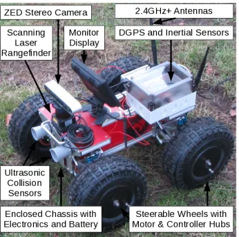
The mobile robot platform used as the rover in this work is designed to meet these challenges, and is shown in Figure 3. Mobility is improved by articulation of the chassis to allow the front and back halves of the rover to rotate and keep all four wheels in contact with the ground. Each of the four wheels contains an integrated DC brush gearhead motor and controller within the wheel hub that is sealed to prevent moisture and dirt ingress. All four wheels are steerable by means of small linear actuators, contain encoders for measuring wheel speed and distance of travel, and can rotate a full 45 degrees in mutual opposition to allow the rover to rotate on the spot if desired. Power is provided by a 22 amp-hour lithium-polymer battery pack, which contains enough power for an 8-hour period of outdoor operation, and it is planned to provide solar recharging stations in the field so that automated recharging without returning to a single location will be possible.

Measurement Unit (IMU) board with a three degree of freedom accelerometer, angular rate sensor, and magnetometer. Communications and telemetry from the rover is provided using an Intel Mini-PCI 2.4GHz Wi-Fi card. Sensing of the surroundings is performed primarily with a Stereolabs ZED stereo vision camera mounted on the front of the rover. Sensing of obstacles in an arc around the rover is provided by a Hokuyo UTM-30LX-EW scanning laser rangefinder. Finally, absolute localization is available by using a U-Blox C94-M8P differential GPS receiver. Two MaxBotix XL-MaxSonar-EZ0 ultrasonic range sensors on the front of the rover provide additional capability to detect potential collisions. The Jetson TK1 and ZED stereo camera cost in the hundreds of Euros and the total cost of the sensing and processing hardware is below a thousand Euros, making this platform affordable to farmers. Only the scanning laser rangefinder is con-sidered a high-priced component with a cost in the thousands of Euros, and may become affordable in the near future due to advancements in solid-state LIDAR technology.

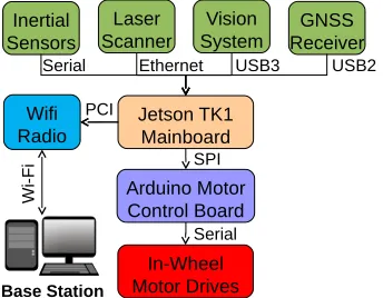
The total weight of the rover platform is 15.5kg. The sensors are small and leave the entire back half area on top of the rover for payloads, which will in future include a laser-induced breakdown spectrometer (LIBS) system for mea-suring chemical components of soil such as Nitrogen, and a lightweight mechan-ical arm with three degrees of freedom for camera-based crop inspection and sample cutting. Figure 4 contains a representation of the hardware components and their connections. Inertial sensors are connected directly via logic-level se-rial to the Jetson TK1, which performs all sensor processing operations. The Hokuyo scanning laser rangefinder is connected via Ethernet, the ZED stereo camera by USB3, and the DGPS unit by USB2. Localization, mapping and mo-tion planning are performed by the Jetson TK1, which then sends direcmo-tional movement commands consisting of desired speed and steering rate are sent at a rate of 100Hz to the Arduino board for kinematic transformation. The required steering angles and motor speeds are communicated to the motor controllers and steering actuators via logic-level serial and pulse-width modulation (PWM).

The software used for sensory processing, localization and mapping, and mo-tion planning on the NVidia Jetson TK1 board is based on the Robot Operating System middleware (ROS Indigo), which runs within an Ubuntu Linux 14.04 operating system environment. This enables a large array of open-source soft-ware modules developed by the ROS community to be used, including many that implement results from other research projects. ROS nodes may be con-nected to sensors or actuators, or they may be intermediate nodes that process data. Sensor-connected nodes broadcast sensor information via topics in the ROS system, so that other nodes may use them as inputs for computation, actuator-connected nodes read information from ROS topics and output commands to their controllers, and other nodes simply process information from topics while broadcasting new topics. Our system contains four ROS sensor nodes: an IMU node (razor imu 9dof), a ZED stereo camera node (zed-ros-wrapper), a laser scanner node (hokuyo node) and a GPS node (nmea navsat driver).

Several intermediate nodes that are available as part of the ROS community perform various navigation processing tasks as follows:

– A transform broadcaster publishes information regarding the relative move-ment of the rover parts.

– A GPS transform node (navsat transform node) converts the GPS coordi-nates to approximate 2-D orthogonal coordicoordi-nates in a fixed Cartesian Coor-dinate System parallel to the rover plane of operation.

– A Hector-SLAM node [Kohlbrecher et al., 2011] converts laser readings into odometry estimation according to the displacement of laser-detected objects. – A visual odometry node converts information from the stereo camera into

es-timation of robot movements, and an extended Kalman Filter node [Moore and Stouch, 2014] fuses all the odometry information and the velocity and orientation

informa-tion from the IMU to produce one final global odometry estimate.

– An RTAB-MAP node [Labb´e and Michaud, 2014] uses the final odometry estimate and the camera data to reconstruct a 3-D and 2-D representation of the environment

– A map-server node manages complex maps by decomposing them into mul-tiple smaller parts and provides these partial maps when needed

Several new ROS nodes were written specifically for the agricultural rover platform to improve performance in outdoor agricultural navigation tasks in the context of farm monitoring as follows:

– A custom-designed controller node sets wheel speed for all four wheels, con-trols the wheel angles through the linear actuators for steering, and feeds back wheel and steering odometry via the SPI interface to the Arduino board. – As most existing path planners are precise in nature and do not perform well in uncertain or changing environments, a path planner node was created with a simplified algorithm for choosing uncomplicated paths efficiently through open spaces such as farm fields.

takes a global plan and sends command to the wheel controller, moreover it stops the rover in the advent of unmapped obstacles such as passing animals, a navigator node store the set of goals that a user may input into the rover and oversees the execution of the plan.

– Finally a connector node connects ROS to an external user interface, such interface is the point of access of a farmer and it offers the ability to look at the re-constructed map and input high level goals to the rover, such as sampling at multiple destinations.

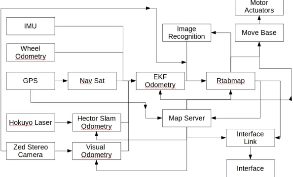
These new ROS nodes perform the key functions that allow the rover to per-form in agricultural environments. Figure 5 shows an overview of the architecture of the software system.

Fig. 5.Software Architecture

3

Sensor Fusion for Odometry

Farming fields pose a significant challenge to robot visual localization due to the uniformity of terrain and external features. Each part of a field or or-chard looks very much the same visually or in terms of solid obstacles, and even when navigating down crop rows, ongoing visual measurement of distances is a challenge. The Hokuyo UTM-30LX-EW laser scanner, which performs very well in an indoor environment with walls and well-defined obstacles, cannot provide consistent tracking in a sparse, unchanging or empty environment. Initially, vi-sual odometry and mapping using the ZED stereo camera and RTAB-Map was evaluated as a single sensory method, producing a good-quality 3D representa-tion of our lab and some outdoor areas in which features are rich in complex, recognizable objects such as the grove of trees shown in Figure 6. However, experimenting with RTAB-MAP under different system configurations made it clear over time that small errors in the odometry estimation caused the 3-D objects to shift in space and produce very bad reconstructions, and in outdoor environments it is generally not possible to reproduce good quality 3-D maps like these in real time.

Fig. 6.High-quality 3-D reconstruction of a grove of trees on a farm from RTAB-Map. Visual odometry is consistent only while differences between locations in the scene are obvious and discernible.

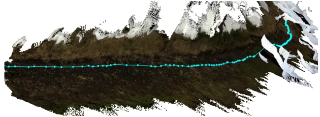
loop closures are subject to optimization once a map has been created. In the agricultural context the greatest challenge is traversal across farmers’ fields, in which case very few nearby visual references are available for odometry and loop closure. Figure 7 shows a navigational map obtained from a farm field with a fenced boundary, in which good visual odometry is maintained as long as distinct objects around the boundary are present. This represents a relatively easy map to obtain at a speed of approximately 0.5 m/s due to the diversity of features available and navigation is straightforward as long as the boundary is in view of the rover. A more difficult situation is shown in Figure 8, where the farm field boundary is grassy and lacking in distinct features. A slower forward speed of 0.2 m/s or lower is necessary to perform mapping while travelling along the boundary of this field, and visual odometry is less consistent. It is still possible to maintain good odometry when travelling along the perimeter of this field as long as some features are tracked well. However, as soon as the boundary is out of the rover’s view when entering the centre of the field, odometry is easily lost and the integrity of the map is compromised.

Fig. 7.High-quality 3-D reconstruction of a farm field with fenced border from RTAB-Map. As long as the border is in view, visual odometry can be maintained.

To evaluate the quality of odometry in a general outdoor environment, a test was run in which five points were chosen in a 100 square meter area and their relative position from a starting point was measured. The rover was man-ually driven through each of the five points, and the odometry estimation was recorded. Table 1 reports the average error from these tests between real position and recorded odometry under different configurations of the extended Kalman Filter node. The left columns indicate the sensor information that has been fused in the EKF node, and the rightmost column contains the average error in meters. The smallest error recorded in this test was 1.77 meters.

This experiment confirms that while the laser scanner is the most reliable sensor indoors, it provides little reliable information in a large outdoor area. The irregular shapes of the plants does not only offer a challenge in tracking for the Hector-Slam node in the reconstruction of a 2-D laser map, but the uneven terrain also causes frequent false obstacles to be detected even when pose is corrected via the IMU. Repeated 3D reconstruction attempts have proved that the error becomes too large to produce a full 3-D map of a farm field. As a result, emphasis in the mapping process is now being shifted to producing a reliable 2-D obstacle map that can be overlaid on a topographic elevation map.

Table 1.The average fused odometry error in localizing at five points in a 100 squared meter outdoor area with respect to the different sensors fused by the EKF node

Laser Odometry Visual Odometry Linear Velocity Visual Odometry Angular Velocity IMU Orientation IMU Angular Velocity IMU Linear Acceleration GPS Wheel Odometry Linear Velocity Wheel Odometry Angular Velocity Error in Meters absolute 6.81

absolute absolute 2.22

absolute absolute 4.01

absolute absolute 4.31

absolute absolute absolute 2.74

absolute absolute 5.13

absolute absolute 2.95

absolute differential 7.14

absolute differential absolute absolute 6.03

absolute absolute 7.92

absolute absolute 5.25

absolute absolute absolute 5.96

absolute absolute 4.61

absolute differential 7.99

absolute differential differential 4.26

absolute absolute absolute absolute 8.10

4

Local Planner

The rover originally made use of the ROS planners available for the move base node, which provides a general infrastructure to integrate different pairs of global and local planners. The node requires a 2-D occupancy map and a set of goal locations to compute a global plan and output velocity commands in real time to the drive motors until the destination is reached. The local plan-ner algorithms tested included the standard base local planplan-ner for differential drive, dwa local planner (dynamic window approach), eband local planner (elas-tic band), and teb local planner (timed elas(elas-tic band). The global planner used in all cases was the basic Navfn global planner in ROS since it provides valid planning around mapped obstacles. However, it was found that these ROS-based planners made critical assumptions about the underlying mobility hardware, in particular that commands and odometry feedback would be executed with neg-ligible time lag and that small incremental movements by pulsing the motors would be possible. As the rover platform uses four-wheel steering and takes time to accelerate and turn, the planning algorithms would repeatedly issue com-mands for small, incremental angular adjustments (or in the case of the ROS teb local planner, back-and-forth steering movements) and when this failed due to either actuator lag or lack of precise movement, execute recovery behaviours. To remedy this problem, we developed a new and simplified planner that relaxed the constraints on timing and precision in favour of a best-effort approach.

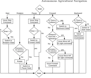
For trial testing, we created a very simple algorithm: at the start the rover rotates on the spot and aligns itself along the direction of the global path, then it tries to follow the path by steering when needed either when the direction of the curves changes too much or the rover moves too far away from the plan. Once the destination is reached a signal is sent to the navigator nodes which may provide another goal or halt the rover. The planner uses five states of operation with appropriate commands sent to the drive motors for the duration of each state: Start, Forward, Backward, Pause, and Rotation. A flowchart of the process the planner uses when moving from the current movement state to the next movement state is given in Figure 11.

Making use of high-quality odometry information that is available by using Hector SLAM and the scanning laser rangefinder in the lab environment, this planner showed much better reliability than the ROS planners on the rover platform. In trial runs for this planner, seven different points were set spaced far apart on the lab floor and the rover was directed to visit them autonomously in order. Table 5 reports the distance between the set goals and the point the rover stopped at, and an average error of 15cm was recorded at the points the rover stopped. Figure 12 shows the 2-D Hector SLAM and reconstructed 3-D RTAB-Map maps of our lab and the testing path: S marks the starting point and each numbered goal point is marked G. The goals are structured in order of the difficulty of reachability:

1. from S to G1 there is a straight path

Fig. 9.Flowchart of the navigational planner process. The planner sends commands to the drive motors while in each of five states, and state transitions are performed where indicated.

3. from G3 to G4 there is a sharp corner 4. from G5 to G6 there is a narrow path

5. from G6 to G7 the path includes a narrow door

The same experiment was executed in an outdoor area. Unfortunately, due to the low mapping quality and the higher position uncertainty of the rover in outdoor environment, the rover could reach only the first goal with an error of 1-2 meters and was not able to reach the following ones. Table 6 reports the distance between the set goal and the point the rover stopped at.

The above experiments for evaluating the quality of odometry make use of manual measurements of the reference position of the robot. All odometry mea-sures indirectly computed from the sensors and the sensor fusion are compared to this reference to compute the error. However, manual measurements are sub-ject to error due to difficulty of making the robot pass exactly though the chosen locations. We also observed that Hector-Slam scanning laser based localization is very precise when there are enough distinct laser-detectable features surround-ing of the robot. In such a scenario, the localization error is approximated by the laser resolution, and is comparable to our manual measurement error. Hence, we devised a more data-dense experiment that uses as a reference the odometry computed by Hector Slam localization.

Table 2.The navigation error in the lab environment for each one of the six goals, depending on the enabled sensors (NR stands for Not Reached)

Laser Odometry

Other Sensors

Measure Goal 1 Error (cm)

Goal 2 Error (cm)

Goal 3 Error (cm)

Goal 4 Error (cm)

Goal 5 Error (cm)

Goal 6 Error (cm)

Goal 7 Error (cm)

absolute 0 20 20 NR NR NR NR

absolute IMU Angular Velocity 0 5 15 0 0 0 NR absolute IMU Linear Acceleration 25 10 35 NR NR NR NR absolute IMU Both above measures 0 20 35 0 20 NR NR absolute Visual Odom. Linear Velocity 20 30 5 5 NR NR NR absolute Visual Odom. Angular Velocity 0 10 25 0 0 20 NR absolute Visual Odom. All Velocities 0 50 20 5 40 20 NR absolute Wheel Odom. Linear Velocity 70 30 30 0 NR NR NR absolute Wheel Odom. Angular Velocity 10 60 25 150 25 0 NR absolute Wheel Odom. All velocities 5 NR NR NR NR NR NR

Table 3.The navigation error in garden environment for one goal located 15 meters ahead of the starting position, depending on the enabled sensors. NR stands for Not Reached.

Laser Odometry

Other Sensors

Measure Goal

Error in meters

absolute 1.5

absolute IMU Angular Velocity 2

absolute IMU Linear Acceleration 3 absolute Visual Odom. Linear Velocity 0.5 absolute Visual Odom. Angular Velocity NR absolute Wheel Odom. Linear Velocity 1 absolute Wheel Odom. Angular Velocity 1.5

error due to feature matching uncertainty. While moving, the robot computes its reference pose using Hector-Slam and the odometry evaluation using different sensors with different combinations of sensor fusion. As soon as the odometry information is available, they are compared to the current Hector-Slam pose and the distance error and angle error are stored for analysis. This experiment allows us to quickly gather a larger quantity of data and compute the average odometry error.

Table 7 shows the distance errors and the angle errors for each combination of fused sensors. The errors depend on the different sensors fused by the EKF node and have been computed as follows:

The average relative distance error (meters) is

eARD= n

X

i=0

||odometry posei−laser posei||

Pi

t=1||laser poset−laser poset−1||

. (1)

The average angular error (radians) is

eAAD= n

X

i=0

min(odometry orientationi−laser orientationi)

n (2)

where

min(α, β) =asb(α−β)−(2∗k+ 1)∗π (3) and kis the integer part of asb₂(α_∗π−β). The final relative distance error (meters) is:

eF RD=

||odometry posen−laser posen||

Pi

t=1||laser poset−laser poset−1||

. (4)

The final angular error (radians) is

Table 4. The average fused odometry error on a 55 metre path with a cumulative turning angle of 190 radians.

Visual Odometry

IMU Wheel

Odometry

eARD eF RD eAADeF AD

Planar Coordinates Orientation

6.45% 2.64% 1.45 0.59

Planar Coordinates Orientation

2.60% 2.04% 0.20 0.94

Planar Coordinates Orientation Linear Velocity Angular Velocity Linear Velocity Angular Velocity

18.99% 6.02% 1.72 1.16

Differential Orientation Angular Velocity Linear Acceleration Planar Coordinates Orientation Linear Velocity Angular Velocity

7.42% 1.76% 1.09 0.37

Planar Coordinates Orientation Linear Velocity Angular Velocity Differential Orientation Angular Velocity Linear Acceleration

8.30% 2.04% 1.09 0.33

Planar Coordinates Orientation Linear Velocity Angular Velocity Differential Orientation Angular Velocity Linear Acceleration Linear Velocity Angular Velocity

6.40% 5.98% 1.09 0.34

Linear Velocity Angular Velocity Planar Coordinates Orientation Linear Velocity Angular Velocity

18.36% 6.72% 1.71 1.68

Linear Velocity Angular Velocity Differential Orientation Angular Velocity Linear Acceleration Planar Coordinates Orientation Linear Velocity Angular Velocity

6.50% 6.02% 1.09 0.34

Planar Coordinates Linear Velocity Angular Velocity

Orientation Linear Velocity Angular Velocity

5.40% 7.36% 1.09 0.29

Orientation Angular Velocity Linear Acceleration Planar Coordinates Linear Velocity Angular Velocity

4.68% 1.71% 1.09 0.29

Planar Coordinates Linear Velocity Angular Velocity Orientation Angular Velocity Linear Acceleration

5.82% 1.85% 1.09 0.29

Planar Coordinates Linear Velocity Angular Velocity Orientation Angular Velocity Linear Acceleration Linear Velocity Angular Velocity

4.56% 5.64% 1.09 0.29

Linear Velocity Angular Velocity

Orientation Planar Coordinates Linear Velocity Angular Velocity

5.34% 7.36% 1.09 0.29

Linear Velocity Angular Velocity Orientation Angular Velocity Linear Acceleration Planar Coordinates Linear Velocity Angular Velocity

5

Local Planner

The rover originally made use of the ROS planners available for the move base node, which provides a general infrastructure to integrate different pairs of global and local planners. The node requires a 2-D occupancy map and a set of goal locations to compute a global plan and output velocity commands in real time to the drive motors until the destination is reached. The local plan-ner algorithms tested included the standard base local planplan-ner for differential drive, dwa local planner (dynamic window approach), eband local planner (elas-tic band), and teb local planner (timed elas(elas-tic band). The global planner used in all cases was the basic Navfn global planner in ROS since it provides valid planning around mapped obstacles. However, it was found that these ROS-based planners made critical assumptions about the underlying mobility hardware, in particular that commands and odometry feedback would be executed with neg-ligible time lag and that small incremental movements by pulsing the motors would be possible. As the rover platform uses four-wheel steering and takes time to accelerate and turn, the planning algorithms would repeatedly issue com-mands for small, incremental angular adjustments (or in the case of the ROS teb local planner, back-and-forth steering movements) and when this failed due to either actuator lag or lack of precise movement, execute recovery behaviours. To remedy this problem, we developed a new and simplified planner that relaxed the constraints on timing and precision in favour of a best-effort approach.

For trial testing, we created a very simple algorithm: at the start the rover rotates on the spot and aligns itself along the direction of the global path, then it tries to follow the path by steering when needed either when the direction of the curves changes too much or the rover moves too far away from the plan. Once the destination is reached a signal is sent to the navigator nodes which may provide another goal or halt the rover. The planner uses five states of operation with appropriate commands sent to the drive motors for the duration of each state: Start, Forward, Backward, Pause, and Rotation. A flowchart of the process the planner uses when moving from the current movement state to the next movement state is given in Figure 11.

Making use of high-quality odometry information that is available by using Hector SLAM and the scanning laser rangefinder in the lab environment, this planner showed much better reliability than the ROS planners on the rover platform. In trial runs for this planner, seven different points were set spaced far apart on the lab floor and the rover was directed to visit them autonomously in order. Table 5 reports the distance between the set goals and the point the rover stopped at, and an average error of 15cm was recorded at the points the rover stopped. Figure 12 shows the 2-D Hector SLAM and reconstructed 3-D RTAB-Map maps of our lab and the testing path: S marks the starting point and each numbered goal point is marked G. The goals are structured in order of the difficulty of reachability:

1. from S to G1 there is a straight path

3. from G3 to G4 there is a sharp corner 4. from G5 to G6 there is a narrow path

5. from G6 to G7 the path includes a narrow door

The same experiment was executed in an outdoor area. Unfortunately, due to the low mapping quality and the higher position uncertainty of the rover in outdoor environment, the rover could reach only the first goal with an error of 1-2 meters and was not able to reach the following ones. Table 6 reports the distance between the set goal and the point the rover stopped at.

Table 5.The navigation error in the lab environment for each one of the six goals, depending on the enabled sensors (NR stands for Not Reached)

Laser Odometry

Other Sensors

Measure Goal 1 Error (cm) Goal 2 Error (cm) Goal 3 Error (cm) Goal 4 Error (cm) Goal 5 Error (cm) Goal 6 Error (cm) Goal 7 Error (cm)

absolute 0 20 20 NR NR NR NR

absolute IMU Angular Velocity 0 5 15 0 0 0 NR absolute IMU Linear Acceleration 25 10 35 NR NR NR NR absolute IMU Both above measures 0 20 35 0 20 NR NR absolute Visual Odom. Linear Velocity 20 30 5 5 NR NR NR absolute Visual Odom. Angular Velocity 0 10 25 0 0 20 NR absolute Visual Odom. All Velocities 0 50 20 5 40 20 NR absolute Wheel Odom. Linear Velocity 70 30 30 0 NR NR NR absolute Wheel Odom. Angular Velocity 10 60 25 150 25 0 NR absolute Wheel Odom. All velocities 5 NR NR NR NR NR NR

Table 6.The navigation error in garden environment for one goal located 15 meters ahead of the starting position, depending on the enabled sensors. NR stands for Not Reached. Laser Odometry Other Sensors Measure Goal Error in meters absolute 1.5

absolute IMU Angular Velocity 2

absolute IMU Linear Acceleration 3 absolute Visual Odom. Linear Velocity 0.5 absolute Visual Odom. Angular Velocity NR absolute Wheel Odom. Linear Velocity 1 absolute Wheel Odom. Angular Velocity 1.5

6

GPS-only navigation

restrictive scenario. We assumed that the rover had to move autonomously in an open empty field devoid of insurmountable obstacles. The field is allowed to contain cliffs, hills and rocks as long as the rover is able to climb upon them. The rationale of the scenario is that a farmer may need to collect soil samples in a grassy or recently plowed field. Moreover, the roughness of the terrain may cause a lot of stress on the wheels actuators when the rover is trying to perform a turn on the spot. Hence we disable this feature in the new navigation system and we require that the rover turns by steering.

The new navigation system relies on two sensors: a differential GPS and a compass integrated into an IMU unit. The differential GPS measure is obtained by connecting two GPS units by a radio link. One GPS unity is located on the rover and the other is mounted on a fixed isolated mast and provides correcting measures. The compass provides the 3d angle toward the north direction. The GPS coordinates are transformed in a local 2D Cartesian coordinates system with center on the starting position of the rover and y axis given by the north direction. The 3d heading angle is transformed into its planar projection on the base plane of the rover, and we use this projection as an approximation of the heading angle in the 2d coordinate system.

The position of a target destination is given as GPS coordinates and is pro-jected on the local 2D Cartesian system. A global planner computes the shortest path composed by a circular line and a straight line from the current position (coordinates and heading) to the destination. The circular line may appear be-fore or after the straight line and it is required in order to adjust the heading direction in such a way that the rover points toward the target.

A local planner ensures that the rover follows the circular line and the straight line, and asks for a re-computation of the global plan if the rover moves acci-dentally too far away. The main challenge encountered during the design of the local planner has been the measurement error of the compass. Small errors in the compass reading ( 5-10 degrees) cause the rover to move away from the target path and a constant re-adjustment is needed. A measure of the distance between the target line and the rover is computed along the different between the rover heading and the ideal heading it should have along the target line. If the rover is trying to follow a circular line, then a new circle is computed with the aim of converging to the target circle, and the velocity commands necessary to follow the new circles are sent to the motor controllers. If the rover is trying to move along a straight line then the correction is applied according to angle and distance with fixed values according to some thresholds.

Under the scenario assumption, as long as the human operator provides target goals with a free direct path to the rover position, the rover is safe to move along the line.

into the ground, analyze the sample and record the data. A remote visualization tool allowed us to read the measure as it was extracted. The rover managed to reach 12 points with the same distance error provided by the GPS system., before the it had mechanical problems and repairs were needed. During the test, the navigation system was not optimal. The rover tended to diverge from the planned path, a few times the target was missed and a new plan was recomputed. Since the rover had to turn back along a circle, missing a target considerably increased the navigation time. Figure 14 shows a successful navigation where the rover did not need to re-plan the target path.

Fig. 13.Farm field in the Glasgow country area. 24 points were selected as destination targets. Red line shows the path in the farming field.

We also tested the navigation system in an open spot in the garden of the university. In this place, the navigation system did not work at all, because the compass reading were consistently wrong at given locations. We hypothesize that the presence of magnetic interference, may cause the compass to provide false measures in a city center.

Fig. 14.Planned path compared to actual path on a 2D local map representation.

the Kalman filter was not able to eliminate all the errors because also the GPS had an increased error measure. Moreover, in the open empty field, we analyzed the estimated 2d local positions with and without a Kalman filter during a rover test, and we observed that the two measures had comparable errors.

7

Greenhouse

We also focused on a second more restrictive scenario. We assumed that the rover had to harvest fruits in a greenhouse environment. Hence, it had to move in small areas surrounded by unsurmountable obstacles. The terrain is mostly flat and the rover does not need to climb obstacles and experience changes of inclination.

The navigation system relies on three sensors: a 2d laser scanner for the detection of obstacles in a 270 degree window on the plane of the rover, an IMU for the detection of the rover inclination, and a set of sonar mounted at the back for the detection of the obstacle in the visual window which is not covered by the laser.

inclination (for example on a very rough terrain), Hector Slam may produce an incorrect map. For example, when the rover bends forward, the laser scanner may hit the ground, and an obstacle may be detected in the front and it may be placed in the map. The error may produce an incorrect localization and cause the construction of a wrong map. We often witnessed the problem during the setting of the working parameters of Hector Slam. Falling with only on wheel in a small hole in the ground, or climbing a steep obstacle caused a complete loss of localization.

Since the rover needs to move in a constrained environment, we cannot allow it to move along large steering circle like it happened in the open field scenario. Orientation toward the correct heading direction is achieved by using backward steering manoeuvres alternated with forward steering manoeuvres. Hence, we implement backward obstacle detection as well. The sonar sensors are used for this purpose, however they easily fail to detect obstacles or are too slow to re-spond. Hence, the main obstacle detection function is entrust to the map produce by Hector Slam. The localized rover position is compared with the position of the obstacle to detect current or future collisions and halt the rover accordingly. Hence, as long as the obstacles in the back of the rover are mapped the rover safely halts during a backward manoeuvre. If the rover starting position has no obstacles immediately in the back or the first destination is set immediately in front of the rover, backward manoeuvres do not cause collisions.

The global planner computes a path from the starting position to the target position by heuristic depth search in a partial pose tree. The pose tree has root given by the rover starting position, each node of the tree is expanded by adding some neighbour poses at a given distance along a fixed set of directions. The neighbours are added as long as they do not cross an obstacle and do not cause a loop. A priority is assigned to the point according to its distance to the obstacle, whether there is a change of direction and the distance from obstacles(straight lines are preferred, and paths farther away from obstacles are preferred). Positions are explored and expanded as needed. The algorithm stops when a direct path from a pose to the goal is found or a timer runs out. If a path is generate, it is simplified by leaving out only points that are reachable one from the other by a direct line. A new global planner was created due to the following reasons: Ros global planner would fail to compute a plan if the rover moves too close to an obstacle by accident. On the converse, if the obstacle tolerance is increased, the planner would compute a path very close to the obstacles which would make the navigation hazardous.

Table 7. The average fused odometry error on a 55 metre path with a cumulative turning angle of 190 radians.

Visual Odometry

IMU Wheel

Odometry

eARD eF RD eAADeF AD

Planar Coordinates Orientation

6.45% 2.64% 1.45 0.59

Planar Coordinates Orientation

2.60% 2.04% 0.20 0.94

Planar Coordinates Orientation Linear Velocity Angular Velocity Linear Velocity Angular Velocity

18.99% 6.02% 1.72 1.16

Differential Orientation Angular Velocity Linear Acceleration Planar Coordinates Orientation Linear Velocity Angular Velocity

7.42% 1.76% 1.09 0.37

Planar Coordinates Orientation Linear Velocity Angular Velocity Differential Orientation Angular Velocity Linear Acceleration

8.30% 2.04% 1.09 0.33

Planar Coordinates Orientation Linear Velocity Angular Velocity Differential Orientation Angular Velocity Linear Acceleration Linear Velocity Angular Velocity

6.40% 5.98% 1.09 0.34

Linear Velocity Angular Velocity Planar Coordinates Orientation Linear Velocity Angular Velocity

18.36% 6.72% 1.71 1.68

Linear Velocity Angular Velocity Differential Orientation Angular Velocity Linear Acceleration Planar Coordinates Orientation Linear Velocity Angular Velocity

6.50% 6.02% 1.09 0.34

Planar Coordinates Linear Velocity Angular Velocity

Orientation Linear Velocity Angular Velocity

5.40% 7.36% 1.09 0.29

Orientation Angular Velocity Linear Acceleration Planar Coordinates Linear Velocity Angular Velocity

4.68% 1.71% 1.09 0.29

Planar Coordinates Linear Velocity Angular Velocity Orientation Angular Velocity Linear Acceleration

5.82% 1.85% 1.09 0.29

Planar Coordinates Linear Velocity Angular Velocity Orientation Angular Velocity Linear Acceleration Linear Velocity Angular Velocity

4.56% 5.64% 1.09 0.29

Linear Velocity Angular Velocity

Orientation Planar Coordinates Linear Velocity Angular Velocity

5.34% 7.36% 1.09 0.29

Linear Velocity Angular Velocity Orientation Angular Velocity Linear Acceleration Planar Coordinates Linear Velocity Angular Velocity

The above experiments for evaluating the quality of odometry make use of manual measurements of the reference position of the robot. All odometry mea-sures indirectly computed from the sensors and the sensor fusion are compared to this reference to compute the error. However, manual measurements are sub-ject to error due to difficulty of making the robot pass exactly though the chosen locations. We also observed that Hector-Slam scanning laser based localization is very precise when there are enough distinct laser-detectable features surround-ing of the robot. In such a scenario, the localization error is approximated by the laser resolution, and is comparable to our manual measurement error. Hence, we devised a more data-dense experiment that uses as a reference the odometry computed by Hector Slam localization.

In this experiment, we manually drove the robot in our lab, which is rich in asymmetric planar features and allows Hector Slam to minimize the localization error due to feature matching uncertainty. While moving, the robot computes its reference pose using Hector-Slam and the odometry evaluation using different sensors with different combinations of sensor fusion. As soon as the odometry information is available, they are compared to the current Hector-Slam pose and the distance error and angle error are stored for analysis. This experiment allows us to quickly gather a larger quantity of data and compute the average odometry error.

Table 7 shows the distance errors and the angle errors for each combination of fused sensor. The errors depend on the different sensors fused by the EKF node.

The errors have been computed as follows: The average relative distance error (meter) is

eARD= n

X

i=0

||odometry posei−laser posei||

Pi

t=1||laser poset−laser poset−1||

. (6)

The average angular error (radians) is

eAAD= n

X

i=0

min(odometry orientationi−laser orientationi)

n (7)

where

min(α, β) =asb(α−β)−(2∗k+ 1)∗π (8) andkis the integer part of asb₂(α_∗π−β). The final relative distance error (meter) is:

eF RD=

||odometry posen−laser posen||

Pi

t=1||laser poset−laser poset−1||

. (9)

The final angular error (radians) is

8

Conclusion

In this chapter we have introduced a light weight and low cost agricultural robot platform for autonomous environment monitoring, and discussed autonomous guidance and planning technologies implemented in ROS for odometry and lo-calization, identification of objects, and path planning under limited kinematic precision. Our results to date regarding navigation indicate that this agricul-tural vehicle can successfully reach set navigational points with high precision so long as accurate and real-time localization is available such as that provided by Hector SLAM against fixed obstacles. We have also proved that the meth-ods used for indoor and feature-rich localization and odometry are not suitable for use outdoors in uniformly-visual farm fields. We are nonetheless able using a low-cost robot platform with a minimal sensor set to traverse navigational goals efficiently and quickly using a simple, efficient, and kinematically-tolerant planning algorithm for our robot platform.

The next steps in our ongoing work to develop this platform include the in-tegration of differential GNSS localization between a local base station and the robot using the recently-released u-blox C94M8P DGPS devices to be a supple-ment for odometry in feature-poor field environsupple-ments, and the integration of soil sampling and visual measurement technologies to allow autonomous monitoring activities to be tested in the field. In future, machine vision based navigation will be able to tolerate harsher weather conditions. An intelligent path planning algorithm using probabilistic mapping and optimization methods will be used for more challenging farming operations.

ACKNOWLEDGEMENTS

References

[Bechar and Vigneault, 2016] Bechar, A. and Vigneault, C. (2016). Agricultural robots for field operations: concepts and components. Biosystems Engineering, 149:94–111. [Bengochea-Guevara et al., 2016] Bengochea-Guevara, J. M., Conesa-Munoz, J., An-dujar, D., and Ribeiro, A. (2016). Merge fuzzy visual servoing and gps based planning to obtain a proper navigation behavior for a small corp inspection robot. Sensors, 16(3).

[Blackmore et al., ] Blackmore, B. S., Griepentrog, H. W., Nielsen, H., and Norremark, M. Development of a deterministic autonomous tractor. Inthe CIGR International Conference, Beijing, China, November 2004.

[Bochtis et al., 2010] Bochtis, D. D., Sorensen, C. G., and Vougioukas, S. G. (2010). Path planning for in field nagivation aiding of service units. Computers and Elec-tronics in Agriculture, 74(1):80–90.

[Cho and Lee, 2000] Cho, S. I. and Lee, J. H. (2000). Autonomous speedsprayer using differential global positioning system, genetic algorithm and fuzzy control. Journal of Agricultural Engineering Research, 76(2):111–119.

[Emmi et al., 2014] Emmi, L., Gonzalez de Soto, M., Pajares, G., and de Santos, G. (2014). New trends in robotics for agriculture: integration and assessment of a real fleet of robots. The Scientific World Journal, 21:1–22.

[Grimstad and From, 2017] Grimstad, L. and From, P. J. (2017). The thorvald ii agri-cultural robotic system. Robotics MDPI, 6(24):1–17.

[Hague et al., 2000] Hague, T., Marchant, J. A., and Tillett, N. D. (2000). Ground based sensing systems for autonomous agricultural vehicles. Cumputers and Elec-tronics in Agriculture, 25(1-2):11–28.

[Hajjaj and Sahari, 2017] Hajjaj, S. S. H. and Sahari, K. S. M. (2017). Bringing ros to agriculture automation: hardware abstraction of agriculture machinery.International Journal of Applied Engineering Research, 12(3):311–316.

[Hameed, 2014] Hameed, I. A. (2014). Intelligent coverage path planning for agri-cultural robots and autonomous machines on three dimensional terrain. Joural of Intelligent and Robotic Systems, 74(3-4):965–983.

[Hameed et al., 2016] Hameed, I. A., La Cour-Harbo, A., and Osen, O. L. (2016). Side to side 3d coverage path planning approach for agricultural robots to minimize skip/overlap areas between swaths. Robotics and Autonomous Systems, 76:36–45. [Hayashi et al., 2010] Hayashi, S., Shigematsu, K., Yamamoto, S., Kobayashi, K.,

Kohno, Y., Kamata, J., and Kurita, M. (2010). Evaluation of a strawberry-harvesting robot in a field test. Biosyst. Eng., 105:160–171.

[Hayashi et al., 2012] Hayashi, S., Yamamoto, S., Saito, S., Ochiai, Y., Kohno, Y., Yamamoto, K., Kamata, J., and Kurita, M. (2012). Development of a movable strawberry-harvesting robot using a travelling platform. In Proc. Int. Conf. Agric. Eng. CIGR-AgEng 2012, Valencia, Spain.

[Henten et al., 2003a] Henten, E. V., Tuijl, B. V., Hemming, J., Kornet, J., and Bontsema, J. (2003a). Collision-free motion planning for a cucumber picking robot. Biosyst. Eng., 86:135–144.

[Henten et al., 2003b] Henten, E. V., Tuijl, B. V., Hemming, J., Kornet, J., Bontsema, J., and van Os, E. A. (2003b). Field test of an autonomous cucumber picking robot. Biosyst. Eng., 86:305–313.

[Jensen et al., 2014] Jensen, K., Larsen, M., Nielsen, S. H., Larsen, L. B., Olsen, K. S., and N, J. R. (2014). Towards an open software platform for field robots in precision agriculture. Robotics, 13:207–234.

[Jiang et al., 2014] Jiang, D. w., Yang, L. C., Li, D. H., Gao, F., Tian, L., and Li, L. J. (2014). Development of a 3d ego motion estimatioon system for an autonoumous agricultural vehicle. Biosystems Engineering, 121:150–159.

[Katupitiya et al., 2007] Katupitiya, J., Eaton, R., and Yaqub, T. (2007). Systems engineering approach to agricultural automation: New developments. In1st Annual IEEE Syst. Conf., pages 298–304.

[King, 2017] King, A. (2017). Technology: The future of agriculture. Nature, 544:21– 23.

[Kohlbrecher et al., 2011] Kohlbrecher, S., Meyer, J., von Stryk, O., and Klingauf, U. (2011). A flexible and scalable slam system with full 3d motion estimation. InProc. IEEE International Symposium on Safety, Security and Rescue Robotics (SSRR). IEEE.

[Krahwinkler et al., 2011] Krahwinkler, P., Roßmann, J., and Sondermann, B. (2011). Support vector machine based decision tree for very high resolution multispectral forest mapping. In2011 IEEE International Geoscience and Remote Sensing Sym-posium, IGARSS 2011, Vancouver, BC, Canada, July 24-29, 2011, pages 43–46. [Labb´e and Michaud, 2014] Labb´e, M. and Michaud, F. (2014). Online global loop

clo-sure detection for large-scale multi-session graph-based SLAM. In 2014 IEEE/RSJ International Conference on Intelligent Robots and Systems, Chicago, IL, USA, September 14-18, 2014, pages 2661–2666.

[Lopes et al., 2016] Lopes, C. M., Graa, J., Sastre, J., Reyes, M., Guzmn, R., Braga, R., Monteiro, A., and Pinto, P. A. (2016). Vineyard yeld estimation by vinbot robot - preliminary results with the white variety viosinho. In11th Int. Terroir Congress. Jones, G. and Doran, N.(eds.), Southern Oregon University, Ashland, USA, pages 458–463.

[Moore and Stouch, 2014] Moore, T. and Stouch, D. (2014). A generalized extended kalman filter implementation for the robot operating system. In Proceedings of the 13th International Conference on Intelligent Autonomous Systems (IAS-13). Springer.

[Perez et al., 2016] Perez, L., Rodrguez, ., Rodrguez, N., Usamentiaga, R., and Garca, D. F. (2016). Robot guidance using machine vision techniques in industrial environ-ments: a comparative review. Sensors, 16(3):1–26.

[Post et al., 2017] Post, M., Bianco, A., and Yan, X. T. (2017). Autonomous navigation with ros for a mobile robot in agricultural fields. In 14th International Conference on Informatics in Control, Madrid, Spain, pages 1–10.

[Post et al., 2016] Post, M. A., Li, J. q., and Quine, B. M. (2016). Planetary micro-rover operations on mars using a bayesian framework for inference and control. Acta Astronautica, 120:295–314.

[Roßmann et al., 2010] Roßmann, J., Jung, T. J., and Rast, M. (2010). Developing virtual testbeds for mobile robotic applications in the woods and on the moon. In 2010 IEEE/RSJ International Conference on Intelligent Robots and Systems, October 18-22, 2010, Taipei, Taiwan, pages 4952–4957.

[Subramanian et al., 2006] Subramanian, V., Burks, T. F., and Arroyo, A. A. (2006). Development of machine vision and laser radar based autonomous vehicle guid-ance systems for citrus grove navigation. Computers and Electronics in Agriculture, 53(2):130–143.

[van Henten et al., 2002] van Henten, E. J., Hemming, J., van Tuijl, B. A. J., Kornet, J. G., Meuleman, J., Bontsema, J., and van Os, E. A. (2002). An autonomous robot for harvesting cucumbers in greenhouses. Auton. Robots, 13(3):241–258.

[Xue et al., 2012] Xue, J., Zhang, L., and Grift, T. E. (2012). Variable field of view ma-chine vision based row guidance of an agricultural robot. Computers and Electronics in Agriculture, 84:85–91.