Nematic liquid crystals doped with nanoparticles : phase behavior and dielectric properties

Chapter 1

Nematic liquid crystals doped with nanoparticles:

phase behavior and dielectric properties

Mikhail A. Osipov∗1and Maxim V. Gorkunov2 1_{Department of Mathematics, University of Strathclyde,}

Glasgow G1 1XH, UK

2_{Shubnikov Institute of Crystallography of the}

Russian Academy of Sciences, 119333 Moscow, Russia Thermodynamics and dielectric properties of nematic liquid crystals doped with various nanoparticles have been studied in the framework of a molecular mean-field theory. It is shown that spherically isotropic nanoparticles effectively dilute the liquid crystal material and cause a de-crease of the nematic-isotropic transition temperature, while anisotropic nanoparticles are aligned by the nematic host and, in turn, may sig-nificantly improve the liquid crystal alignment. In the case of strong interaction between spherical nanoparticles and mesogenic molecules, the nanocomposite possesses a number of unexpected properties: The nematic-isotropic co-existence region appears to be very broad, and the system either undergoes a direct transition from the isotropic phase into the phase-separated state, or undergoes first a transition into the ho-mogeneous nematic phase and then phase-separates at a lower tempera-ture. The phase separation does not occur for sufficiently low nanopar-ticle concentrations, and, in certain cases, the separation takes place only within a finite region of the nanoparticle concentration. For ne-matics doped with strongly polar nanoparticles, the theory predicts the nanoparticle aggregation in linear chains that make a substantial contri-bution to the static dielectric anisotropy and optical birefringence of the nematic composite. The theory clarifies the microscopic origin of im-portant phenomena observed in nematic composites including a shift of the isotropic-nematic phase transition and improvement of the nematic order; a considerable softening of the first order nematic-isotropic tran-sition; a complex phase-separation behavior; and a significant increase of the dielectric anisotropy and the birefringence.

∗_{e-mail: m.osipov@strath.ac.uk}

2 M.A. Osipov and M.V. Gorkunov

1. Introduction

Liquid crystal nanocomposites are considered to be extremely promising materials in which the properties of a liquid crystal (LC), used, for ex-ample, in display applications, are modified/improved by the presence of various nanoparticles (NPs). There are many reports showing that doping of a nematic LC with even a small amount of NPs affects nearly all impor-tant properties of nematic materials, resulting in a decrease of threshold and switching voltages and reducing the switching times of LC displays (see, for example, Refs. 1–5). Suspensions of metal, dielectric and semi-conductor NPs in various nematic LCs have been investigated by many authors and, in particular, doping of nematics with ferroelectric NPs is known to enhance dielectric and optical anisotropy, increase the electro-optic response6,7and improve the photorefractive properties.8 Suspensions of para- and ferromagnetic particles in nematics are promising candidates for magnetically tunable structures, and doping of ferroelectric LCs with metal and silica nanoparticles enables one to improve the spontaneous po-larization and dielectric permittivity and to decrease switching times.9–11 Metal NPs have been also used to widen the temperature range of LC blue phases,12 _{which are important for applications, and enhance random} lasing in the dye-doped LC medium.13 Finally, distributing semiconductor quantum dots in smectic LC-polymers enables one to achieve the positional ordering of nanosize particles.14,15

At the same time, LC-NP composites are also considered as the building blocks of novel metamaterials. Metamaterials, i.e., arrays of sub-wavelength metallic/semiconductor particles, offer a new degree of freedom in control-ling light: they enable tailoring the optical response, achieving very high, very low and negative values of refractive index, permittivity and/or per-meability.16 _{Combining emerging optical metamaterials with LCs provides} a new important quality – tunability, which is of key importance for emerg-ing applications includemerg-ing tunable photonic materials, optically addressed spatial light modulators and dynamic holography. Upon immersing a meta-material into a nematic LC one can switch the LC alignment by external voltages and modify the overall optical properties of the composite.17 _For instance, the localized plasmon resonance of gold NPs can be tuned by changing the refractive index and, in particular, the birefringence of the surrounding LC medium.18–20

ther-modynamic stability of the LC phase. Recently it has been shown10,11 that the dipolar induction interaction between ferroelectric NPs and the surrounding nematic LC medium may result in a substantial decrease of the nematic-isotropic (N-I) transition temperature. It has also been shown experimentally that the N-I transition temperature can be significantly af-fected by the presence of other types of NPs. For example, a decrease of the N-I transition temperature is observed in nematics doped with ap-proximately isotropic silver,21_gold22_{or aerosil particles,}23,24_{while the N-I} transition temperature increases if the nematic LC is doped with strongly anisotropic NPs including nanotubes,25 magnetic nanorods26 and ferro-electric particles.9,10 _{Recently a detailed mean-field molecular theory of} nematic LCs doped with both isotropic and anisotropic NPs has been de-veloped.27 _{The effect of isotropic NPs has also been considered in Ref. 28,} while the effect of the external electric field on the nematic nano-composites has been studied in Ref. 29.

4 M.A. Osipov and M.V. Gorkunov

nano-composites has recently been developed by the authors.33

Strong interaction between NPs may also lead to their aggregation in-cluding the formation of chains of NPs when the interaction is strongly anisotropic. Aggregates of NPs in general, and polar chains in particular, are expected to modify all major properties of nematic nano-composites, including their dielectric and optical properties. Nematic LCs with polar chains should also be very sensitive to external electric fields which may be used for alignment and switching at very low applied voltage.

It has been shown experimentally (see, for example, Refs. 9,34) that the dielectric anisotropy of nematic LCs doped with strongly polar (ferroelec-tric) NPs is dramatically increased. Indeed, a very small molar fraction of ferroelectric NPs (of the order of 10−3) accounts for a contribution of the order of 5−6 to the anisotropy of the dielectric constant, which is compara-ble with the anisotropy of the nematic host. Preliminary estimates indicate that the increase is too strong to be explained without taking into account possible aggregation of NPs and formation of polar chains. There exists some experimental evidence that quantum dots may also form long chains in nematic LCs35 _{even though such NPs are nonpolar.}

Aggregation of NPs in the nematic phase may occur if the inter-particle interaction potential is not strong enough to induce demixing but is still much stronger than the interaction between mesogenic molecules. Strongly anisotropic interaction between NPs, including in particular dipole-dipole one, will lead to the formation of polar chains. It has been shown36 _that the equilibrium chain length strongly depends on the contact interaction potential normalized by the temperature. Long chains of NPs may occur only if the contact interaction is of the order of 10kBT36 which is satisfied,

for example, for ferroelectric NPs.9,34 _{Polar chains should make a significant} contribution to the dielectric anisotropy of nematic composites.

2. Effect of nano-particles on the nematic-isotropic phase transition

2.1. Mean-filed theory of nematic composites

Consider a composite material formed by Nm highly anisotropic identical

LC molecules and Np NPs with possible deviations in physical properties

or shape, size and surface structure. To take into account this NP diversity we assume that there areLdifferent types of NPs in the composite and the number of the NPs of the typel isNl such thatN1+N2+...NL=Np.

Now let Vmol be the part of the total volume V occupied by the LC molecules, while the volume Vp = V −Vmol is occupied by NPs. Then φ = Vp/V is the volume fraction of NPs and the number density of NPs ρp = φ/vp, where vp is the average particle volume. Assuming that the

number density of LC molecules in the pure LC isρ0, one may express the number density of LC molecules in the composite as ρ=ρ0(1−φ).

Following the classical Maier-Saupe theory of nematic ordering, we spec-ify the orientation of a LC molecule by the unit vector a in the direction of its long axis and express the microscopic pair intermolecular interaction potential asumol(a1,a2,r), i.e., as depending on the intermolecular vector r and the long axes of the two moleculesa1 anda2.

Macroscopically, the orientational nematic order of the LC is described by the tensor order parameterQ=S(n⊗n−1/3), which is the macroscopic average of the microscopic molecular tensor QM _{= (a⊗a−1/3). The}

conventional scalar nematic order parameter is defined as S = h3/2(n·

a)2−1/2i, whereh...idenotes the statistical average, andnis the nematic director, i.e., a unit vector parallel to the nematic symmetry axis.

Generally, the orientation of the anisotropic NP can be characterized by three orthogonal unit vectors: the “primary” axis Al, and the two

secondary orthogonal axes Bl and Cl. In the statistical theory, the

ori-entational ordering of the NPs can be described in a way similar to that established for the orientational ordering of biaxial molecules.37

In this Section, we assume that the NP concentration is relatively low and thus we neglect the direct interaction between NPs. In this case, the orientational order of NPs is induced by the uniaxial LC medium and the NPs possess tensor order parameters of the same uniaxial symmetry, i.e., Ql=Sl(n⊗n−1/3) andDl=Dl(n⊗n−1/3). HereSl=h3/2(n·Al)2−

6 M.A. Osipov and M.V. Gorkunov

of short axes of the NPs of the typel.

The order parameterDlis usually much smaller thanSland thus it may

be neglected. This is equivalent to the assumption that short axes of the particles are distributed randomly in the uniaxial nematic phase and hence the particle may be considered as effectively uniaxial. As a result, one may introduce the uniaxial microscopic pair interaction potential ul(a,Al,r)

between an LC molecule, which orientation is specified by the long axis a, and a uniaxial NP with the axisAl.

Then in the mean-field approximation, the free energy of the composite LC-NP medium reads:

F = 1

2V Nm X

m=1

Nm X

m0₌₁

Z

f(am)umol(am,am0,r)f(a_m0)drda_mda_m0+

NmkBT

Z

f(a) lnf(a)da+

1

V Nm X

m=1

L X

l=1

Nl X

n=1

Z

f(am)un(am,An,r)fl(An)dr damdAn+

kBT

L X

l=1

Nl X

n=1

Z

fl(An) lnfl(An)dAn, (1)

wherem06=min the first term,f(a) is the orientational distribution func-tion of the LC molecules and where fl(A) is the orientational distribution

function of the NPs of type l.

Due to the lack of positional order, the free energy of the nematic phase is determined by the so-called effective orientational pair potentials which are obtained by the integration of the corresponding microscopic pair po-tentials over the intermolecular vector or the vector between a molecule and a NP. In the mean-field theory of uniaxial nematics, the effective in-teraction potential is expressed, in the first approximation, as a sum of the isotropic part and the anisotropic potential w(am·am0)2 which is a

sim-plest bilinear coupling between the molecular tensors (aml⊗aml−1/3)

and (am2⊗am2−1/3) which are composed from the components of the molecular long axes am andam0 :

Umol(am,am0) =

Z

drumol(am,am0,r) =const+w(a_m·a_m0)2, (2)

The latter term is obviously invariant under the molecular permutation

Similarly, one can express the effective interaction potential between a NP and an LC molecule as:

Un(am,An) =

Z

drun(am,An,r) =const+Wn(am·An)2. (3)

Note that this potential is also determined by a coupling between nonpolar molecular tensors of a LC molecule and a NP. Even if NPs are polar, i.e. there is no A ↔ −A symmetry, the lowest-order anisotropic term in the interaction potential has exactly the same form as in Eq. (2).

In the context of various models of the dominant anisotropic LC-NP interaction, it is possible to obtain particular expressions for the interaction constants W. For example, according to Ref. 11, dipole-dipole induction interaction between a spherical ferroelectric NP and the nematic LC matrix corresponds to the following constant W

W = ∆αp

2

90ε0ε2vp

, (4)

where pis the absolute value of ferroelectric NP permanent dipole, ∆αis the dielectric anisotropy of a LC molecule andεis the static LC permittiv-ity. Some expressions for the constants W determined by the NPs shape anisotropy have been obtained in Ref. 27.

Since all LC molecules are identical, the sums overmandm0 _{in the free} energy (1) reduce to a multiplication by Nm. Similarly, summations over

the NPs of the same type reduces to the multiplication by the numbersNl.

Minimizing the free energy one obtains from the Euler-Lagrange equations the following expression for the LC orientational distribution function

f(a) = 1

Z exp

−U

M F

mol(a)

kBT

, (5)

where the molecular partition functionZis also the normalization constant

Z =

Z

exp

−U

M F

mol(a)

kBT

da. (6)

The orientational distribution function of the NPs of thel-th type NPs is similarly given by

fl(A) =

1

Zl

exp

−U

M F l (A)

kBT

, (7)

where Zlis expressed as

Zl=

Z

exp

−U

M F l (A)

kBT

8 M.A. Osipov and M.V. Gorkunov

The mean-field potential for the LC molecules is given by:

UmolM F(a) =ρ

Z

f(a0)Umol(a,a0)da0+ρp

L X l=1 Nl Np Z

fl(A)Ul(a,A)dA, (9)

and the mean field potential for the NPs of thel-th type is expressed as

U_lM F(A) =ρ

Z

f(a)Ul(a,A)da. (10)

Using the effective interaction potentials given by (2) and (3) one can express the mean-field potential (9) as

U_molM F(a) =ρw(QM :Q) +ρp L X

l=1

Nl

Np

Wl(QM :Ql), (11)

while the potential (10) reads

U_lM F(A) =ρWl(QMl :Q), (12)

where the irrelevant isotropic constant terms has been omitted.

Substituting the distribution functions (5) and (7) together with the above expressions for the mean-field potentials into Eq. (1) one can express the free energy of the nematic phase as a function of the scalar nematic order parameters of the LC and NPs:

1

VF(S, S1, ..., SL) =−

1 3ρ

2_wS2₋2 3ρρpS

L X

l=1

Nl

Np

WlSl−

ρkBTlnZ−ρpkBT

L X

l=1

Nl

Np

lnZl, (13)

The partition functions can be expressed in terms of the integrals over the polar angles between the long axes of the particles and the director:

Z =

Z π

0

sinγ dγexp

" − 2

3kBT

ρwS+ρp

L X

l=1

Nl

Np

WlSl

!

P2(cosγ)

#

, (14)

Zl=

Z π

0

sinγ dγexp

− 2

3kBT

ρWlSP2(cosγ)

, (15)

where P2 is the second Legendre polynomial.

the case of identical particles or in a more general case of a reasonable finite number of types of particles.

Alternatively, one may find the extremum of Eq. (13) by differentiating it with respect to S and S1,..,L. This yields the system of self-consistent

equations:

S = 1

Z

Z π

0

dγ P2(cosγ) sinγ×

exp

" − 2

3kBT

ρwS+ρp

L X

l=1

Nl

Np

WlSl

!

P2(cosγ)

#

, (16)

Sl=

1

Zl

Z π

0

dγ P2(cosγ) sinγ exp

− 2

3kBT

ρWlSP2(cosγ)

, (17)

which can also be solved numerically for a finite number of particle types.

2.2. Shift of the nematic-isotropic transition temperature

caused by nano-particles

In this subsection we first present a general analytical consideration of the mixture of LC with nonidentical particles which is possible in the limit of weak particle anisotropy.

According to the Maier-Saupe mean-field theory of one-component LCs the nematic order parameter satisfies the following equation:

S= 1

Z

Z π

0

dγ P2(cosγ) sinγ exp

−2ρ0w

3kBT

SP2(cosγ)

, (18)

which is known to describe the first order isotropic-nematic phase transi-tion, which occurs at the following transition temperature

T0'0.149

ρ0|w|

kB

. (19)

If the nematic is doped by isotropic spherical NPs, the interaction con-stants Wn vanish identically. In this case, Eq. (16) is reduced to the form

(18) with ρ instead of ρ0, i.e., in the case of spherical NPs the effective interaction constant w is renormalized by the factor (1−φ). Thus the composite LC material with spherical inclusions undergoes the isotropic-nematic phase transition at the lower temperature

TNI= (1−φ)T0. (20)

10 M.A. Osipov and M.V. Gorkunov

For weakly anisotropic particles, the constantsWl are small compared

tow. Then in the nematic temperature range one also obtainsWlρ0kBT

and therefore the exponent in Eq. (17) can be expanded. As a result, the induced order parameter of NPs appears to be linearly related to the LC order parameter:

Sl' −

2 15

ρ0(1−φ)Wl

kBT

S. (21)

Substituting these small induced parameters Sl into Eq. (16) one again

obtains the self-consistent equation of the form (18), where the interaction constant wis renormalized by the following factor

1−φ+φ(1−φ) 2hW 2_i 15|w|kBT vp

, (22)

and where hW2_{i =} PL l=1W

2

lNl/Np is an average square of LC-NP

anisotropic interaction constant.

One can readily see that due to the particle anisotropy, the effective nematic interaction constant increases and becomes slightly temperature dependent. This promotes the nematic ordering of the LC matrix and, in the first approximation, this describes the positive feedback from the orientation ordering of anisotropic NPs.

Accordingly, in the case of weakly anisotropic NPs, the transition tem-perature undergoes the following shift:

TNI'T0

1−φ+φ(1−φ) 2hW 2_i 15|w|kBT0vp

, (23)

where the terms linear in concentration φ contain also a positive contri-bution from the NP anisotropy and can therefore compensate the dilu-tion effect of the LC matrix by NPs. An exact compensadilu-tion occurs at

hW2_{i = 1.12w}2_v

pρ0. The terms quadratic in φ give rise to a weakly parabolic concentration dependence of the transition temperature TNI(φ). The sign of the quadratic term is negative in line with the experimental results for nematic LC polymers doped with silver NPs.21

2.3. Numerical results in the case of strong NP anisotropy

type of NPs in the composite. Then the system of simultaneous equa-tions for the nematic order parameters can be conveniently reduced to the nondimensional form:

S= 1

Z

Z 1

−1

dx P2(x) exp

₂

3τ [(1−φ)S+φξωSp]P2(x)

, (24)

Sp=

1

Zp

Z 1

−1

dx P2(x) exp

₂

3τ(1−φ)ωSP2(x)

, (25)

where the partition functions reads:

Z=

Z 1

−1

dx exp

₂

3τ [(1−φ)S+φξωSp]P2(x)

, (26)

Zp=

Z 1

−1

dxexp

2

3τ(1−φ)ωSP2(x)

, (27)

and where the following dimensionless parameters have been introduced:

τ =kBT /(ρ0|w|) is the dimensionless temperature;ω=W/wdescribes the relative strength of LC-NP anisotropic interaction; and ξ=vm/vp ,which

is the ratio of the LC molecular volume to the NP volume, characterizes the relative NP size.

Eqs. (24) and (25) have been solved iteratively and the numerical results for the orientational order parameters as functions of temperature and the N-I transition temperature have been obtained.27

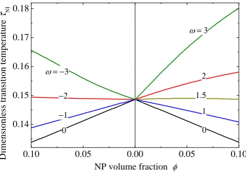
We first analyze the effect of NPs on the isotropic-nematic transition temperature. Typical profiles of the calculated transition temperatures as functions of the NP volume fraction are presented in Fig. 1 forξ= 0.5, i.e., the NP volume is twice larger than the LC molecular volume. Note that the transition temperatures for particles with negative and positive anisotropy are presented on the left and on the right hand side of the chart, respectively. One can readily see that the TN I(φ) variations are almost linear, which

is very similar to the experimental results in Ref. 21 and the analytical Eq. (23). For smaller ω, the addition of NP results in a decrease of the transition temperature, i.e., the effect of LC dilution prevails. For the values

12 M.A. Osipov and M.V. Gorkunov

0 . 0 0 0 . 0 5 0 . 1 0 0 . 1 0 0 . 0 5

0 . 1 4 0 . 1 5 0 . 1 6 0 . 1 7 0 . 1 8

0 1 1.5 2

= 3

D

im

en

si

o

n

le

ss

t

ra

n

si

ti

o

n

t

em

p

er

at

u

re



0 −1 −2

N P v o l u m e f r a c t i o n 

= −3

Fig. 1. Isotropic-nematic transition temperature as a function of the NP volume fraction for several negative (on the left) and positive (on the right) values of the NP anisotropy ω. Note the reversed direction of theφ-axis on the left

Typical variations of the transition temperature as functions of the NP anisotropy are presented in Fig. 2. It can be seen that even far beyond the limit of the weak NP anisotropy, the curves still correspond to the approximately parabolic dependence on W of Eq. (23). For larger NP concentrations the effect of NPs is more pronounced. According to Fig. 1, in the region of smallωthe NPs again effectively dilute the LC. At stronger anisotropy, the NPs make a positive effect on the nematic and increase its temperature range. The intersections of different curves take place at the points, which correspond to the lines ω =−2 and ω = 1.5 in Fig. 1. The points on these lines correspond to the values of parameters for which the effect of dilution is compensated by that of the anisotropy and as a result the transition temperature is practically independent of φ.

- 3 - 2 - 1 0 1 2 3 0 . 1 4 0

0 . 1 4 5 0 . 1 5 0 0 . 1 5 5 0 . 1 6 0 0 . 1 6 5

= 0 . 0 5 0 . 0 3 0 . 0 2 0 . 0 1

D

im

en

si

o

n

le

ss

t

ra

n

si

ti

o

n

t

em

p

er

at

u

re



S t r e n g t h o f a n i s o t r o p i c i n t e r a c t i o n s



Fig. 2. Isotropic-nematic transition temperature as function of nanoparticle anisotropy for several values of nanoparticle concentrationφ.

Therefore the nematic ordering improves and the transition temperature in-creases. At certain values of the NP anisotropy this effect can compensate the negative ”dilution” effect, and then the main LC thermodynamic prop-erties remain almost constant independently of the NP concentration. In general, the behavior of a particular composite material is determined by the competition of ”dilution” and ”orientation” effects.

2.4. Softening of the first order N-I transition

Let us now consider the temperature profiles of the LC order parameterS

and NP order parameterSp. As shown in the previous subsection, for small

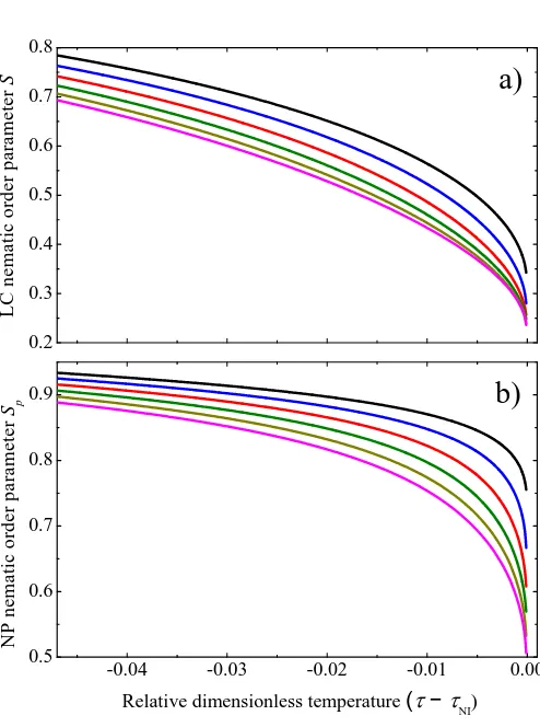
anisotropy, the presence of NPs mainly results in a renormalization of the transition temperature, while the nematic order parameter S does not ex-perience any qualitative changes. In contrast, for stronger NP anisotropy, NPs may significantly affect the transition scenario. Several examples of such behavior are shown in Figs. 3 and 4, where the profiles are presented for

ω= 3 andω=−3, respectively, and for several values of the concentration

14 M.A. Osipov and M.V. Gorkunov

0 . 2 0 . 3 0 . 4 0 . 5 0 . 6 0 . 7 0 . 8

- 0 . 0 4 - 0 . 0 3 - 0 . 0 2 - 0 . 0 1 0 . 0 0

0 . 5 0 . 6 0 . 7 0 . 8

0 . 9

b )

L

C

n

e

m

a

ti

c

o

rd

e

r

p

a

ra

m

e

te

r

S

a )

R e l a t i v e d i m e n s i o n l e s s t e m p e r a t u r e ( −_{N I})

N

P

n

e

m

a

ti

c

o

rd

e

r

p

a

ra

m

e

te

r

Sp

Fig. 3. Temperature dependencies of the nematic order parameters of LC (a) and NP (b) forξ= 0.5,ω= 3 andφ= 0,0.02,0.04,0.06,0.08,0.1 (from the upper to lower curves respectively).

a second order phase transition.

Comparing the behavior of S and Sp one concludes that they tend to

follow qualitatively the proportionality given by Eq. (21). The latter can-not be applied here directly, but the main features remain valid: largerS

corresponds to larger|Sp|, and sign reversal ofωreverses the sign of Sp.

0 . 0 0 . 1 0 . 2 0 . 3 0 . 4 0 . 5 0 . 6 0 . 7 0 . 8

- 0 . 0 4 - 0 . 0 3 - 0 . 0 2 - 0 . 0 1 0 . 0 0

- 0 . 5 - 0 . 4 - 0 . 3 - 0 . 2 - 0 . 1 0 . 0

L

C

n

e

m

a

ti

c

o

rd

e

r

p

a

ra

m

e

te

r

S

b )

a )

R e l a t i v e d i m e n s i o n l e s s t e m p e r a t u r e (

-

N

P

n

e

m

a

ti

c

o

rd

e

r

p

a

ra

m

e

te

r

Sp

Fig. 4. The same as in Fig. 3 for the negative NP anisotropyω=−3.

recently in the theory of biaxial nematics.38 Therefore one expects that this may be a general feature of the nematic-isotropic phase transition in sys-tems with additional degrees of freedom, which can be modified/ordered by the conventional uniaxial nematic ordering. Such a softening of the nematic-isotropic transition has not been described in Ref. 11 because the phenomenological theory developed there accounts for the orientational or-der of the NPs only to the lowest oror-der.

2.5. Comparison with existing experimental data

16 M.A. Osipov and M.V. Gorkunov

the main established facts. For example, the “dilution”-type decrease of the transition temperature has been found in nematic LC polymers doped with isotropic (at least on average) silver NPs (see Fig. 3 of Ref. 21), in a typical nematic LC doped with gold NPs with the diameter of 3–5 nm and volume fraction of 10−4−10−3 (see Table of Ref. 22), in LCs doped with spherical aerosil particles23,24_{and in dye doped nematics and polymer} dispersed nematic LCs (see Table 1 of Ref. 39).

An example of substantially anisotropic NPs are carbon nanotubes which are known to promote the nematic order and increase the transi-tion temperature.25 _{The increase of the N-I transition temperature by} 3-4 degrees has also been observed in nematics doped with large magnetic nanorods of the average diameter of 40 nm and the average aspect ratio of 10 (see Table 1 of Ref. 26). Also it has been shown experimentally that fer-roelectric Sn2P2S6 or BaTiO3 nanoparticles at low concentration (< 1%) enhance the orientational order parameter of the host liquid crystal and increase the transition temperature by about 5 K.9,10

Very recently a detailed experimental study of the effect of the shape anisotropy of magnetic NPs on the N-I phase transition has been under-taken40 _{inspired by the theoretical results presented in Ref. 27. The LC} was doped with spherical and rod-like magnetic particles of different size and the measurements have been made for different volume concentrations of NPs. It has been shown that the variation of the phase transition tem-perature with the increasing the NP concentration depends significantly on the NP shape anisotropy. In full agreement with the theoretical conclusions presented above, ferronematics doped with rod-like magnetic NPs are char-acterized by a higher NI transition temperature TNI in comparison with the host nematic or the same nematic LC doped with spherical NPs.

In Ref. 41, the effects of the cis and trans forms of

3. Nematic-isotropic separation in liquid crystals doped with spherical nanoparticles

3.1. Simple Molecular theory

Let us consider a nematic LC doped with small amount of spherical NPs. In the appropriate molecular theory one has to take into account both isotropic and anisotropic interactions between LC molecules, isotropic interactions between LC molecules and spherical NPs, and also isotropic interactions between NPs themselves.33 Then the system can be characterized by the following total interaction potential averaged over all molecule/particle po-sitions:

H= 1

2

X

ij

[Vmm(ai·aj) +Unn+Unm+Umm], (28)

where Unn, Umm and Unm are the average isotropic interaction potential

between NPs , LC molecules and between a NP and a LC molecule, re-spectively. Vmm(ai·aj) is the anisotropic interaction potential between LC

molecules which depends on the unit vectors ai and aj in the direction of

the primary axis of the molecules iandj, respectively.

In the mean field approximation, the free energy of the nematic phase can be written in the form (see, for example, Ref. 42).

1

VFN=kBT ρn(lnρn−1) +kBT ρm(lnρm−1)

−1

2ρ 2

nUnn−

1 2ρ

2

mUmm+ρmρnUmn

+1 2ρ

2

m Z

Vmm(ai·aj)fm(ai)fm(aj)daidaj

+kBT Z

fm(a) lnfm(a)da, (29)

where fm(a) is the orientational distribution function of the mesogenic

molecules, and ρm and ρn are the number densities of the mesogenic

molecules and NPs correspondingly.

The function Vmm(ai·aj) can be expanded in Legendre polynomials Pn(ai·aj) taking into account the first nonpolar term which is responsible

for the nematic ordering:

Vmm(ai·aj)≈U0+J P2(ai·aj). (30)

18 M.A. Osipov and M.V. Gorkunov

Substituting this expansion into Eq. (29) one obtains the following Maier-Saupe type free energy of the nematic composite:

1

VFN=kBT ρn(lnρn−1) +kBT ρm(lnρm−1)

−1

2ρ 2

nUnn−

1 2ρ

2

mUmm+ρmρnUmn

+1 2ρ

2

mJ S

2_k

BT Z

fm(a) lnfm(a)da, (31)

where S is the nematic order parameter of the mesogenic molecules which is expressed as:

S=

Z

P2(a·n)fm(a)da, (32)

where n is the nematic director. Minimizing the free energy (31) with respect to the orientational distribution function fm(a) and substituting

the equilibrium expression forfm(a) back into Eq. (31) one obtains:

1

VFN=kBT ρn(lnρn−1) +kBT ρm(lnρm−1)

−1

2ρ 2

nUnn−

1 2ρ

2

mUmm+ρmρnUmn−

1 2ρ

2

mJ S

2

−kBTlnZ, (33)

where

ZN =

Z π

0

exp[−βρmJ SP2(cosγ)] sinγdγ, (34)

and where the nematic order parameter S satisfies the following self-consistent equation:

S= 1

ZN

Z π

0

P2(cosγ) exp[−βρmJ SP2(cosγ)] sinγdγ, (35)

The free energy of the isotropic phase is obtained by settingS= 0:

1

VFI=kBT ρn(lnρn−1) +kBT ρm(lnρm−1)

−1

2ρ 2

nUnn−

1 2ρ

2

mUmm+ρmρnUmn. (36)

3.2. Nematic-isotropic phase separation

isotropic phases in the system under consideration is possible only if the chemical potentials of both NPs and mesogenic molecules are the same in the two phases. The pressure must also be the same in the two phases. How-ever, for incompressible LCs only the equations for the chemical potentials are relevant that isµnI =µnN andµmI=µmN whereµnIandµnN are the

chemical potentials of the NPs in the isotropic and in the nematic phase, respectively, and µmI andµmN are the corresponding chemical potentials

of the mesogenic molecules.

Using the well known general equation for the chemical potential one obtains the following system of two simultaneous equations

1

VI

∂FI

∂ρn

= 1

VN

∂FN

∂ρn

, 1

VI

∂FI

∂ρm

= 1

VN

∂FN

∂ρm

. (37)

Substituting Eqs.(36) and (33) for the free energies of the isotropic and the nematic phase into (72) one obtains the following equations:

lnρmN

ρmI

=U1(ρmN −ρmI) +U12(ρnN−ρnB) + lnZN, (38)

and

lnρnN

ρnI

=U2(ρnN−ρnI) +U12(ρmN−ρmI), (39)

where we have introduced the non dimensional interaction constants U1= Umm/(kTB),U2=Unneff/(kTB),U12=Unmeff/(kTB) and the number densities

of the mesogenic molecules, ρmI and ρmN, and NPs,ρnI andρnN, in the

isotropic and nematic phases correspondingly.

Neglecting a small density change at the transition, the number densities of both NPs and mesogenic groups in the nematic and in the isotropic phase can be expressed in terms of the volume fraction φi of NPs in the

corresponding phasei:

ρni=ρn0φi, ρmi=ρm0(1−φi), (40)

where i =N, I, ρm0 is approximately equal to the number density of the mesogenic groups in the pure LC and ρn0 can be estimated asρn0∼1/vp

where vp is the NP volume.

Now Eqs. (38) and Eqs. (39) can be expressed in terms of the two variablesφN andφI:

ln1−φN 1−φI

=w1(φI−φN) + lnZN, (41)

ln φI

φN

20 M.A. Osipov and M.V. Gorkunov

where

w1= (ρm0U1−ρn0U12), w2= (ρn0U2−ρm0U12). (43)

One notes that Eqs. (41) contain only two constants w1, w2, and it can readily be shown that the phase coexistence is possible only ifw2>1. If the isotropic attraction between NPs and mesogenic molecules is much stronger than that between the mesogenic molecules, the inequalityρn0U12> ρm0U1 is satisfied and hence w1<0.

Numerical solution of Eqs. (41,42) together with Eq. (34) and the self-consistent Eq. (35) for the nematic order parameter is significantly simpli-fied if the volume fraction of NPs is sufficiently small in both phases, that isφI 1 andφN 1. In this case Eq. (41) is simplified as:

(1−w1)(φI −φN) = lnZN, (44)

One notes also that the partition function ZN is independent of φI, and

thereforeφI can be excluded from the system of simultaneous equations for φI 1 andφN 1 which results in a single equation for φN:

Zw2/(1−w1)

N = 1 +

lnZN

φN(1−w1)

(45)

NowφN can be found by solving Eq. (45) numerically, and φI can then be

evaluated in terms ofφN as:

φI =φN+

lnZN

1−w1

(46)

Naturally, the volume fractions of NPs in the nematic and the isotropic phases are not completely independent. Indeed, in the experiment one normally controls the total number of NPsNnin the volumeV which yields

the average volume fraction of NPs φ. It follows from the conservation of the total number of NPs that φV =φIVI+φNVN where V =VI +VN is

the total volume of the system. On the other hand, solutions of the Eqs. (41) and (42) are independent ofφ. From these equations one obtains the following expressions for the volumesVN and VI:

VI =V

φ−φI

φI−φN

, VN =V

φN −φ

φI−φN

. (47)

One can readily see from Eqs. (47) that the phase coexistence is possible only ifφN < φ < φI as φN < φI. Taking into account thatφN andφI are

independent ofφ, one concludes that ifφis outside the interval (φN, φI), the

temperature. This condition should be used as an additional constraint imposed on the solutions of the Eqs. (41) and (42).

Finally, coexisting nematic and isotropic phases are globally stable only if the total free energy of the phase-separated system is lower than the free energy of both isotropic and nematic homogeneous phases. This is the second independent condition which should be taken into account in the consideration of the physical meaning of the formal solutions of the Eqs. (41) and (42) This condition can be expressed as:

F_{N I}sep−Fhom

V kBT

= 1

V kBT

_V

I

V FI(φI) +

VN

V FN(φN)−FI,N(φ)

<0, (48)

whereVI andVN are given by Eq. (47) and the free energy densitiesFI(φ)

and FN(φ) can be expressed using Eqs. (33, 36, 40):

FI(φ)/V kBT =ρn0φlnφ+ρm0(1−φ) ln(1−φ)

−1

2ρ 2

n0φ 2_U

2− 1 2ρ

2

m0(1−φ) 2_U

1+ρm0ρn0φ(1−φ)U12, (49)

FN(φ)/V kBT =FI(φ)/V kBT

−1

2ρ 2

m0(1−φ) 2_J∗_S2

m−ρm0(1−φ) lnZN, (50)

where J∗ _{= J/k}

BT. Note that for the separated state in Eq. (48) the

nematic order parameter is S(φN) in the nematic phase, which coexists

with the isotropic one, and is given by Eq. (35) withρm=ρm0(1−φN) and ZN =ZN(φN). At the same time, the order parameter of the homogeneous

nematic phase S(φ) is given by the same equation with ρm =ρm0(1−φ) and ZN =ZN(φ).

3.3. Phase diagrams

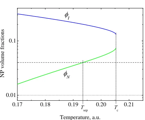
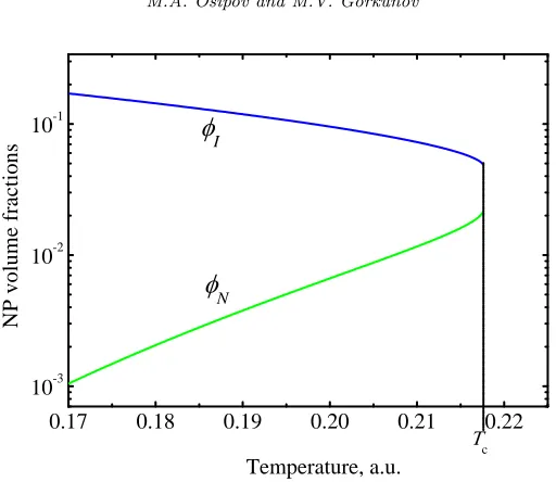
Let us first consider Eqs. (41) and (42) which enable one to determine the molar fractions of NPs in coexisting phases as functions of temperature. A typical numerical solution of these equations for moderately strong inter-actions between NPs and mesogenic molecules is presented in Fig. 5 One notes that there exists a bifurcation point which corresponds to a critical temperature Tc. At higher temperatures there is no solution, that is the

22 M.A. Osipov and M.V. Gorkunov

0 . 1 7 0 . 1 8 0 . 1 9 0 . 2 0 0 . 2 1

0 . 0 1 0 . 1

c s e p

N

P

v

o

lu

m

e

fr

ac

ti

o

n

s

T e m p e r a t u r e , a . u .





Fig. 5. Nanoparticle volume fractions in coexisting isotropic (upper curve) and nematic (lower curve) phases of the composites withw1=−5,w2= 10

It should be noted, however, that in the general case only part of this solution corresponds to an actual physical state of the system. As discussed in the previous subsection, Eqs. (41) and (42) do not depend on the average molar fraction of NPsφwhich can be actually controlled in experiments. At the same time, the value ofφmust lie between the two branches in Fig. 5, as

φN < φ < φI. Ifφis different from the critical value ofφcat the bifurcation

point, the system separates into the nematic and the isotropic phases with finite difference of NP molar fractions and finite volumes of both phases. In this general case the separation occurs at some temperature Tsep which

is below the bifurcation temperature Tc, and which is an intersection of

the horizontal line φ and one of the curves representing φN(T) or φI(T)

(see the intersection of φN(T) and the horizontal dashed line φ= 0.04 in

Fig. 5).

In principle, even if T < Tsep one cannot finally conclude that the

0 . 0 0 0 . 0 2 0 . 0 4 0 . 0 6 0 . 0 8 0 . 1 0 0 . 1 7

0 . 1 8 0 . 1 9 0 . 2 0 0 . 2 1 0 . 2 2 0 . 2 3

∗

T

em

p

er

at

u

re

,

a.

u

.

N P v o l u m e f r a c t i o n

N

P h a s e s e p a r a t e d

I

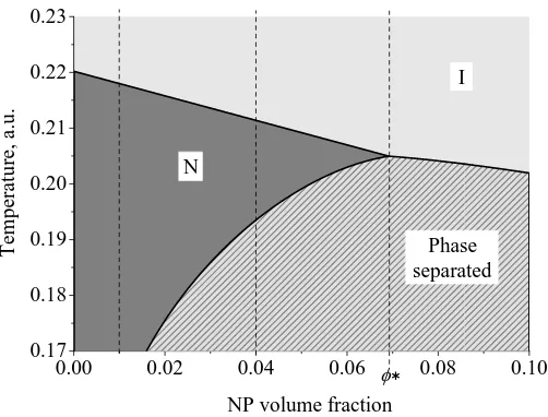
Fig. 6. Phase diagram of the composite calculated from the mean-field theory with interaction constantsw1=−5 andw2= 10.

therefore, the system never phase separates.

The solutions forφN and φI together with Eq. (48) have been used to

compose the temperature-concentration phase diagram presented in Fig.6 for the same values of the interaction constantsw1andw2as in Fig. 5. One notes that there is no phase separation at sufficiently low concentration of NPs. In this domain, the N-I transition temperature decreases with the increasing φ due to the “dilution” effect considered in Section 2. Above a certain critical concentration, the N-T phase transition is accompanied by the separation between the isotropic and the nematic phase, and the two phases coexist over a significant temperature interval. In this region the transition temperature into the phase-separated state decreases more slowly than the N-I transition temperature at low concentrations. It is interesting to note also, that in this case there exists another critical value

φ∗ of the NP molar fraction shown in Fig. 6. When φ > φ∗, the system undergoes a direct transition from the isotropic into the the phase separated state in which the isotropic and the nematic phases coexist. In contrast,

whenφ < φ∗, the system first undergoes a transition into the homogeneous

24 M.A. Osipov and M.V. Gorkunov

0 . 1 7 0 . 1 8 0 . 1 9 0 . 2 0 0 . 2 1 0 . 2 2 1 0 - 3

1 0 - 2 1 0 - 1

N

P

v

o

lu

m

e

fr

ac

ti

o

n

s

T e m p e r a t u r e , a . u .





_c

Fig. 7. The same as in Fig. 5 withw1=−10 andw2= 30

In this case the temperature range of the coexistence between the nematic and the isotropic phase is more narrow, and there is only a relatively small window of NP concentration when the separation takes place at all. One notes also, that in this case a reentrant homogeneous nematic phase may occur within a narrow interval of NP molar fraction.

On the other hand, for weaker interactions between NPs and meso-genic molecules (smaller absolute values of w1), the region of phase sep-arated state expands considerably (compare Figs. 6 and 9). Decreasing

|w1| results in a proportionate decrease of the critical total concentration φ∗. Additionally, in this case the phase separated state dominates over the low-temperature part of the phase diagram and even at small total NP concentrationsφthe homogeneous nematic phase exists only in a finite temperature range as illustrated by Fig. 9.

suf-0 . suf-0 suf-0 0 . 0 2 0 . 0 4 0 . 0 6 0 . 0 8 0 . 1 0 0 . 2 0

0 . 2 1 0 . 2 2

P h a s e s e p a r a t e d

T

em

p

er

at

u

re

,

a.

u

.

N P v o l u m e f r a c t i o n

N

I

Fig. 8. The same as in Fig. 6 withw1=−10 andw2= 30

ficiently low concentration of NPs because the entropy of mixing dominates the behavior of the system. Moreover, within a certain range of concen-trations of NPs the composite may undergo a direct transition from the isotropic phase into the phase separated state, while at other concentra-tions of NPs the system first undergoes a transition into the homogeneous nematic phase and then into the phase separated state at lower tempera-ture.

This unexpected behavior of nematic nano-composites is related to the fact that the properties of NPs differ very much from those of typical meso-genic molecules. In particular, the isotropic interaction between NPs and mesogenic groups (and between NPs themselves) is expected to be signifi-cantly stronger than that between mesogenic molecules. This is mainly due to the large effective volume of a typical spherical NP which includes also organic chains attached to the surface of metal or semiconductor core.

26 M.A. Osipov and M.V. Gorkunov

0 . 0 0 0 . 0 2 0 . 0 4 0 . 0 6 0 . 0 8 0 . 1 0 0 . 2 0

0 . 2 1 0 . 2 2

∗

T

em

p

er

at

u

re

,

a.

u

.

N P v o l u m e f r a c t i o n

N

I

P h a s e s e p a r a t e d

Fig. 9. The same as in Fig. 6 withw1=−1 andw2= 10

experimentally that gold NPs with mesogenic coatings form reversible net-works composed of nematic droplets accompanied by disclination lines and loops as a result of a specific phase separation which results in an enrich-ment of the NPs at the nematic-isotropic liquid interfaces.

Finally it should be noted that the theory of phase separation in LC nano-composites is at its rudimentary stage and there is much to be done here. Recently phase separation effects in nematics doped with large col-loidal particles have been studied theoretically in Refs. 47–49. In particular, very broad N-I coexistence region has been found in Refs. 47,48 using sim-ple mean-field theory of mixtures. This theory, however, is based on a different (and rather oversimplified) model interaction potential which is more suitable for large colloidal particles.

4. Chain formation and dielectric anisotropy of nematic nanocomposites

4.1. Simple theory of chain formation

parallel to each other and to the interparticle vector r12. If this potential minimum is sufficiently deep, the NPs form polar chains which may signif-icantly contribute to the dielectric anisotropy of the nematic composite.

The nematic composite with chains of NPs is characterized by the dis-tribution of chain lengths which can be evaluated using the existing theory of chain formation in the system of polar spheres presented, for example, in Ref. 36. According to this theory, the number density of chains of length

l (i.e. composed ofl NPs) is expressed as:

φl=vpρl=el(U0+Λ)e−U0, (51)

where φl is the volume fraction of chains of lengthl,vp is the NP volume

and U0 is the contact energy determined by the dipole-dipole interaction between NPs:

U0= ln

_πσ3_e2λ

18vλ3

. (52)

Here λ=µ2_/k

BT σ3 and σ is the NP diameter and the NP volumev has

been introduced for dimensional correctness.

In Eq. (51), Λ is the Lagrange multiplier (chemical potential) which is determined from the conservation rule for NPs:

ρp=

∞

X

l=1

lρl, (53)

where, as above, ρp is the total NP number density which is controlled

experimentally.

Substituting Eq. (51) into Eq. (53) and performing the summation one obtains:

ρp=v−1p

eΛ

(1−eU0+Λ₎2. (54)

Accordingly,

1−eU0+Λ ₌−1 +

√

1 + 4η

2η , (55)

where η =vpρpeU0. Thus the value of the chemical potential Λ is mainly

determined by the order ofη.

Finally, one can readily obtain the following expression for the number density of chains of lengthl:

ρl=vp−1e

−U0

1−−1 + √

1 + 4η

2η

l

28 M.A. Osipov and M.V. Gorkunov

4.2. High frequency permittivity of a nematic composite

At sufficiently high (optical) frequencies the polarization is mainly deter-mined by induced dipoles created by the electric field. Orientational fluctu-ations of permanent dipoles make a minor contribution because the charac-teristic times of such fluctuations are much larger than the inverse optical frequency.50 _{Relatively simple explicit expressions for the dielectric} con-stant can be obtained in the molecular field approximation in the form of generalized Clausius-Mossotti relation51 _{assuming that the composite} nematic phase contains mesogenic molecules, NPs and chains of NPs of various lengthsl:

(ˆ−1)(ˆ+ 2)−1=4π

3 h

ˆ

βmiρm+hβˆnpiρnp+

∞

X

l=2

hβˆliρl !

, (57)

where hβˆmi, hβˆnpi and hβˆli are the average polarizabilities of mesogenic molecules, single NPs and chains of NPs of length l, respectively, and

ρm, ρnpandρl are the corresponding number densities.

Introducing the long axes of the moleculesam and the unit vectors of

the chain directions al, and using the corresponding scalar nematic order

parameters Sα one obtains the following expressions for the averaged

po-larizability tensors:

hβˆαi= ¯βαIˆ+Sα∆βαn⊗n, (58)

where the isotropic polarizabilities are expressed as ¯βα=βα⊥+ ∆βα(1−

Sα)/3.

Assuming that moderate dielectric anisotropies ∆βαgive rise to a

rela-tively small anisotropy of the composite permittivity ∆ε, Eq. (57) can be expanded and simplified as follows:

∆ε=4π

9 (ε⊥+ 2) 2 _∆β

mρmSm+

∞

X

l=2

h∆βliρl !

, (59)

while the isotropic part of the composite permittivity satisfies the scalar Clausius-Mossotti relation

ε⊥−1

ε⊥+ 2

= 4π

3 βm⊥ρm+βnpρnp+ ∞

X

l=2

βl⊥ρl

!

, (60)

indices of the nematic composite on the concentration of NPs, their aggre-gation and ordering provided that the effective polarizability of a NP in the nematic solvent is known.

4.3. Polarizability of a single chain

Generally, the NP contribution to the composite permittivity (59) and (60) is twofold: both aggregated and non-aggregated NPs affect ε⊥ while only those NPs which are aggregated into chains contribute to ∆ε.

To sum over chains of different lengths in Eq. (59) one needs to know the quantityh∆βliwhich can be evaluated as the average dielectric anisotropy of a chain ofl spheres (with the permittivityεnp) immersed into a medium

with the permittivity ε⊥. Although the exact solution of such a problems can be obtained only numerically, one can obtain useful analytical esti-mates52using a few realistic approximations. Thus taking into account the strongest dipole interactions between NPs and restricting the calculations to the nearest-neighbor contributions (already the next-nearest neighbor ones are at least eight times smaller) and introducing the single NP dielec-tric polarizability β1 = 1/8 σ3(εnp−ε⊥)/(εnp+ 2ε⊥) one can express the dipole moment of thek-th NP in the chain of the total lengthlas

pk =β1E+β1Tˆk,k−1pk−1+β1Tˆk,k+1pk+1, (61)

where

ˆ

Tk,k±1= (3uk,k±1⊗uk,k±1−1)σ−3, (62) is the non-singular part of the dipole-dipole propagator,uk,k±1are the unit vectors between the centers of the adjacent NPs and the following natural condition is satisfied ˆT1,0= ˆTl,l+1= 0 at the chain ends.

As shown below, the effect of chain formation on high-frequency permit-tivity is rather moderate, and one can solve the system (61) by iterations. While in the zeroth order (neglecting the NP interactions) one obtains merely pk =β1E and the chain remains dielectrically isotropic, the next iteration yields:

pk =β1

1 +β1Tˆk,k−1+β1Tˆk,k+1

E. (63)

Since the average chain direction is controlled by the overall composite nematic director n, the averaged nearest-neighbor propagator reads

30 M.A. Osipov and M.V. Gorkunov

where we have again assumed that all the scalar nematic order parameters in the composite are equal.

Evaluating the average chain dipole moment as hPli=Pl

k=1hpkione obtains the following expression for the overall average chain polarizability tensor

hβˆli=lβ11+ 2

σ3(l−1)β

2

1S(3n⊗n−1). (65)

The anisotropy of this polarizability is given by:

h∆βli= 6

σ3(l−1)β

2

1S. (66)

4.4. Contribution of polar chains to the dielectric anisotropy

of the nematic composite

Accordingly, the chain contribution to the composite permittivity anisotropy (59) is given by

∆εch= π

24

_(ε

⊥+ 2)(εnp−ε⊥)

εnp+ 2ε⊥

2

Sσ3

∞

X

l=2

(l−1)ρl. (67)

Substituting the number densities (56) an using the summation rule

∞

X

l=2

(l−1)xl= x 2

(1−x)2 (68)

one can express the dielectric anisotropy in terms of the dimensionless NP densityρ∗_=ρσ3 _{and the parameterλ:}

∆εch= π

24

_(ε

⊥+ 2)(εnp−ε⊥)

εnp+ 2ε⊥

2

Sρ∗δη. (69)

where the function

δη= 2 +

1

η −

4η

(√1 + 4η−1)2 (70)

effectively describes the dependence on the NP chain formation as η

is also expressed in terms of the non-dimensional parameters as η =

πρ∗e2λ_/(18λ3_).

Representative profiles of the factorδη as functions of the NP coupling

2 4 6 8 1 0 1 0 - 3

1 0 - 2 1 0 - 1 1 0 0

0 . 0 0 1 0 . 0 1

∗

= 0 . 1



N P d i p o l e i n t e r a c t i o n s t r e n g t h , 

Fig. 10. The effect of chain formation on the high-frequency dielectric anisotropy of the composite: dependences of the factorδαgiven by Eq. (70) on the NP coupling strength for NP densitiesρ∗= 0.1, 0.01 and 0.001 as indicated on the lines.

increase of the anisotropy. The saturation atδη≈1 for strongly interacting

NPs means that in this limit practically all NPs belong to long chains and contribute equally to the anisotropy. Evidently, for higher total NP concentrations this saturation occurs at smaller λ.

The variation of the high frequency dielectric anisotropy as a function of the NP concentration is illustrated by Fig. 11 for different values of the dipole-dipole interaction strength. One notes that this variation is approximately linear when the NP coupling is strong enough, i.e., when all the NPs are aggregated in long chains.

Generally, the high-frequency anisotropy is weak as the factor δη <1

is multiplied in Eq. (69) by a number of other small factors. Thus for the dielectric NPs withεnpof the same sign and order of magnitude as ε⊥ the factors in the square brackets are of the order of unity, while S < 1 and

ρ∗_{1. On the other hand, the variation ofδ}

ηby three orders of magnitude

for lowρ∗= 0.001 in Fig. 10 suggests that this anisotropy can be employed as a sensitive tool for quantitative assessment of the NP chain formation in nematic composites.

4.5. Low frequency dielectric constant of a strongly polar

nematic composite

fluc-32 M.A. Osipov and M.V. Gorkunov

0 . 0 0 0 . 0 2 0 . 0 4 0 . 0 6 0 . 0 8 0 . 1 0 0 . 0 2

0 . 0 4 0 . 0 6 0 . 0 8 0 . 1 0

4

6

2

8

= 1 0



∗



N P d i m e n s i o n l e s c o n c e n t r a t i o n , ∗

Fig. 11. The effect of chain formation on the high-frequency dielectric anisotropy of the composite: dependences of the factorρ∗_δ

ηin Eq. (69) on the NP concentration for the coupling strengthλvarying from 2 to 10 as indicated on the lines.

tuations of permanent molecular dipoles while the molecular polarizability gives a much smaller contribution. Indeed, the static dielectric constant of a strongly polar nematic can be of the order of 100 while a typical con-tribution from the molecular polarizability is of the order of 3.50 _{In this} case, the macroscopic polarization can be expressed as a sum of averaged molecular dipoles of all components αof the mixture in the unit volume:

P=X

α

ραhµαi, (71)

where µα is the permanent molecule/particle dipole of the componentα.

In the static case, the average dipole can be expressed as:

hµαi= Z

µαfα(θ)dθ, (72)

where fα(θ) is the one-particle distribution function which can be written

in the following form in the mean-field approximation

fα(θ) =Z−1exp [−(UMF,α(θ) + (µα·E))/(kBT)]. (73)

Here UMF,α(θ) is the mean-field potential for the componentα,θ specifies

the orientation of the particle/molecule andEis the external electric field. The mean-field potential can be written in the form:

UMF,α(θ1) =

X

β Z

whereVα,β(θ1, θ2) is the pair interaction potential between the components

αandβ.

Let us now assume that both mesogenic molecules and NPs are uniaxial and their permanent dipoles are parallel to the corresponding long axes. This is also valid for rigid chains of spherical dipolar NPs. In this case, the pair interaction potential V depends on the unit vectors a1 anda2 in the direction of the long axes of the molecules “1” and “2”, respectively, and on the intermolecular vector r12, i.e. V(1,2) = V(a1,r12,a2). The pair potential can now be written as a sum of the nonpolar and the polar parts,

V(1,2) =Vnp(1,2) +Vdd(1,2), where the nonpolar potentialVnp(1,2) is an

even function of a1 and a2 and where the polar potential Vdd(1,2) is the

electrostatic dipole-dipole interaction potential which can be expressed as:

Vdd(1,2) =µ1·Fˆ(r12)·µ2, (75)

where the dipole-dipole propagator can be written in the form:

ˆ

F(r12) =

4π

3 δ(r12) + Θ(r12−D)( ˆI−3u⊗u)r −3

12, (76)

where u=r12/r12 and where Θ(r12−D) is a step function which is equal to unity if r12 > D and vanishes otherwise. One notes that the first term in Eq. (76) takes into account a singularity of the dipole-dipole potential at the origin (see a detailed discussion of the averaging of the dipole-dipole potential in Refs. 36,53).

Substituting Eq. (76) into Eqs. (75) and (74) and taking into account that the second term in Eq. (76) vanishes after integration over all u, one obtains the final expression for the mean-field potential:

UMF,α(θ) =Uα(0)(θ) +

4π

3 (µα·P), (77)

Finally this mean-field potential can be substituted into the orientational distribution function (73) and expanding it in powers of the small electric field Eand filed-induced polarizationPone obtains:

fα(θ)≈fα(0)

1 + 4π 3

µα·P

kBT

−µα·E

kBT

, (78)

where the nonpolar distribution function fα(0) is determined by the

nonpolar part Uα(0)(θ) of the mean field potential, that is f0,α =

Z₀−1exph−Uα(0)(θ)/(kBT)

i

34 M.A. Osipov and M.V. Gorkunov

Substituting Eq. (78) into Eqs. (72) and (71) one obtains the following linear equation for the macroscopic polarizationP:

Pi=

X

α

ρα

kBT

hµα,iµα,ji0

4π

3 Pj+Ej

, (79)

where the averaging hµα,iµα,ji0 is performed with the nonpolar orienta-tional distribution function fα(0). As a result, one obtains the following

expression for the dielectric polarizability tensor ˆχ:

ˆ

χ= χˆ0

1−4π

3χˆ0

(80)

where

ˆ

χ0=

X

α

ρα

kBT

hµα⊗µαi0. (81)

Taking into account that the dipole µαis parallel to the long axis aof the

corresponding molecule one obtains:

ˆ

χ0=

X

α

ραµ2α

kBT

ha⊗ai0=

X

α

ραµ2α

kBT

[Sα(n⊗n−1/3) +1/3]. (82)

HereSαis the nematic order parameter of the compoundαin the mixture.

Let us consider the nematic composite in which the permanent dipoles of NPs are sufficiently large and larger than those of the mesogenic molecules. Then the main contribution to the low frequency dielectric constant of the nano-composite stems from the NPs and their chains and can be written using Eq. (81) as:

ˆ

ε≈1 + 4πχˆ0= 1 + 4π ∞

X

l=1

ρlµ2l

kBT

[Sl(n⊗n−1/3) +1/3], (83)

whereµlis the total dipole of the chain of lengthl,ρlis the number density

of chains of lengthl andSl is the corresponding nematic order parameter.

One may assume that for short rigid chains of polar NPs the total dipole

µl=lµwhereµis the permanent dipole of a single NP. This assumption is

obviously not valid for long flexible chains. However, the concentration of such chains is exponentially small and we will see below that for realistic values of the NP dipole only short chains (l= 1−4) make a significant con-tribution to the dielectric constant of the composite. In this approximation Eq. (83) yields the dielectric susceptibility anisotropy:

∆χ= µ

2

kBT

X

l=1

1 0

1 0

1 0

2

4

6

8

1 0

1 0

1 0

1 0

1 0



/

S

b )



= 0 . 0 1

7

6

5

4

3

1

2



= 0 . 0 0 1

a )

N P d i p o l e i n t e r a c t i o n s t r e n g t h ,



/

S

7

6

5

4

3

1 2

Fig. 12. Anisotropy of the low-frequency composite dielectric susceptibility as a function of NP coupling strength for NP densitiesρ∗= 0.001 (a) andρ∗= 0.01 (b). Solid lines 1−6 depict results of partial summation in Eq. (84) neglecting chains withlhigher than 1−6 correspondingly. Solid line 7 represents the dependence (86), and the dashed line shows the anisotropy in the absence of chain formation.

By setting Sl=S and substituting the number densities (56) one can

perform the summation over chains of all lengths in Eq. (84). Indeed, using the summation rule

∞

X

l=1

l2xl= x(1 +x)

(1−x)3 (85)

the low-frequency dielectric anisotropy can be expressed explicitly in terms

ρ∗ andλ:

∆χ= 4ρ∗λS 4η

2_{+ 5η+ 1−(3η+ 1)}√_{1 + 4η}

−1 +√1 + 4η3 . (86)

36 M.A. Osipov and M.V. Gorkunov

0 . 0 2 0 . 0 4 0 . 0 6 0 . 0 8 0 . 1 0 1 0 - 3

1 0 - 2 1 0 - 1 1 0 0 1 0 1 1 0 2



/

S

N P d i m e n s i o n l e s c o n c e n t r a t i o n , ∗

4

6

2

8

= 1 0

Fig. 13. Anisotropy of the low-frequency composite dielectric susceptibility as a function of the NP concentration for the NP interaction strength λ varying from 2 to 10 as indicated on the lines.

we also present the corresponding variation ∆ ˜χ = λSρ∗ of the dielectric anisotropy of the composite without any chains, as well as the results of the partial summation in Eq. (84) which show the relative scale of contribu-tions from chains of different lengths. One can see that the chain formation can modify the dielectric properties by orders of magnitude when the NP interaction (determined by the permanent dipole) is sufficiently strong. At the same time, for weak interaction, the effect of chains is practically negli-gible and the NPs respond to the electric field independently. For moderate interactions, there exists a noticeable area ofλ, where the formation of short chains (dimers and trimers) contributes to ∆χconsiderably, while the effect of longer chains is practically absent.

One can readily see in Fig. 12 that the contributions from monomers and dimers (similar to that from monomers andl-mers forl= 3,4,5) first increases with the increasing dipolar strengthλ, then reaches a maximum and finally begins to decrease. The decreasing stage corresponds to the range ofλwhich correspond to the formation of longer chains which make a predominant contribution to the dielectric anisotropy. In this range the contribution from dimers, trimers etc. decreases due to a decrease of the corresponding number densities. The increasing stage corresponds to the range of smaller λwhere the corresponding short chains make a predomi-nant contribution.

concentration for different values of the dipole-dipole interaction strength is presented in Fig. 13. Evidently, the increase of the NP concentration by an order of magnitude results in the increase of the dielectric anisotropy by several orders of magnitude depending on the value of the parameter λ. Thus one can readily see (compare also with Figs. 12a and 12b) that the experimentally observed increase of the dielectric constant9,34 _{at very low} NP number densityρ= 10−2−10−3can be explained by the effect of chain formation only if the dipole-dipole interaction strength is sufficiently high which is the case for ferroelectric NPs with large spontaneous polarization. One notes that at present there is no direct experimental evidence of the existence of chains of NPs in nematic composites although a number of ex-perimental data cannot be explained without assuming that such chains are actually formed. Recently, however, it has been shown experimentally that in an isotropic fluid doped with an extremely low concentration of magnetic dipolar spherical NPs some birefringence can be induced by the external magnetic field.54 In such a fluid, the macroscopic magnetic anisotropy can only be determined by the orientational ordering of dimers of magnetic NPs induced by the external field, and theoretical estimates of dimer concentra-tion can be used to explain the experimentally observed dependence of the birefringence on the external magnetic field.54

5. Conclusions

38 M.A. Osipov and M.V. Gorkunov

NP concentration, on the measurements of orientational order parameter of anisotropic NPs and, in particular, on the experimental studies of phase separation effects for different molar fractions of NPs. Finally, some exper-imental methods should be found to study directly the chain formation in strongly polar nematic nano-composites.

Acknowledgments

The authors are grateful to J. Goodby, R. Richardson, N. Vaupotich, Yu. Reznikov, T.J. Sluckin, N. Tomasovicova, R.V. Talroze, A.A. Ezhov, A.S. Merekalov and Ya.V. Kudryavtsev for interesting discussions.

References

1. H. Qi, B. Kinkead, and T. Hegmann, Effects of functionalized metal and

semiconductor nanoparticles in nematic liquid crystal phases, Proc. SPIE.

6911, 691106 (2008).

2. H. Qi and T. Hegmann, Formation of periodic stripe patterns in nematic liquid

crystals doped with functionalized gold nanoparticles,J. Mater. Chem.16,

4197–4205 (2006).

3. Y. Shiraishi, N. Toshima, H. Maeds, K.and Yoshikawa, J. Xu, and S. Kobayashi, Frequency modulation response of a liquid-crystal electro-optic

device doped with nanoparticles,Appl. Phys. Lett.81(15), 2845–2847 (2002).

4. S. Kobayashi and N. Toshima, Nanoparticles and lcds: It’s a surprising world,

Information Display.23, 26 (2007).

5. H. Yoshida, K. Kawamoto, H. Kubo, A. Tsuda, T.and Fujii, S. Kuwabata, and M. Ozaki, Nanoparticle-dispersed liquid crystals fabricated by sputter doping,

Adv. Mater.22, 622–626 (2010).

6. S. Kaur, S. P. Singh, A. M. Biradar, A. Choudhary, and K. Sreeniva, Enhanced electro-optical properties in gold nanoparticles doped ferroelectric liquid

crys-tals,Appl. Phys. Lett.91, 023120 (2007).

7. A. Kumar, J. Prakash, A. M. Mehta, D. S.and Biradar, and W. Haase, Enhanced photoluminescence in gold nanoparticles doped ferroelectric liquid

crystals,Appl. Phys. Lett.95, 023117 (2009).

8. O. Buchnev, A. Dyadyusha, M. Kaczmarek, V. Reshetnyak, and Y. Reznikov, Enhanced two-beam coupling in colloids of ferroelectric nanoparticles in liquid

crystals,J. Opt. Soc. Am. B.24(7), 1512–1516 (2007).

9. Y. Reznikov, O. Buchnev, O. Tereshchenko, V. Reshetnyak, A. Glushchenko,

and J. West, Ferroelectric nematic suspension,Appl. Phys. Lett.82(12), 1917–

1919 (2003).

10. F. Li, C. Buchnev, O.and Cheon, A. Glushchenko, V. Reshetnyak, Y. Reznikov, T. Sluckin, and J. West, Orientational coupling amplification