CAMELOT - computational-analytical multi-fidelity low-thrust optimisation toolbox

CAMELOT - COMPUTATIONAL-ANALYTICAL MULTI-FIDELITY LOW-THRUST

OPTIMISATION TOOLBOX

Marilena Di Carlo, Juan Manuel Romero Martin, Massimiliano Vasile

Department of Mechanical and Aerospace Engineering, University of Strathclyde, Glasgow, UK

ABSTRACT

CAMELOT (Computational-Analytical Multi-fidelity Low-thrust Optimisation Toolbox) is a toolbox for the fast preliminary design and optimisation of low-thrust trajecto-ries. It solves highly complex combinatorial problems to plan multi-target missions characterised by long spirals including different perturbations. In order to do so, CAMELOT imple-ments a novel multi-fidelity approach combining analytical surrogate modelling and accurate computational estimations of the mission cost. Decisions are then made by using two op-timisation engines included in the toolbox, a single objective global optimiser and a combinatorial optimisation algorithm. CAMELOT has been applied to a variety of applications: from the design of interplanetary trajectories to the optimal deorbiting of space debris, from the deployment of constel-lations to on-orbit servicing. In this paper the main elements of CAMELOT are described and two space mission design problems solved using the toolbox are described.

Index Terms— Multi-target missions, low-thrust propul-sion, combinatorial problems, multi-fidelity, surrogate mod-els

1. INTRODUCTION

In recent years electric propulsion has become a key technol-ogy for space exploration and its use has increased in both near-Earth and interplanetary missions. Electric propulsion system have indeed the potential to provide shorter flight times, smaller launch vehicles and increased mass delivered to destination, when compared to high-thrust propulsion sys-tems [1, 2].

Electric propulsion multi-target missions have been pro-posed in the literature [3, 4] and they are typical problems of the Global Trajectory Optimisation Competition (GTOC), [5].

The design of such missions require the definition of the best sequence of targets to visit and therefore the solution of a combinatorial optimisation problem. An additional diffi-culty in solving large combinatorial problems is the need to evaluate the cost of the transfer between targets several times. To quickly solve these problems it is therefore desirable to have a fast estimation for the cost of the transfer. When the

model is expensive to evaluate, this estimation could be ob-tained through the use of surrogate models.

In this paper the Computational-Analytical Multi-fidelity Low-thrust Optimisation Toolbox (CAMELOT), a toolbox that combines the elements required to quickly design a low-thrust multi-target mission, is presented. CAMELOT includes multi-fidelity low-thrust transfer cost estimation, combinatorial optimisation solver, tools for the generation of surrogate models and single objective global optimiser. The combination of these elements allow to design a wide range of multi-target mission using electric propulsion: from the design of interplanetary trajectories to the optimal deorbiting of space debris, to the deployment of constellations.

In this paper two mission design applications of CAMELOT are presented: a multiple fly-by mission to the Atira astroids and an Active Debris Removal (ADR) mission to remove non-cooperative objects from Low Earth Orbit (LEO).

The paper starts with a description of the of the main tools of CAMELOT in Section 2. The two mission design applica-tions are described in Section 3 and final remarks conclude the paper.

2. CAMELOT

The main components of CAMELOT are:

- Fast Analytical Boundary-value Low-thrust Estimator (FABLE);

- Multi Population Adaptive Differential Evolution Al-gorithm (MP-AIDEA);

- Automatic Incremental Decision Making And Planning algorithm (AIDMAP).

2.1. FABLE

FABLE provides accurate cost estimations (∆V) of orbital transfers realized with electric propulsion using multi-fidelity analytical approach and surrogate models.

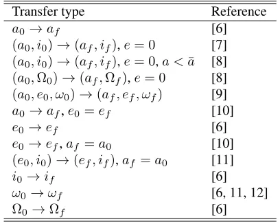
Table 1. Low-fidelity analytical control laws for the variation of orbital elements implemented in FABLE.

Transfer type Reference

a0→af [6]

(a0, i0)→(af, if),e= 0 [7]

(a0, i0)→(af, if),e= 0,a <¯a [8]

(a0,Ω0)→(af,Ωf),e= 0 [8]

(a0, e0, ω0)→(af, ef, ωf) [9] a0→af,e0=ef [10]

e0→ef [6]

e0→ef,af=a0 [10]

(e0, i0)→(ef, if),af =a0 [11]

i0→if [6]

ω0→ωf [6, 11, 12]

Ω0→Ωf [6]

The higher-fidelity approach computes the∆V using the analytical propagator implemented in FABLE. The analytical propagator is based on analytical formulas for the perturbed Keplerian motion obtained as results of a first-order expan-sion in the perturbing acceleration [13]. Using these formu-las, osculating analytical propagator and averaged analytical propagator are implemented in FABLE. They include pertur-bations due to J2 zonal harmonic, atmospheric drag (modelled using the exponential atmospheric density model [14]), solar radiation pressure and low-thrust propulsion. Analytical so-lution are available for constant low-thrust acceleration and for constant tangential low-thrust acceleration [13]. The ef-fect of shadow regions can also be included. Different control parameterisation can be implemented to compute low-thrust transfers.

When multi-target missions are considered the cost of the transfers between objects could have to be computed several times. In order to reduce the associated computational bur-den, FABLE can generate surrogate models of the transfers’ cost to allow for a fast evaluation of complex trajectories. Sur-rogate models can be obtained using Kriging and the DACE toolbox [15] and Tchebycheff interpolation with sparse grid [16].

FABLE includes also tools for multi-fidelity optimisation of surrogate models. The optimisation is realized using the concept of co-Kriging and the maximisation of the expected improvement. The co-Kriging model allows to build an ap-proximation of a function that is expensive to evaluate us-ing data from low-fidelity model of the function [17]. The high-fidelity responseZHF(x)is approximated by multiply-ing the low-fidelity responseZLF(x)by a scaling factor,ρ, and a Gaussian process representing the difference between the high and low-fidelity data,ZD(x), [18]:

ZHF(x) =ρZLF(x) +ZD(x) (1)

In FABLE the co-Kriging model is computed using ooDACE Toolbox [19].

The maximum expected improvement approach is used to locate the minimum of the function by finding the point where the likelihood of achieving an improvement, with respect to the current best function value, is maximized [20]. The ex-pected improvementEIis defined as:

EI =s(x) [uΦ (u) +φ(u)] (2)

where

u=fmin−yd(x)

s(x) (3)

In the previous equationyd(x)is the co-Kriging predictor,

s(x)is its error,Φandφare the normal cumulative distribu-tion funcdistribu-tion and density funcdistribu-tion andfminis the current best

function value [20].

FABLE includes also astrodynamics tools for gravity as-sist, as shown in Section 3. Additional analytical capabilities include the possibility to compute the energy of the spacecraft subject to J2 and solar radiation pressure perturbations.

2.2. MP-AIDEA

MP-AIDEA has been extensively tested over more than fifty test functions, including difficult academic test functions and real world test problems. Results have shown that the algorithm is averagely very efficient, being always in the first four positions in the ranking obtained comparing its results to those of others algorithms [22].

2.3. AIDMAP

The Automatic Incremental Decision Making And Planning algorithm (AIDMAP) is a single objective incremental de-cision making algorithm for the solution of complex com-binatorial optimisation problems such as tasks planning and scheduling. AIDMAP works modeling the discrete decision making problems into a decision tree where nodes represent the possible decisions while links/edges represent the cost vector associated with the decisions. AIDMAP incrementally builds the decision tree from a database of elementary build-ing blocks. These blocks represent a phase or leg of the mis-sion. Using this approach eases the transcription of the prob-lem into a tree-like topology. In addition, by incrementally building the decision tree, it is possible to prune the search space like proposed in [25, 26]. The decision tree is incre-mentally grown or explored by a set of Virtual Agents (VAs). The resulting decision tree is then evaluated by the VAs us-ing a set of deterministic or probabilistic heuristics. The de-terministic heuristics in AIDMAP are derived from classi-cal Branch-and-Cut [27, 28] while the probabilistic heuris-tics are bio-inspired and mimic the evolution of the slime mold Physarum Polycephalum, a simple single cell organ-ism endowed by nature with a simple but powerful heuris-tic that can solve complex discrete decision making problems [29, 30, 31]. Unlike Branch-and-Cut, that uses a set of de-terministic branching and pruning heuristics, the Physarum algorithm uses probabilistic heuristics to decide to branch or prune a vein. Branches are never really pruned but the prob-ability of selecting them may fall to almost zero. The mecha-nism of Physarum is analogous to the most commonly known Ant Colony Optimisation algorithm [30]. A more detailed description of the Physarum is given in [32].

AIDMAP has been extensively tested on a variety of Travelling Salesman and Vehicle Routing problems, provid-ing good results [14, 32, 33].

3. APPLICATIONS

CAMELOT can be applied to different mission design prob-lems. Here, a multiple asteroid fly-by mission and a multiple active debris removal mission are presented.

3.1. Multiple asteroids fly-by mission

The first application of CAMELOT is the design of a mission to visit the Atira asteroids [34]. Atira asteroids are Near-Earth

Asteroids (NEAs) with both perihelion and aphelion within the orbit of the Earth (semimajor axisa <1 AU and aphelion

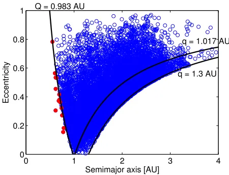
Q <0.983 AU), also called Inner-Earth Objects (IEOs). The first Atira object was discovered in 2003 and, as of December 2014, only fourteen asteroids are counted in this group. However, many more objects are expected to exist in the same region of the Solar System. To date, over eleven thousand NEAs have been identified, the majority of which are characterized by semimajor axis greater than 1 AU, as shown in Figure 1, where the distribution of the known NEAs is shown in thea-eplane, with the Atira asteroids represented in red. Inner Solar System asteroids are difficult to detect be-cause of the limitations of ground-based survey: telescopes can only search on the night side of the Earth, where the Sun is not in the field of view.

0 1 2 3 4

0 0.2 0.4 0.6 0.8 1

Semimajor axis [AU]

Eccentricity

Q = 0.983 AU

q = 1.017 AU

q = 1.3 AU

Fig. 1. NEAs distribution - red circles indicate Atira asteroids.

The proposed mission visits the Atira asteroids by making use of an electric propulsion system. To maximize the scien-tific return of the spacecraft, the mission is optimized to visit the maximum possible number of asteroids of the Atira group. The encounters with the asteroids are realized through a se-ries of fly-bys at the nodal points of their orbits. This strategy allows avoiding out-of-plane maneuvers for the change of in-clination; the 14 Atira asteroids have inclination ranging from 0 to 30 degrees.

The design of the mission is divided into three phases:

1. Identification of the optimal asteroid sequence and the optimal departure and arrival dates, using AIDMAP and an impulsive Lambert model for the transfer;

2. Refinement of the optimal solution identified by AIDMAP using MP-AIDEA;

In the first step AIDMAP is used to identify the optimal sequence of asteroids to visit and the optimal departure and arrival dates, considering a 10 years mission time span from 01 January 2020 to 01 January 2030. The trajectories between asteroids are composed of sequences of conic arcs linked to-gether through discrete, instantaneous events. Each conic arc is the solution of a Lambert problem, which is solved to com-pute the∆V required for the transfer to reach each asteroid at its nodal point. The arrival conditions are defined by the passage of the asteroids through their nodal points and the departure conditions are identified, on the departure orbit, by a minimum and maximum value for the time of flight to reach the nodal point, [34]. AIDMAP identifies 133,761 possible solutions. A filtering process is applied to identify solutions with different sequence of targeted asteroids. After the filter-ing, fourteen unique solutions visiting six asteroids and fifty-seven unique solutions visiting five asteroids are found. The best solution found by AIDMAP, that is the one characterized by the maximum number of asteroid visited and the lowest total∆V, has six fly-bys based on the following sequence of asteroids visited: Earth 2013JX28 2006WE4 2004JG6 -2012VE46 - 2004XZ130 - 2008UL90 . The total∆V cost, obtained from a Lambert model, is 3.77 km/s and the trans-fer time is 8.4 years. More details about this solutions are reported in Table 2.

The best solution identified by AIDMAP is then further optimized using the global optimiser MP-AIDEA. For the ad-ditional optimisation, a local window of 10 days is allocated around the previous defined departure dates in order to iden-tify new departures dates leading to an improved result in term of total∆V. The obtained results are reported in Table 3, showing a reduction of 0.16 km/s in the total∆V with re-spect to the results presented in Table 2.

In the last phase of the mission design FABLE is used to optimise the low-thrust transfer between the previously de-fined asteroids nodes. A direct optimisation method and mul-tiple shooting algorithm are used. In the mulmul-tiple shooting algorithm, the trajectory is segmented into legs that begin and end at On/Off control nodes, where On nodes define the switching point from null thrust to maximum thrust and Off nodes define the switching point from maximum thrust to null thrust The state vectors corresponding to each node are deter-mined by the optimisation process, being treated as optimis-ables controls [35]. The trajectory is therefore segmented into a sequence of thrust and coast legs. A middle point is defined for each transfer and the state vector is forward-propagated on each of the legs from the departure point to the mid point and back-propagated on each of the legs from the arrival point (that is, the asteroid nodal point) to the mid point. Keplerian motion is considered on the coast legs, while on the thrust legs the analytical model for the propagation of the orbital motion under low-thrust perturbation included in FABLE is used. The initial acceleration is set at10−4_m/s2_{, equivalent}

to a thrust of T = 0.07 N applied to a 700 kg spacecraft. The

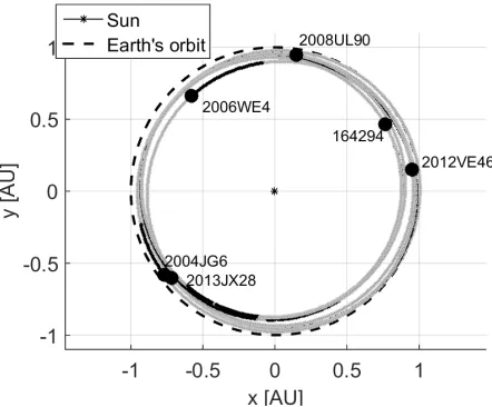
specific impulse considered is Isp = 3000 s. The spacecraft is injected into an interplanetary orbit which allows it to real-ize the first fly-by without switching on the engine. After the first fly-by the engine can be switched on to achieve the re-maining five fly-bys. The results of the optimised low-thrust transfers are reported in Table 4 and shown in Figure 2, where the thrust legs are in black and the coast legs are in grey.

Fig. 2. Trajectory for multiple fly-by of the Atira asteroids.

After the last fly-by the spacecraft is moved on an park-ing orbit with lower perihelion (0.725 AU). This allows the spacecraft to move to inner regions of the solar Systems to search for new NEAs. Two strategies to realise this trans-fer are considered. In the first one the low-thrust engine is used to alternate coast and thrust arc so as to reach the final parking orbit with the minimum∆V (Figure 3); in the sec-ond case the spacecraft is moved on an orbit that intersect the Earth’s one, so that a gravity assist with the Earth can be obtained (Figure 4). The transfer in Figure 3 is realized in 422 days and requires∆V = 1.8 km/s. The transfer real-ized through gravity-assist with the Earth takes 565 days but requires∆V = 1.31km/s.

3.2. Multiple Active Debris Removal Mission

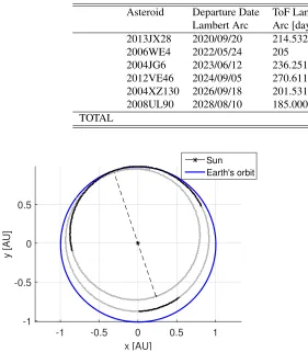
Table 2. Best solution obtained with six visited asteroids using AIDMAP with Lambert model.

Asteroid Departure Date ToF Lambert Arrival Date at ∆V [km/s] Lambert Arc Arc [days] Asteroid Node

2013JX28 2020/09/29 205 2021/04/22 0.87 2006WE4 2022/05/14 215 2022/12/15 0.86 2004JG6 2023/06/14 235 2024/02/04 0.61 2012VE46 2024/09/11 265 2025/06/03 0.36 2004XZ130 2026/09/15 205 2027/04/08 0.73 2008UL90 2028/07/31 195 2029/02/11 0.34

TOTAL 3.77

Table 3. Further optimisation of the best solution obtained with six visited asteroids using MP-AIDEA.

Asteroid Departure Date ToF Lambert Arrival Date at ∆V [km/s] Lambert Arc Arc [days] Asteroid Node

2013JX28 2020/09/20 214.5329 2021/04/22 0.95 2006WE4 2022/05/24 205 2022/12/15 0.69 2004JG6 2023/06/12 236.2514 2024/02/04 0.61 2012VE46 2024/09/05 270.6114 2025/06/03 0.34 2004XZ130 2026/09/18 201.5318 2027/04/08 0.72 2008UL90 2028/08/10 185.0003 2029/02/11 0.29

TOTAL 3.61

x [AU]

-1 -0.5 0 0.5 1

y [AU]

-1 -0.5 0 0.5

Sun Earth's orbit

Fig. 3. Trajectory for transfer to reduced perigee parking or-bit.

the active removal of five to ten large objects per year is re-quired to stabilize the population [38].

In this study a single servicing spacecraft equipped with electric engine is used for the de-orbiting of large satellites from the region between 800 and 1400 km in LEO. Two re-moval approaches are considered:

- Multi-target delivery of de-orbiting kits to perform a controlled re-entry;

x [AU]

-1 -0.5 0 0.5 1

y [AU]

-1 -0.8 -0.6 -0.4 -0.2 0 0.2 0.4 0.6 0.8 1

Earth-FlyBy Sun

Earth's orbit Final orbit

Fig. 4. Trajectory for transfer to reduced perigee parking orbit using a gravity assist with the Earth.

- Low-thrust fetch and de-orbit using the single towing spacecraft.

Table 4. Summary of leg-by-leg simulation results for optimal, six-leg, low-thrust trajectory.

Asteroid Time Engine m0[kg] mf [kg] ∆V [km/s]

On [days]

2013JX28 0 700 700

-2006WE4 129.05 700 673.45 1.12 2004JG6 152.57 673.45 642.07 1.37 2012VE46 41.77 642.07 633.47 0.40 2004XZ130 158.40 633.47 600.89 1.51 2008UL90 30.04 600.89 594.17 0.30

TOTAL 4.70

objects are then further selected based on two main criteria: the rate of the drift of the right ascension of the ascending node due to the second zonal harmonic of the gravity, J2, and the Criticality of Spacecraft Index (CSI), [39].

The change of right ascension, when realizing a transfer between two satellites, is realized by changing the semimajor axis of the servicing spacecraft and taking advantage of the dependence on the altitude of the natural rate of nodal regres-sion due to J2 [11]. Smaller inclination orbits are more favor-able for adjustment of right ascension realized by changing the semimajor axis [14], therefore the group of object with lower possible inclination is selected.

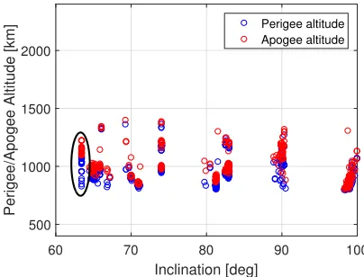
The targets are also selected based on their value of the Criticality of Spacecraft Index, which expresses the environ-mental criticality of objects in LEO taking into account the physical characteristics of a given object, its orbit and the en-vironment where it is located. After applying these selection criteria, a set of 25 objects are selected. The selected 25 ob-jects for this study are among the 100 most critical obob-jects in term of CSI [39]; the apogee and perigee altitude and in-clination of the selected targets (highlighted in the circle) are shown in Figure 5.

Inclination [deg]

60 70 80 90 100

Perigee/Apogee Altitude [km]

500 1000 1500 2000

Perigee altitude Apogee altitude

Fig. 5. Selected objects in LEO.

Once the database of objects is defined, the identification

of the optimal sequence of targets to be removed is realized using AIDMAP and a surrogate model of the cost (∆V) of the transfer of the low-thrust servicing spacecraft between ob-jects, obtained using FABLE.

For the computation of the cost associated to transfers between two satellites, the total transfer is divided into two phases [14]:

- in the first phase an optimisation problem is solved in order to adjuste,iandωin a given time of flight with the minimum propellant consumption;

- in the second phaseaandΩare adjusted, while keeping

iandeequal to the target’s ones and constrainingωto match the final argument of the perigee of the target orbit.

More details about the transfer model can be found in [14]. For the multi-target delivery of de-orbiting kits strat-egy, the sequence of transfer characterized by the lower total time of flight is reported in Table 5. Ten satellites, identified in Table 5 by their NORAD ID, can be serviced in less than one year. m0is the initial mass for the transfer and mf the mass at the end of the transfer. The 100 kg drop in mass after each transfer accounts for the attachment of the de-orbiting kit to the serviced satellite. T oFrepresents the time of flight required to realize the transfer andTwrepresents the waiting

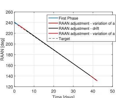
time on the orbit of the departure object required to obtain the orbital phasing with the arrival satellite. Figures 6 and 7 show the variation of orbital elements during the transfer from object 40342 to object 40338. These figures show how the use of the natural dynamics (J2) can be exploited to reach the desired value ofΩ.

Table 5. Sequence of removed satellite for servicing spacecraft delivering de-orbiting kits.

Departure Arrival ∆V T oF Tw,θ m0 mf

Object Object [km/s] [days] [hours] [kg] [kg] 1 39015 40343 0.0628 30.43 2.59 1900.00 1892.40 2 40343 40340 0.1128 65.75 1.78 1792.40 1779.55 3 40340 39016 0.0595 33.14 2.54 1679.55 1673.19 4 39016 40342 0.0429 29.73 2.70 1573.19 1568.89 5 40342 40338 0.0339 42.28 2.06 1468.89 1465.72 6 40338 40339 0.0013 7.05 1.78 1365.72 1365.60 7 40339 39011 0.1116 44.55 2.43 1265.60 1256.63 8 39011 39012 0.0035 14.19 2.07 1156.63 1156.37 9 39012 39013 0.0448 28.04 2.07 1056.37 1053.34

Total - - 0.4731 294.17 20.04 -

-Time [days]

0 10 20 30 40 50

Semimajor axis [km]

7440 7445 7450 7455 7460 7465 7470 7475

First Phase

RAAN adjustment - variation of a RAAN adjustment - drift RAAN adjustment - variation of a Target

Fig. 6. Variation ofaduring transfer from object 40342 to object 40338.

dispose of the 2000 kg serviced satellites and this results in an increased acceleration in the raising phase. The deorbiting is realized using continuous negative tangential acceleration while the orbit raising is performed with continuous positive tangential acceleration. The tools implemented in FABLE al-low to realise the deorbiting also by increasing the eccentric-ity of the orbit, applying a negative tangential thrust at apogee and a positive tangential thrust at perigee. In this case the re-entry conditions will be different from the ones obtained deorbiting with continuous tangential acceleration because of the increased eccentricity of the re-entry orbit (the fligth path angle at re-entry increases from≈0 to 1.5 deg). The variation of perigee and apogee altitude in this case is shown in Figure 9.

An application of the multi-fidelity optimisation of sur-rogate models described in Section 2.1 can be considered by looking at the first transfer between satellite deorbited by means of de-orbiting kits. As reported in Table 5 the transfer is from object 39015 to object 40343. A surrogate model

Time [days]

0 10 20 30 40 50

RAAN [deg]

120 140 160 180 200 220 240 260

First Phase

RAAN adjustment - variation of a RAAN adjustment - drift RAAN adjustment - variation of a Target

Fig. 7. Variation ofΩduring transfer from object 40342 to object 40338.

Table 6. Sequence of removed satellite for servicing satellite fetching non-operational satellite.

Departure Arrival ∆V T oF Tw,θ m0 mf

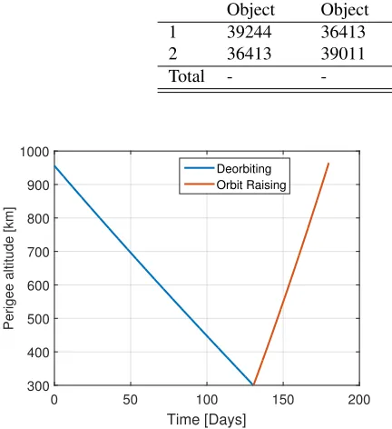
Object Object [km/s] [days] [hours] [kg] [kg] 1 39244 36413 1.1307 159.91 2.09 3000.00 890.11 2 36413 39011 0.9811 182.32 2.41 2890.11 802.79

Total - - 2.6118 373.23 4.5 -

-Time [Days]

0 50 100 150 200

Perigee altitude [km]

300 400 500 600 700 800 900 1000

Deorbiting Orbit Raising

Fig. 8. Variation of the perigee altitude for the servicing spacecraft during deorbit of object 36413 and orbit raising to the semimajor axis of target object 39011.

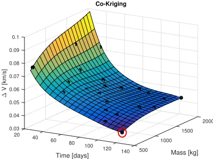
MP-AIDEA. The high-fidelity function is evaluated in the point of maximum expected improvement, the co-Kriging surrogate model is computed again and the process is re-peated. The representation of the expected improvement at the first step of the iterative procedure is shown in Figure 12.

The iteration stops after three runs, corresponding to three additional sampling in the most promising area (high time of flight, low spacecraft mass), when the expected improvement is lower than a pre-defined value. The Co-Kriging surrogate model at the end of the iterative process is shown in Figure 13. The minimum is correctly located atm = 600 kg and time of flight equal to 122 days.

4. CONCLUSION

In this paper CAMELOT, a toolbox for the design and op-timisation of multi-target low-thrust trajectories mission, has been presented. The three main components of CAMELOT, FABLE, MP-AIDEA and AIDMAP have been described. The toolbox has been applied to two case studies, the design of an interplanetary trajectory to visit the Atira asteroids and the de-sign of a mission to deorbit multiple non-cooperative objects from LEO. Results have shown that CAMELOT can solve different space problems in an efficient way while remaining easily adaptable to different applications.

Time [days]

0 50 100 150 200 250 300 350 400

Height [km]

0 200 400 600 800 1000 1200 1400

Perigee height Apogee height

Fig. 9. Variation of perigee and apogee altitude for re-entry with increase of eccentricity.

5. ACKNOWLEDGMENTS

This research was partially supported by Airbus Defence and Space. The authors would like to thank Mr. Stephen Kemble for his support and contribution.

6. REFERENCES

[1] S. N. Williams and V. Coverstone-Carroll, “Benefits of solar electric propulsion for the next generation of plan-etary exploration missions,” Journal of the Astronauti-cal Sciences, vol. 45, no. 2, pp. 143–159, 1997.

[2] C. G. Sauer and C. W. L Yen, “Planetary mission capa-bility of small low power solar electric propulsion sys-tems,”Acta Astronautica, vol. 35, pp. 625–634, 1995.

[3] J.T. Olympio and N. Frouvelle, “Space debris selection and optimal guidance for removal in the SSO with low-thrust propulsion,” Acta Astronautica, vol. 99, pp. 263– 275, jun 2014.

[4] M. Cerf, “Multiple space debris collecting mission. de-bris selection and trajectory optimization,” .

2000

1500

m [kg] 1000

500 150 100

ToF [days] 50 0 0.02 0.04 0.06 0.08 0.1

∆

V [km/s]

Fig. 10. Surrogate model of the cost of the transfer between objects 39015 and 40343.

2000

Mass [kg]

1500 1000 500 140

Co-Kriging

120 100

Time [days]

80 60 40 20 0.06

0.04 0.08

0.02

0 0.1

∆

V [km/s]

Fig. 11. Co-Kriging surrogate model of the cost of the trans-fer between objects 39015 and 40343.

[6] A. Ruggiero, P. Pergola, S. Marcuccio, and M. An-drenucci, “Low-thrust maneuvers for the efficient cor-rection of orbital elements,” in32nd International Elec-tric Propulsion Conference, 2011, pp. 1–13.

[7] T. N. Edelbaum, “Propulsion requirements for control-lable satellites,” ARS Journal, vol. 31, no. 8, pp. 1079– 1089, 1961.

[8] J. A. K´echichian, “Analytic representations of optimal low thrust transfer in circular orbits,”Spacecraft Trajec-tory Optimization, vol. 29, pp. 139, 2010.

[9] S. da Silva Fernandes, F. das Chagas Carvalho, and R. V. de Moraes, “Optimal low-thrust transfers between coplanar orbits with small eccentricities,” Computa-tional and Applied Mathematics, pp. 1–14, 2015.

[10] E. G. C. Burt, “On space manoeuvres with continuous

2000

Mass [kg] 1500

1000

500

Expected Improvement

140 120 100

Time [days] 80 60 40 ×10-3

20 1.5 2 2.5 3

0 0.5 1

EI [km/s]

Fig. 12. Expected improvement for the surrogate model of the cost of the transfer between objects 39015 and 40343.

2000

Mass [kg]

1500 1000 500 140

Co-Kriging

120 100

Time [days]

80 60 40 20 0.09 0.1

0.08

0.03 0.04 0.05 0.06 0.07

∆

V [km/s]

Fig. 13. Co-Kriging surrogate model at the last iteration of the maximization of the expected improvement.

thrust,” Planetary and Space Science, vol. 15, no. 1, pp. 103–122, 1967.

[11] J. E. Pollard, “Simplified analysis of low-thrust orbital maneuvers,” Tech. Rep., DTIC Document, 2000.

[12] A. E. Petropoulos, “Simple control laws for low-thrust orbit transfers,” 2003.

[13] F. Zuiani and M. Vasile, “Extended analytical formulas for the perturbed keplerian motion under a constant con-trol acceleration,” Celestial Mechanics and Dynamical Astronomy, vol. 121, no. 3, pp. 275–300, 2015.

[15] S. N. Lophaven, H. B. Nielsen, and J. Søndergaard, “Dace-a matlab kriging toolbox, version 2.0,” Tech. Rep., 2002.

[16] C. Ortega, A. Riccardi, M. Vasile, and C. Tardioli, “Smart-uq: Uncertainty quantification toolbox for gen-eralized intrusive and non intrusive polynomial algebra,” in6th ICATT, 2016.

[17] A. I. J. Forrester, A. S´obester, and A. J. Keane, “Multi-fidelity optimization via surrogate modelling,” in Pro-ceedings of the royal society of london a: mathematical, physical and engineering sciences. The Royal Society, 2007, vol. 463, pp. 3251–3269.

[18] D. J. J. Toal, “Some considerations regarding the use of multi-fidelity kriging in the construction of surrogate models,”Structural and Multidisciplinary Optimization, vol. 51, no. 6, pp. 1223–1245, 2015.

[19] I. Couckuyt, T. Dhaene, and P. Demeester, “oodace tool-box: a flexible object-oriented kriging implementation,” The Journal of Machine Learning Research, vol. 15, no. 1, pp. 3183–3186, 2014.

[20] D. R. Jones, “A taxonomy of global optimization meth-ods based on response surfaces,” Journal of global op-timization, vol. 21, no. 4, pp. 345–383, 2001.

[21] K. Price, R. M. Storn, and J. A. Lampinen, Differential evolution: a practical approach to global optimization, Springer Science & Business Media, 2006.

[22] M. Di Carlo, M. Vasile, and E. Minisci, “Multi-population inflationary differential evolution algorithm with adaptive local restart,” in 2015 IEEE Congress on Evolutionary Computation (CEC). IEEE, 2015, pp. 632–639.

[23] S. Das and P. N. Suganthan, “Differential evolution: a survey of the state-of-the-art,” IEEE Transactions on Evolutionary Computation, vol. 15, no. 1, pp. 4–31, 2011.

[24] R. G¨amperle, S. D. M¨uller, and P. Koumoutsakos, “A parameter study for differential evolution,” Advances in intelligent systems, fuzzy systems, evolutionary compu-tation, vol. 10, pp. 293–298, 2002.

[25] V. M. Becerra, D. R. Myatt, S. J. Nasuto, J. M. Bishop, and D. Izzo, “An efficient pruning technique for the global optimisation of multiple gravity assist trajecto-ries,”Acta Futura, vol. 2005, pp. 35, 2003.

[26] D. Novak and M. Vasile, “Incremental solution of lt-mga transfers transcribed with and advanced shaping approach,” in International Astronautical Congress, Prague, 27 September - 01 October 2010.

[27] M. Jepsen, B. Petersen, and S. Spoorendonk, “A branch-and-cut algorithm for the elementary shortest path prob-lem with a capacity constraint,” Department of Com-puter Science, . . ., , no. 08, 2008.

[28] S. Volker, “Formulations and branch-and-cut algorithms for the generalized vehicle routing problem,”Investment Management and Financial Innovations, vol. 5, no. 4, pp. 7–24, 2014.

[29] T. Nakagaki, H. Yamada, and ´A. T´oth, “Intelligence: Maze-solving by an amoeboid organism,” Nature, vol. 407, no. 6803, pp. 470–470, 2000.

[30] D. S. Hickey and L. A. Noriega, “Insights into informa-tion processing by the single cell slime mold physarum polycephalum,” inUKACC Control Conference, 2008, pp. 2–4.

[31] R. Kobayashi T. Saigusa T. Nakagaki A. Tero, K. Yu-miki, “Flow-network adaptation in physarum amoebae,” Theory in Biosciences, vol. 127, no. 2, pp. 98–94, 2008.

[32] J. M. Romero Martin, L. Masi, M. Vasile, E. Minisci, R. Epenoy, V. Martinot, and J. Fontdecaba Baig, “In-cremental planning of multi-gravity assist trajectories,” in65st International Astronautical Congress, IAC 2014, 2014, pp. Paper–IAC.

[33] L. Masi and M. Vasile, “A multidirectional physarum solver for the automated design of space trajectories,” July 6-11, 2014.

[34] M. Di Carlo, N. Ortiz G´omez, J. M. Romero Martin, C. Tardioli, F. Gachet, K. Kumar, and M. Vasile, “Opti-mized low-thrust mission to the atira asteroids,” in25th AAS/AIAA Space Flight Mechanics Meeting, 2015, pp. AAS15–299.

[35] S. Kemble,Interplanetary mission analysis and design, Springer Science & Business Media, 2006.

[36] D. J. Kessler, N. L. Johnson, J.C. Liou, and M. Matney, “The kessler syndrome: implications to future space op-erations,” Advances in the Astronautical Sciences, vol. 137, no. 8, pp. 2010, 2010.

[37] Inter-Agency Space Debris Coordination Committee et al., IADC space debris mitigation guidelines, Inter-Agency Space Debris Coordination Committee, 2002.

[38] J-C Liou and Nicholas L Johnson, “Instability of the present leo satellite populations,” Advances in Space Research, vol. 41, no. 7, pp. 1046–1053, 2008.