Forschungsinstitut zur Zukunft der Arbeit Institute for the Study
DISCUSSION PAPER SERIES
The Impact of Micro-Credit on Employment:
Evidence from Bangladesh and Pakistan
IZA DP No. 10046
July 2016 Azhar Kahn
The Impact of Micro-Credit on Employment:
Evidence from Bangladesh and Pakistan
Azhar Kahn
University of StrathclydeTwyeafur Rahman
University of StrathclydeRobert E. Wright
University of Strathclydeand IZA
Discussion Paper No. 10046
July 2016
IZA P.O. Box 7240
53072 Bonn Germany Phone: +49-228-3894-0 Fax: +49-228-3894-180
E-mail: iza@iza.org
Any opinions expressed here are those of the author(s) and not those of IZA. Research published in this series may include views on policy, but the institute itself takes no institutional policy positions. The IZA research network is committed to the IZA Guiding Principles of Research Integrity.
IZA Discussion Paper No. 10046 July 2016
ABSTRACT
The Impact of Micro-Credit on Employment:
Evidence from Bangladesh and Pakistan
This paper examines the impact of micro-credit on employment. Household-level data was collected, following a quasi-experimental design, in Bangladesh and Pakistan. Three borrower groups are compared: Current borrowers; Pipeline borrowers and Non-borrowers. Pipeline borrowers are included to control for self-selection effects. It is argued that micro-credit causes a substitution of employment away from employment-for-pay to self-employment. Therefore, the effect on total employment is ambiguous. OLS and fixed effects regression are used to examine separately self-employment and employment-for-pay between three groups of borrowers. For Pakistan, there is no evidence that micro-credit effects employment. However, for Bangladesh, there is robust evidence consistent with this hypothesis.
JEL Classification: G21, J22, I39
Keywords: micro-credit, poverty, self-employment
Corresponding author:
Robert E. Wright
Department of Economics Sir William Duncan Building University of Strathclyde 130 Rottenrow
Glasgow, G4 0GE United Kingdom
The Impact of Micro-credit on Employment: Evidence from Bangladesh and Pakistan
1. Introduction
There is considerable interest in the impact of micro-credit on poverty in low-income
countries. There is a growing belief amongst politicians and policy-makers that micro-credit is
a major poverty-reduction tool in such countries. However, despite the increasing popularity
of micro-credit, the results of empirical studies of its poverty-reducing impacts are at best
mixed. For example, Duvendack et al. (2011, p. 4), after a thorough review of a large number
of empirical studies, conclude: “… almost all impact evaluations of microfinance suffer from
weak methodologies and inadequate data… thus the reliability of impact estimates are
adversely affected. This can lead to misconceptions about the actual effects of a microfinance
programme”. Since more money for micro-credit, means less money for other poverty-reducing
interventions, it is critical to establish whether it does result in a sustained reduction in poverty.
There are various mechanisms by which micro-credit can impact on poverty. One
argument is that micro-credit increases employment. More specifically, micro-credit loans are
used to purchase capital, and once this capital in combined with available labour, there is an
increase in employment. Since employment is perhaps the best predictor of poverty, any policy
that increases employment, is potentially important in term of poverty reduction. However, we
believe this view is a serious over-simplification. It is our view that in order to understand this
relationship it is necessary to distinguish between the types of work being carried out. The key
distinction for us is between “employment-for-pay” and “self-employment”. Our hypothesis
is that micro-credit increases self-employment but decreases employment-for-pay. That is,
micro-credit leads to a substitution away from employment-for-pay to self-employment, with
self-employment are sufficiently above those for employment-for-pay, then the employment
impact of micro-credit could lead to lower poverty, even with no increase in overall
employment. If this is the case, then it is not surprising that empirical studies that have not
distinguished between these types of employment have very mixed results (see for example,
Al-Mamun, Wahab and Malarvizhi, 2011; Angelucci, Karlan and Zinman, 2015; Attanasio et
al., 2015; Augsburg et al., 2015; Garnani, 2007; Karlan and Zinman, 2011; Lensink and Pham,
2011; Khan, 1999; Khandker, Samad and Khan, 1998; McKernan, 2002;
Panjaitan-Drioadisuryo and Gould, 1999; and Pitt, 2000).
In order to explore this hypothesis empirically, this paper examines the relationship
between micro-credit and employment at the household-level in Bangladesh and Pakistan with
micro-level data collected following a quasi-experimental design. The remainder of the paper
is organised as follows. Section 2 presents the methodology and data. OLS and fixed effects
regression are used to examine separately self-employment and employment-for-pay between
three groups of borrowers. The estimates are given in Section 3. In Pakistan there is little
evidence consistent with the view that micro-credit causes a substitution away from
employment-for-pay to self-employment. However, in Bangladesh, there is robust evidence
consistent with this hypothesis. Concluding Comments follow in Section 4.
2. Methodology
The statistical analysis presented in this section uses survey data collected in
Bangladesh and Pakistan based on a “quasi-experimental” design (see Dinardo, 2008; Meyer,
1995; Todd, 2008). The design consists of three groups of households: (1) Current Borrowers;
(2) Non-borrowers and (3) Pipeline borrowers. “Current Borrowers” are households that at
time of interview, were in receipt of a micro-credit loan. “Non-borrowers” are households that
time of interview. Since these non-borrowers have never had a micro-credit loan, then there
can be no effect of micro-credit. If current borrowers are not a “self-selected” group, then a
comparison of current borrowers with non-borrowers would form the basis of a meaningful
comparison of the impact of micro-credit on employment.
There is however considerable concern that self-selection is a problem in the evaluation
of micro-credit. Households that apply for a micro-credit loan may be very different in terms
of both observable and non-observable characteristics that underpin the decision to apply for a
loan (see Tedeschi, 2007). Put differently, it is unlikely that borrowers are a random subset of
all potential borrowers. It is possible to control statistically for certain observable
characteristics through (for example) multiple-regression. However, non-observable
characteristics are unmeasured, and therefore cannot be controlled for in the same way. It is
possible to control for self-selection by comparing current borrowers and non-borrowers to
so-called “Pipeline borrowers”. Pipeline borrowers are households that have successfully applied
for a micro-credit loan but at the time of interview had not received the money. Since they have
applied for a loan they are similar to current borrowers in unobserved characteristics. Put
differently, it is difficult to imagine why they would be different in unobserved characteristics
(especially after controlling for observed differences). Pipeline borrowers have never held a
micro-credit loan and have not yet received the money for what will become their current loan.
Therefore, for this group of borrowers there can be no micro-credit effects caused by
spending/investing since they do not have the money in hand to do so (see Coleman, 1999
2006; Chowdhury, Ghosh and Wright; 2005, Karlan, 2001; Khan and Wright, 2015).
A comparison of current borrowers, pipeline borrowers and non-borrowers can be used
to more convincingly estimate the impact of micro-credit on employment. Any difference
between non-borrowers and pipeline borrowers can be attributed to self-selection (and not to
attributed to micro-credit. However, this assumes that other factors that impact on employment
are “held constant”, since micro-credit is not the only possible factor affecting employment.
Multiple regression can be used to control for measured factors, such as age, education and
household size. In addition, it is likely the case that geographic location has an effect on
employment. More specifically, in countries such as Bangladesh and Pakistan, there is
considerable geographic variation is the quantity and quality of arable land. Given agriculture
is the main form of employment in both of these countries, it is not difficult to believe that
arable land is a key determinant of employment patterns. It is difficult to measure this
variability directly. However, fixed effects can be used to proxy this potentially important
geographical variation. If micro-credit does have an impact on employment, you would expect
such effects to be largely unaffected by the inclusion of geographically-defined fixed effects.
Further details of the statistical model are discussed below.
2.1. Data
The data for Pakistan was collected in the period December, 2008 to February, 2009.
Face-to-face interviewing was used. The sampling frame used to draw the sample of current
borrowers and pipeline borrower is based on three microcredit lending institutions: (1)
Khushhali Bank Limited; (2) National and Rural Support Programme; and (3) Akhuwat. The
authors believe that these three institutions represent well the micro-credit sector in Pakistan.
The total sample size is 468 households (see Table 1).This is the same data used in Khan and
Wright (2015), and we refer the reader to this study for further detail.
The data for Bangladesh was collected in the period June. 2014 to September, 2014.
Face-to-face interviewing was used. The sampling frame was provided by the Association for
Social Advancement, more commonly known as “ASA”. Established in 1978, ASA is the
Bank in Bangladesh. With nearly 3,000 branches, the authors believe that the scale of ASA’s
micro-credit activities makes it representatives of the sector as a whole. The total sample size
is 1,522 households (see Table 1). This is the same data used by Rahman (2016).
2.2. Statistical Model
The statistical model is of the form:
ln(Emp)ij = α0 + α1Currentij + α2Pipelineij + α3ln(Ageij) + α4ln(Schoolij) + α5ln(nChildFij) +
α6ln(nChildMij)+ α7ln(nAdultFij) + α8ln(nAdultMij) + α9ln(nOlderFij) +
α10ln(nOlderMij) + θj + µi
where “Emp” is the number of individuals in household “i” in region “j” who are employed.
“Current” is a dummy variable coded “1” if the household is a current borrower and coded “0”
if not. “Pipeline” is a dummy variable coded “1” if the household is a pipeline borrowers and
coded “0” if not. The excluded category is non-borrower. “Age” is the age of the household
head. “School” is the number of years of education of the household head. “nChildF” and
“nChildM” are the number of female and male children in the household. “nAdultM” and
“nAdultF” are the number of female and male adults (less than age 65) on the
household.“nOlderM” and “nOlderF” are the number of email and male elderly adults (age 65
and older) in the household. “θ”is a regional-level fixed effect (discussed below) and “µ” is a
random error term. Since all the variables are expressed in natural logarithms (except “Current”
and “Pipeline”), the parameters can be interpreted as elasticities.
The inclusion of “Age” and “School” are intended to capture differences in the head of
the household. Since household heads are traditionally the main decision-makers in
socioeconomic differences that may affect decisions relating to the employment of household
members. The sex-specific number of children, number of adults and number of elderly adults
is intended to represent the number of potential workers in the households. These variables
sum to total household size. Holding other factors constant, you would expect larger
households to have a larger number of household members employed.
θj are regional-level fixed effects. Fixed effects control for persistent differences across
regions that impact on employment. In Pakistan, the fixed effects are based on 30 “Union
Council” areas. A union council is an elected local government for a small group of villages in
close geographical proximity. In Bangladesh, the fixed effects are based on 54 “Thana” areas.
Traditionally a Thana was an area controlled by a police station. If micro-credit does have an
impact on employment, then you would expect to find a similar set of parameters for key
variables in regression models with and without fixed effects. That is, the estimates are robust
to the inclusion of variables that capture persistent differences across regions. If the opposite
is the case, then one possible conclusions is that it is regional differences—and not
micro-credit—that is important in explaining differences in employment across households. In other
words, if micro-credit is a true determinant of differences in employment across households,
you would not expect the inclusion of geographically-defined fixed effect to have impact on
the estimates.
The numbers employed in the household, “Emp”, is measured in three ways. The first
is the total number of household members employed, consisting of both those
for-pay and those self-employed. The second is only the number of household members
employed-for-pay. The third is the number of household members who are self-employed. Estimating
regression models separately for these three measures of household employment will provide
Remembering that the excluded category is “Non-borrowers”, the marginal difference in
percentage terms of being a current borrower relative to a non-borrower is:
A = Effect(CB:NB) = [exp(α1)-1] x 100.
In turn, the marginal effect of being a pipeline borrower relative to a non-borrower is:
B = Effect(PB:NB) = [exp(α2)-1] x 100.
As discussed above, the latter difference can be attributed to self-selection effects and not to
micro-credit. Therefore the effect of micro-credit on employment, purged of self-selection
effects, is the difference between current borrowers effect and pipeline borrowers:
Difference = A - B = Effect(CB:NB) - Effect(PB:NB).
3. Results
Table 1 reports the means and standard deviations for the three employment variables
broken down by borrower groups. The upper panel of the table is for Pakistan while the lower
panel is for Bangladesh. Also shown in this table is an F-test that provides a statistical test of
the differences across the three borrower groups. It is interesting to note that for both countries
the F-test suggests that there is no statistically significant difference across the groups when
those employed-for-pay and those self-employed are lumped together (denoted “Both” in the
table).
<<<< Table 1 About Here >>>>
The situation is, however, quite different when the two types of employment are
considered separately. In Pakistan, the number of self-employed is higher for current borrowers
and pipeline borrowers than for non-borrowers, and this difference is statistically significant at
below the 1% level. Likewise, the number of employed-for-pay is lower for current borrowers
and pipeline borrowers than for non-borrowers, although this difference is only statistically
it appears that self-employment compared to employment-for-pay is higher for current
borrowers compared to non-borrowers. However, the same is the case for pipeline borrowers
compared to non-borrowers. This finding is suggestive of self-selection given that pipe-line
borrowers have not received the loan and the money is not yet available to enhance
self-employment. It is likely that households that apply for micro-credit loans have above average
levels of self-employment and below average level of employment-for-pay prior to applying.
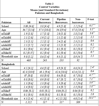
The across borrower groups differences shown in Table 1 do not control for other
factors that potentially impact on employment. Table 2 reports the means and standard
deviations for the control variables included in the regression models. The table also reports
F-test that F-tests for difference in these variables across the three borrower groups. It is clear from
this table that there are differences across these groups but that the pattern is not consistent
between the two countries. For example, in Pakistan the level of schooling of household heads
is much higher for current borrowers compared to non-borrowers. However, it is even higher
for pipe-line borrowers. In Bangladesh, the opposite is observed—the level of schooling of
household heads is lower for current borrowers compared to non-borrowers. Like in Pakistan,
the level of school of household heads is highest for pipeline borrowers. There are also a
significant differences in the age of household heads in Pakistan across the groups but this is
not the case in Bangladesh. There are also differences in the age and sex mix of household of
members but the pattern is not the same between the two countries. This suggests that the
differences in the control variables across the three groups summarised in Table 2 does not
provide a “neat” explanation of the differences in the employment variables summarised in
Table 1.
<<<< Table 2 About Here >>>>
Table 3 reports the estimates of the regression models where the dependent variable is
numbers self-employed added together). Columns (1) and (2) are OLS estimates and Columns
(3) and (4) are fixed effect estimates. Turning first to the OLS estimates, in both countries, the
pipeline borrowers dummy is not statistically significant. However, the current borrower
variables is statistically significant, at the 5% level in Pakistan and at the 10% level in
Bangladesh, with a positive sign. This suggests that total employment is higher for current
borrowers compared to non-borrower households. In addition, there is no difference in total
employment between pipeline borrowers and non-borrowers. The point estimates indicate that
total employment is about 10.6% higher in Pakistan, and 6.4% higher in Bangladesh, compared
to non-borrowers. However, when fixed effects are added, this difference disappears for
Pakistan [see Column (3)], suggesting that there are no statistically significant difference across
the three borrower groups. However, for Bangladesh when fixed effect are added, the
difference remains statistically significant, with total employment being higher for current
borrowers compared to pipeline borrowers and non-borrowers [see Column (4)].
<<<< Table 3 About Here >>>>
The estimates in Table 3 suggest a positive relationship between the age of the
household head and numbers employed. However, this relationship is only statically significant
in Bangladesh. Somewhat surprisingly, there is a negative relationship between the schooling
of the household head and number employed. Again this relationship is only statistically
significant in Bangladesh. It is important to note that in both countries there is a positive
relationship between the number of both female and male “adult” household members and
numbers employed. The same is the case for “older” male household members but not for
“older” female household members. However, the estimates are quite mixed for the number of
female and male children in the household. One must be careful with the interpretation of these
child variables as they potentially capture information about the prevalence of child labour (as
Table 4 reports the estimates of the regression models where the dependent variable is
the total number of household members who are employed-for pay. The layout is the same as
Table 3. These estimates are best viewed relative to the estimates of the regression models
where the dependent variable is the total number of household members who are
self-employed. These estimates are shown in Table 5. It is not an exaggeration to conclude that the
borrower group variables in Table 4 are the “mirror image” of the estimates in Table 5. More
specifically, the OLS estimates shown in Table 4 [Columns (1) and (2)] suggest that in both
countries the numbers employed-for-pay is lower for current borrowers compared to
non-borrowers. However, the OLS estimates shown in Table 5 suggest that in both countries the
numbers self-employed is higher for current borrowers compared to non-borrowers.
<<<< Tables 4 and 5 About Here >>>>
Focussing on the OLS estimates only, one could conclude that micro-credit exerts a
positive impact on self-employment and a negative impact on employment-for-pay. These
estimates are also indicative of micro-credit being associated with a substitution away from
employment-for-pay to self-employment. However, for Pakistan when fixed effects are added
none of the borrower group variables are statistically significant. However, this is not the case
for Bangladesh. When fixed effects are added, employment-for-pay is lower and
self-employment is higher for current borrowers compared to non-borrowers. In addition, for
Bangladesh the estimates for pipe-line borrower suggest that there is little difference in the
numbers employed-for-pay and numbers self-employed between pipeline borrowers and
non-borrowers.
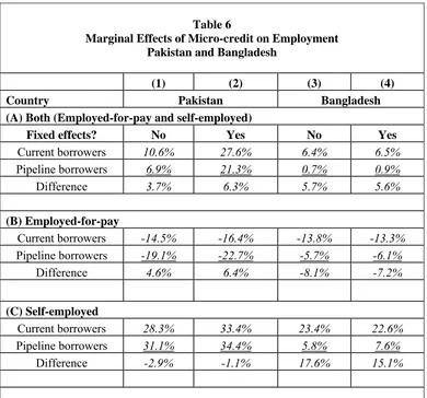
Table 6 gives the marginal effects for each of the borrower groups based the regression
estimates given in Tables (3), (4) and (5). As discussed above, the difference in the marginal
effects between pipeline borrowers and non-borrowers can be interpreted as a selection effect,
the marginal effects between current borrowers and pipeline borrowers is purged of selection
effects, and as a consequence can be interpreted as micro-credit effect. Therefore, this key
estimate in Table 6 is shown in the rows labelled “Difference”.
<<<< Table 6 About Here >>>>
Turning first to Panel (A) in Table 6, the main finding is that the estimates of the impact
of micro-credit on total employment are small. For Pakistan, the “Difference” estimates based
on OLS regression is 3.7% and slightly higher at 6.3% based on fixed effects regression. For
Bangladesh, the “Difference” estimates are not too different from those for Pakistan: 5.7%
based on OLS regression and 5.6% based on fixed effects regression. It is interesting to note
that most of the difference in numbers employed between current borrowers and non-borrowers
in Pakistan can be attributed to selection effects and not to micro-credit. The marginal effect
for current borrowers/non-borrowers is 10.6% based on OLS regression and 27.6% based on
fixed effects regression. The marginal effect for pipeline borrowers/non-borrowers is 6.9%
based on OLS regression and 21.3% based on fixed effects regression. Based on OLS
regression, about 65% of the difference between current borrowers is due to selection effects
(i.e. 6.9%/10.6% is a difference of 65.1%). Based on fixed effects regression, the difference is
nearly 80% (i.e. 21.3%/27.6% is a difference of 77.2%).
On the other hand, in Bangladesh most of the difference in numbers employed between
current borrowers and non-borrowers cannot be attributed to selection effects. The marginal
effect for current borrowers/non-borrowers is 6.4% based on OLS regression and 6.5% based
on fixed effects regression. The marginal effect for pipeline borrowers/non-borrowers is 0.7%
based on OLS regression and 0.9% based on fixed effects regression. Based on OLS regression,
about 10%of the difference between current borrowers is due to selection effects (i.e.
0.7%/6.4% is a difference of 10.9%). Based on fixed effects regression, the difference is nearer
to the regression method used—the estimates are very similar for both OLS and fixed effects
regression. Given this robustness, coupled with the small selection effects, there is a stronger
case to attribute the difference in total number employed between current borrowers and
non-borrowers to micro-credit in Bangladesh.
Panel (B) of Table 6 gives the marginal effects based on the regression models where
the dependent variable is the numbers employed-for-pay. Turning first to the estimates for
Pakistan, there is little evidence that micro-credit impacts on the numbers employed-for-pay.
The marginal effect for current borrowers/non-borrowers is -14.5% based on OLS regression
and -16.4% based on fixed effects regression. That is, the numbers employed-for-pay is lower
for current borrowers and for non-borrowers. However, the marginal effect for pipeline
borrowers/non-borrowers is -19.1% based on OLS regression and -22.7% based on fixed
effects regression. In other words, the marginal effect for pipeline borrowers/non-borrowers is
larger in absolute value than the marginal effect for pipe-line borrowers. This results in a
“Difference” estimate of +4.6% based on OLS regression and +6.4% based on fixed effects
regression. Again this supports the finding that most of the difference in employment between
current borrowers and non-borrowers is due to selection effects.
The marginal effects shown for Bangladesh in Table 6 for employed-for-pay [Panel
(B)] suggest that the numbers employed-for-pay is lower for current-borrowers compared to
non-borrowers. The marginal effect for current borrowers/non-borrowers is -13.8% based on
OLS regression and -13.3% based on fixed effects regression. That is, the numbers
employed-for-pay is lower for current borrowers and for non-borrowers. However, the marginal effect for
pipeline borrowers/non-borrowers is -5.7% based on OLS regression and -6.1% based on fixed
effects regression. This results in a “Difference” estimate of -8.1% based on OLS regression
and -7.2% based on fixed effects regression. The OLS estimates suggests that around 40% of
be attributed to selection effects (i.e. the difference -5.7%/-13.8% as a percentage is 41.3%)
and around 60% can be attributed to micro-credit (i.e. the difference -8.1%/-13.8% as a
percentage is 58.7%). The fixed effects estimates suggests that around 45% of difference in the
numbers employed-for pay between current borrowers and non-borrowers can be attributed to
selection effects (i.e. the difference -6.1%/-13.3% as a percentage is 45.9%) and around 55%
can be attributed to micro-credit (i.e. the difference -87.2%/-13.3% as a percentage is 54.1%).
Unlike what was found for Pakistan, around half the difference between current borrowers and
non-borrowers can be attributed to selection effects while the other half can be attributed to
micro-credit.
Panel (C) of Table 6 shows the marginal effects based on the regression models where
the dependent variable is the numbers self-employed. For both countries, the marginal effects
for current borrowers/non-borrowers is positive and quite large in magnitude. Turning first to
the estimates for Pakistan, the marginal effect for current borrowers/non-borrowers is 28.3%
based on OLS regression and 33.4% based on fixed effects regression. Again it is the case that
most of this difference can be attributed to selection effects. In fact, the marginal effects for
pipeline borrowers/non-borrowers are large. More specifically, 31.1% is based on OLS
regression and 34.4% is based on fixed effects regression. Given these large magnitudes, it is
not surprising to find that the “Difference” estimates are negative and very small in magnitude.
This suggests that most, if not all, of the difference in the numbers of self-employed between
current borrowers and non-borrowers is due to selection effects.
The situation is quite different for Bangladesh. The marginal effect for current
borrowers/non-borrowers is 23.4% based on OLS regression and 22.6% based on fixed effects
regression. The marginal effects for pipeline borrowers/non-borrowers are sizeable. More
specifically, 5.8% based on OLS regression and 7.6% based on fixed effects regression. This
fixed effects regression. The OLS estimates suggests that around 25% of the difference in the
numbers self-employed between current borrowers and non-borrowers can be attributed to
selection effects (i.e. the difference 5.8%/23.4% as a percentage is 24.8%) and around 60% can
be attributed to micro-credit (i.e. the difference 17.6%/23.4% as a percentage is 75.2%). The
fixed effects estimates suggests that around 35% of the difference in the numbers
employed-for pay between current borrowers and non-borrowers can be attributed to selection effects (i.e.
the difference 7.6%/22.6% as a percentage is 33.6%) and around 55% can be attributed to
micro-credit (i.e. the difference 15.0%/22.6% as a percentage is 66.4%). Again unlike what
was found for Pakistan, around 25%-35% of the difference between current borrowers and
non-borrowers can be attributed to selection effects while the between 55%-65% can be attributed
to micro-credit.
4. Concluding Comments
This paper examined the relationship between micro-credit and employment.
Proponents of micro-credit argue that micro-credit is poverty-reducing in the sense that it leads
to more household members being employed. With more household members working, more
income is generated, which reduces the risk of poverty. Our view is that this mechanism is at
best misleading. We test the hypothesis that micro-credit may cause a substitution of
employment away from employment-for-pay to self-employment. If this is the case, then
impact of micro-credit on total employment is ambiguous.
This hypothesis was tested with household-level survey data for Pakistan and
Bangladesh based on a quasi-experimental design. This data was used to test for differences in
self-employment across three groups of borrowers: Current borrowers, Pipeline borrowers and
Non-borrowers. The inclusion of Pipeline borrower is a way of potentially controlling for
borrowers and non-borrowers likely exaggerates the impact of micro-credit on employment.
The models were estimated by OLS and fixed effects regression. The inclusion of fixed effects
based on geographic regions (i.e. Union Councils and Thanas) provide an additional control
for unmeasured differences in employment opportunities based on the area where the
household is located.
The findings were mixed in the sense that the findings for Pakistan and Bangladesh
were quite different. For Pakistan there no robust statistical evidence suggesting that
micro-credit effects increasing employment were found. Selection effects were found to be large. In
addition, the estimates varied considerably depending on whether OLS or fixed effect
regression was used. This suggests that regional-specific factors, such as the quantity and
quality of arable land, are likely important in the observed employment differences across
households. While the Pakistan analysis is disappointing in terms of the main hypothesis, there
is robust statistical evidence in support of it in Bangladesh. However, it is important to note
that sizeable selection effects are also found but these effects are much smaller than what was
found for Pakistan. In addition, the estimates are very similar for both OLS and fixed effects
regression. This suggest that regional-specific factors are of less importance. For Bangladesh,
based on fixed effects regression, micro-credit is associated with a 23% higher level of
self-employment; a 7.2% lower level of employment-for-pay; and a 5.6% higher level of total
employment [See Column (4) in Table 6].
It must be remembered that the data used in the analysis was based on the same
quasi-experimental design. It is therefore of concern that the findings for the two countries are not
similar. However, the overall analysis does suggests that it is potentially important to
distinguish between different types of employment. One benefit of doing this is that it helps
understand the mechanisms by which micro-credit impacts on poverty. Therefore surveys
members the type of work they are doing. We expect that in reality a share of adults in poor
Pakistani and Bangladeshi households combined self-employment with employment-for-pay
but only report to interviewers their main type of employment.
As was mentioned above, the age and sex structure of the household is important to the
understanding of employment differences across households. At the simplest level, this
suggests (not surprisingly) that large households have more household members employed.
The number of adult female and male household and the number of adult older male household
members is especially important in this respect. It is important to note that the number of male
and female children in the household is not important. In most of the regression models
summarised in Tables (3), (4) and (5), the number of children in the household variables were
not statistically significant. In the few number of cases where this was not the case, the sign of
relationship was negative. This provides some indirect evidence that micro-credit does not lead
to higher levels of child employment. However, to fully appreciate the effect that micro-credit
has on employment, analysis must be carried that not examines for employment-for-pay and
self-employment separately by age and sex.
References
Al-Mamun, A., S.A. Wahab and C.A. Malarvizhi (2011), “Examining the Effect of Microcredit
on Employment in Peninsular Malaysia”, Journal of Sustainable Development, vol. 4,
no. 2, pp. 174-183
Angelucci M., D. Karlan, and J. Zinman, (2015), “Microcredit Impacts: Evidence from a
Randomized Microcredit Program Placement Experiment by Compartamos Banco”,
American Economic Journal: Applied Economics, vol. 7, no. 1, pp. 151–182
Attanasio, O., B. Augsburg, R. De Haas, E. Fitzsimons and H. Harmgart, (2015), “The Impacts
of Microfinance: Evidence from Joint-Liability Lending in Mongolia”, American
Economic Journal: Applied Economics, vol. 7, no. 1, pp. 90–122
Augsburg, B., R. De Haas, H. Harmgart and C. Meghir, (2015), “The Impacts of Microcredit:
Evidence from Bosnia and Herzegovina”, American Economic Journal: Applied
Economics, vol. 7, no. 1, pp.183–203
Coleman, B.E., (1999), “The Impact of Group Lending in Northeast Thailand”, Journal of
Development Economics, vol. 60, no. 1, pp. 105-141
Coleman, B.E., (2006), “Microfinance in Northeast Thailand: Who Benefits and How Much?”,
World Development, vol. 34, no. 9, pp. 1612-1638
Chowdhury. M.J.A., D. Ghosh and R.E. Wright, (2005), “The Impact of Micro-credit on
Poverty: Evidence form Bangladesh”, Progress in Development Studies, vol. 5, no. 2,
pp. 298-309
Dinardo, J., (2008), "Natural Experiments and Quasi-natural Experiments", New Palgrave
Duvendack, M., R. Palmer-Jones, J.G. Copestake, L. Hooper, Y. Loke and N. Rao, (2011),
What is the Evidence of the Impact of Microfinance on the Well-being of Poor People?
London. Institute of Education, University of London
Garnani, A.G., (2007), Employment, Not Microcredit, is the Solution, Working paper no. 1065,
Ann Arbor, Michigan, Ross School of Business, University of Michigan
Karlan, D. and J. Zinman, (2011), “Microcredit in Theory and Practice: Using Randomized
Credit Scoring for Impact Evaluation”, Science, vol. 332, no. 6035, pp. 1278-1284
Lensink, R and T.T.T. Pham, (2011), “The Impact of Microcredit on Self-Employment Profits
in Vietnam”, Economics of Transition, vol. 20, no 1, pp. 73-111
Karlan, D., (2001), “Microfinance Impact Assessments: The Perils of Using News Members
as a Control Group”, Journal of Microfinance, vol. 3, no. 2, pp 75-85
Khan, M.R., (1999), “Microfinance, Wage Employment and Housework: A Gender Analysis,
Development in Practice, vol. 9, no. 4, pp. 424-436,
Khan, M.A. and R.E. Wright, (2015), “Micro-credit, Entrepreneurship and Household
Outcomes”, Journal of Social Business, vol. 5, no. 2/3, pp. 3-30
Khandker, S.R., H.A. Samad and Z.H. Khan (1998), “Income and Employment Effects of
Micro‐credit Programmes: Village‐level evidence from Bangladesh”, Journal of
Development Studies, vol. 35. no. 2, pp. 96-124
McKernan, S.M., (2002), “The Impact of Microcredit Programs on Self-Employment Profits:
Do Noncredit Program Aspects Matter?”, Review of Economics and Statistics, vol. 84,
no. 1, pp. 93-115
Meyer, B.D., (1995), “Quasi & Natural Experiments in Economics”, Journal of Business and
Panjaitan-Drioadisuryo, R.D.M. and K. Gould, (1999), “Gender, Self-employment and
Microcredit programs: An Indonesian Case Study” Quarterly Review of Economics and
Finance, vol. 39, no 5, pp. 769-779
Pitt, M.M., (2000), “The Effect of Non-agricultural Self- employment Credit on Contractual
Relations and Employment in Agriculture: The Case of Microcredit Programmes in
Bangladesh”, Bangladesh Development Studies, vol. 26, no. 2/3, pp. 15-48
Rahman. M.T, (2016), The Role of Micro-credit Programmes in Alleviating Poverty in
Bangladesh. PhD Dissertation in Economics, University of Strathclyde, Glasgow
Tedeschi, G.A., (2007), “Overcoming Selection Bias in Microcredit Impact Assessments”,
Journal of Development Studies, vol. 44, no. 32, 504-518
Todd, P.E., (2008), “Evaluating Social Programs with Endogenous Program Placement and
Selection of the Treated”, In: Handbook of Development Economics, edited by T.P.
Table 1
Numbers Employed by Borrower Group Means [and Standard Deviations]
Pakistan and Bangladesh
Pakistan All Current Borrowers
Pipeline Borrowers
Non-borrowers
F-test
(a) Self-employed 2.2 [1.6] 2.3 [1.5] 2.4 [1.7] 1.6 [1.3] 4.9***
(b) Employed-for-pay 0.6 [1.0] 0.6 [0.9] 0.5 [0.8] 0.9 [1.4] 3.8*
Both (a) + (b) 2.8 [1.7] 2.8 [1.6] 2.9 [1.9] 2.5 [1.5] 0.9
N 468 243 133 92
Bangladesh
(a) Self-employed 0.6 [0.7] 0.7 [0.8] 0.6 [0.7] 0.5 [0.7] 12.1***
(b) Employed-for-pay 0.9 [0.8] 0.7 [0.8] 0.9 [0.9] 0.9 [0.8] 6.6***
Both (a) +(b) 1.6 [0.8] 1.4 [0.8] 1.5 [0.8] 1.4 [0.7] 0.9
N 1,522 535 507 536
Table 2 Control Variables
Means [and Standard Deviations] Pakistan and Bangladesh
Pakistan All Current Borrowers
Pipeline Borrowers
Non-borrowers
F-test
School 3.80 [4.6] 3.8 [4.4] 4.9 [5.0] 2.2 [3.4] 6.1***
Age 36.7 [11.0] 37.3 [10.8] 34.1[9.4] 37.8 [13.6] 3.5**
nChildF 1.9 [1.8] 1.7 [1.8] 2.0 [1.8] 1.8 [1.6] 3.6**
nChildM 2.1 [2.0] 1.9 [2.1] 2.1 [2.0] 2.2 [1.9] 1.5
nAdultF 2.3 [1.5] 2.2 [1.5] 2.4 [1.6] 2.3 [1.5] 0.4
nAdultM 2.5 [1.7] 2.6 [1.6] 2.5 [1.9] 2.5 [1.5] 0.2
nOlderF 0.1 [0.4] 0.1 [0.4] 0.1 [0.3] 0.1 [0.3] 2.2*
nOlderM 0.2 [0.37] 0.2 [0.4] 0.2 [0.4] 0.1 [0.4] 0.7
Household size 9.0 [5.2] 8.6 [5.4] 9.3 [5.5] 8.9 [4.7] 1.5
N 468 243 133 92
Bangladesh
School 4.5 [4.2] 4.4 [3.8] 4.9 [4.3] 4.6 [4.5] 2.4*
Age 42.8 [10.9] 43.1 [9.6] 42.6 [10.8] 42.6 [11.2] 0.4
nChildF 07 [0.8] 0.8 [0.9] 0.6 [0.8] 0.7 [0.8] 4.7***
nChildM 0.8 [0.8] 0.9 [0.9] 0.7 [0.7] 0.7 [0.8] 7.1***
nAdultF 1.3 [0.6] 1.3 [0.6] 1.3 [0.6] 1.2 [0.6] 3.9***
nAdultM 1.4 [0.8] 1.4 [0.8] 1.4 [0.7] 1.3 [0.8] 5.8***
nOlderF 0.06 [0.2] 0.05 [0.2] 0.06 [0.2] 0.06 [0.3] 0.2
nOlderM 0.1 [0.3] 0.08 [0.3] 0.1 [0.3] 0.1 [0.3] 1.0
Household size 4.3 [1.4] 4.5 [1.3] 4.2 [1.28] 4.0 [1.4] 18.1***
N 1,522 517 517 509
Table 3 Regression Estimates
Total Number of Household Members Employed Pakistan and Bangladesh
(1) (2) (3) (4)
Country Pakistan Bangladesh Pakistan Bangladesh
Fixed effects No No Yes Yes
Variable:
Current 0.101**
[2.1]
0.062*
[1.7] 0.244 [0.8]
0.063* [1.7]
Pipeline -0.067
[1.2]
0.007
[0.2] 0.193 [0.7] 0.009 [0.3]
ln(Age) 0.063
[1.0]
0.217***
[3.0] 0.102 [1.6] 0.233*** [3.2]
ln(School) -0.001
[0.1]
-0.036***
[5.6] 0.015 [0.8]
-0.035*** [5.3]
ln(nChildF) -0.067**
[2.1]
-0.058*
[1.7] 0.063 *
[1.9]
-0.053 [1.5]
ln(nChildM) 0.077**
[2.4]
0.051
[1.5] 0.047 [1.4] 0.047 [1.4]
ln(nAdultF) 0.246***
[4.2]
0.430***
[6.2] 0.238 ***
[3.9]
0.432*** [6.3]
ln(nAdultM) 0.631***
[11.5]
1.321***
[23.9] 0.638 ***
[11.2]
1.303*** [23.6]
ln(nOlderF) 0.049
[0.5]
0.136
[1.3] -0.009 [0.1]
0.164 [1.6]
ln(nOlderM) 0.279***
[2.9]
0.939***
[10.8] 0.297 ***
[3.1]
0.942*** [10.9]
Constant -0.601**
[2.6]
-0.850***
[3.4] -0.830 **
[2.6]
-0.898*** [3.6]
R2(%) 49.8 40.9 -- --
N 468 1,522 468 1,522
Table 4 Regression Estimates
Total Number of Household Members Employed-for-pay Pakistan and Bangladesh
(1) (2) (3) (4)
Country Pakistan Bangladesh Pakistan Bangladesh
Fixed effects No No Yes Yes
Variable:
Current -0.157***
[2.9]
-0.148***
[3.0] -0.179 [0.6] -0.143 *** [3.0]
Pipeline -0.212***
[3.5]
-0.059
[1.2] -0.258 [0.8] -0.063 [1.3]
ln(Age) -0.046
[0.7]
0.091
[0.9] -0.079 [1.1]
0.107 [1.1]
ln(School) 0.012
[0.6]
-0.038***
[4.4] -0.018 [0.8]
-0.035*** [4.1]
ln(nChildF) -0.068*
[1.9] -0.077* [1.7] 0.091 *** [2.4] -0.077* [1.7]
ln(nChildM) -0.070
[1.9]
0.077*
[1.7] -0.009 [0.3] 0.081 * [1.8]
ln(nAdultF) 0.0227***
[3.4] 0.242*** [2.6] 0.214 *** [3.1] 0.245*** [2.7]
ln(nAdultM) 0.208***
[3.4] 0.665*** [9.0] 0.202 *** [3.2] 0.671*** [9.1]
ln(nOlderF) -0.179
[1.6]
0.077
[0.6] -0.138 [1.2] 0.115 [0.8]
ln(nOlderM) 0.0340***
[3.2] 0.556*** [4.8] 0.307 *** [2.9] 0.559*** [4.9]
Constant 0.123
[0.5]
-0.203
[0.6] 0.243 [0.7]
-0.281 [0.8]
R2(%) 17.9% 10.9 -- --
N 468 1,522 468 1,522
Table 5 Regression Estimates
Total Number of Household Members Self-employed Pakistan and Bangladesh
(1) (2) (3) (4)
Country Pakistan Bangladesh Pakistan Bangladesh
Fixed effects No No Yes Yes
Variable:
Current 0.249***
[5.4]
0.210***
[4.8] 0.288 [1.1]
0.204*** [4.8]
Pipeline 0.271***
[5.3]
0.066
[1.5] 0.296 [1.1]
0.073* [1.7]
ln(Age) 0.089
[1.5] 0.126 [1.5] 0.136 ** [2.5] 0.126 [1.5]
ln(School) -0.001
[0.1] 0.001 [0.2] 0.032 ** [1.9] 0.0003 [0.04]
ln(nChildF) 0.015
[0.5]
0.019
[0.5] -0.002 [0.1]
0.025 [0.6]
ln(nChildM) 0.091***
[3.0]
-0.026
[0.6] 0.038 [1.3]
-0.036 [0.9]
ln(nAdultF) 0.070
[1.3]
0.188**
[2.3] 0.083 [1.6] 0.188 ** [2.3]
ln(nAdultM) 0.368***
[7.1]
0.657***
[1.0] 0.375 [7.5] 0.628 *** [9.5]
ln(nOlderF) 0.188**
[1.9]
0.059
[0.5] 0.121 [1.3]
0.047 [0.4]
ln(nOlderM) -0.001
[0.1]
0.383***
[3.7] 0.036 [0.4]
0.383*** [3.7]
Constant -0.084
[0.4]
-0.648**
[2.1] -0.273 [1.0] -0.613 ** [2.0]
R2(%) 28.3 11.4 -- --
N 468 1,522 468 1,522
Table 6
Marginal Effects of Micro-credit on Employment Pakistan and Bangladesh
(1) (2) (3) (4)
Country Pakistan Bangladesh
(A) Both (Employed-for-pay and self-employed)
Fixed effects? No Yes No Yes
Current borrowers 10.6% 27.6% 6.4% 6.5%
Pipeline borrowers 6.9% 21.3% 0.7% 0.9%
Difference 3.7% 6.3% 5.7% 5.6%
(B) Employed-for-pay
Current borrowers -14.5% -16.4% -13.8% -13.3%
Pipeline borrowers -19.1% -22.7% -5.7% -6.1%
Difference 4.6% 6.4% -8.1% -7.2%
(C) Self-employed
Current borrowers 28.3% 33.4% 23.4% 22.6%
Pipeline borrowers 31.1% 34.4% 5.8% 7.6%
Difference -2.9% -1.1% 17.6% 15.1%